Monetary Policy and Distribution

(1)

Monetary Policy and Distribution

Stephen D. Williamson

Department of Economics

University of Iowa

Iowa City, IA 52242

[email protected]

http://www.biz.uiowa.edu/faculty/swilliamson

April 2005

Abstract

A monetary model of heterogeneous households is constructed which deals in a tractable way with the distribution of money balances across the population. Only some households are on the receiving end of a money injection from the central bank, and this in general produces price dispersion across markets. This price dispersion generates uninsured consumption risk which is important in determining the effects of money growth, optimal policy, and the effects of money growth shocks. The optimal money growth rate can be very close to zero, and the welfare cost of small inflations can be very large. Small money shocks can have important sectoral effects with small effects on aggregates, while large money shocks can have proportionately large effects on aggregates.

(2)

1. INTRODUCTION

The purpose of this paper is to construct a tractable model that takes seriously the idea that the distributional eﬀects of monetary policy are important for macroeco-nomic activity. We explore the qualitative and quantitative implications of this model for the eﬀects of monetary policy on prices, output, consumption, and employment.

Models with distributional eﬀects of monetary policy are certainly not new. The

first models of this type were the limited participation models constructed by Gross-man and Weiss (1983) and Rotemberg (1984), in which there are always some eco-nomic agents who are not participating in financial markets and will not receive the

first-round eﬀects of an open market operation. In a limited participation model, a monetary injection by the central bank causes a redistribution of wealth which will in general cause short run changes in asset prices, employment, output, and the dis-tribution of consumption across the population. The subsequent literature has to a large extent focussed on asset pricing implications, particularly Lucas (1990), Al-varez and Atkeson (1997), and AlAl-varez, Atkeson, and Kehoe (2002), in models that, for tractability, finesse some of the potentially interesting distributional implications of monetary policy.

Recent research in monetary theory is aimed at developing models of monetary economies that capture heterogeneity and the distribution of wealth in a manner that is tractable for analytical and quantitative work. One approach is to use a quasi-linear utility function as in Lagos and Wright (2005), an approach that, under some circumstances, will lead to the result that economic agents optimally redistribute money balances uniformly among themselves whenever they have the opportunity. Another approach is to use a representative household with many agents, as in Shi (1997), in which (also see Lucas 1990) there can be redistributions of wealth within the household during the period, but these distribution eﬀects do not persist. Work

(3)

by Williamson (2005) and Shi (2004) uses the quasi-linear-utility and representative-household approaches, respectively, to study some implications of limited participa-tion for optimal monetary policy, interest rates, and output. Other related work is Head and Shi (2003) and Chiu (2004).

In the model constructed in this paper, the existence of many-agent households aids in allowing us to deal with the distribution of wealth in a tractable way, but there is sufficient heterogeneity among households to permit some novel implications for monetary policy. There is only one asset, fiat money, and the central bank in-tervenes by making money transfers to households. These transfers are received by some households, and not by others. A key feature of the model is that, in each pe-riod, exchange occurs between members of households who received the transfer and members of households who do not. That is, households are spatially separated, and each period the agents from a household who purchase goods are dispersed to other locations. In this way, a money injection by the central bank diffuses through the economy over time, and in the limit there will be no distributional effect of monetary policy.

In equilibrium, prices are in general diﬀerent across locations. Since individual agents are uncertain about where they will be buying goods, and there are no markets on which to insure this risk, if there is dispersion in prices then this is an important source of uncertainty for the household. With constant money growth, there will in general be permanent price dispersion. From the point of view of the policymaker, there are two key distortions. Thefirst is the standard monetary distortion - because agents discount the future, with constant prices they will tend to hold too little real money balances, and this distortion can be corrected through a deflation that gives money an appropriately high real rate of return. The second is the relative price distortion - in the model, if the money supply is growing or shrinking then price dispersion exists and agents face consumption risk. The second distortion can be

(4)

corrected if the money supply is constant, which implies constant prices in the model. The optimal money growth rate is therefore negative, but at the optimum the nominal interest rate is greater than zero. That is, a Friedman rule is not optimal here. This is a key result, as the Friedman rule is probably the most ubiquitous of properties of monetary models. Some numerical experiments show that there are circumstances where the optimal money growth rate is very close to zero, so that the welfare loss from having a constant money supply is extremely small. The welfare loss from a moderate inflation depends on parameter values, but we show examples of moderate inflations that yield welfare costs of inflation that are an order of magnitude higher than those typically found in the literature, even with levels of risk aversion that are moderate.

To illustrate the dynamic effects of central bank money injections, we study a sto-chastic version of the model. Even i.i.d. money shocks yield persistent effects on output, employment, and the nominal interest rate. This persistence depends criti-cally on parameters governing the speed of diffusion of money through the economy and the degree offinancial connnectedness. Numerical examples show that monetary shocks can be quantitatively important, particularly for the distribution of consump-tion across the populaconsump-tion and for the determinaconsump-tion of the nominal interest rate.

In Section 2 we construct the model, while in Sections 3 and 4 we study the eﬀects of constant money growth and stochastic money growth, respectively. Section 5 is a conclusion.

2. THE MODEL

There is a continuum of islands with unit mass indexed by i _∈ [0,1]. Each island has a double infinity of locations indexed byj =_−∞, ...,₋1,0,1, ...,_∞.At each loca-tion there is an infinitely-lived household, consisting of a producer and a continuum of consumers, with the continuum of consumers having unit mass. Consumers are

(5)

indexed by k ∈ [0,1]. The preferences of a household at location j on island i are given by E0 ∞ X t=0 βt ∙Z 1 0 u(cij_t (k))dλ(k)₋v(nij_t ) ¸ , (1)

where t indexes time, 0 < β < 1, cijt (k) is the consumption of consumer k who is

a member of the household living at location j on island i, nij_t is the labor supply of the producer who is a member of the household living at location j on island i,

and λ(_·) denotes the measure of consumers in the household. Assume that u(_·) is twice continuously diﬀerentiable and strictly concave, withu0_{(0) =}_∞_. _{Also suppose}

that v(·) is twice continuously diﬀerentiable and strictly convex, with v0(0) = 0 and

v0₍_∞_{) =}_∞_. _{The producer can supply an unlimited quantity of labor, and each unit}

of labor supplied yields one unit of the perishable consumption good.

There is a fraction α of connected islands, where 0 < α < 1. At the beginning of the period, the household at location j on island i has mijt units of divisible fiat

money. All of the households on connected islands then receive an identical money transferΥtfrom the central bank. Households on islands that are not connected never receive transfers. After receiving transfers, each consumer in the household receives a location shock. There is a probability π that a consumer stays on the same island, and a probability 1₋π that the consumer is randomly relocated to another island. We will assume that each consumer acts to maximize his or her own consumption. The location shock of an individual consumer is unobservable to the other members of the household, as is the consumer’s consumption quantity. Also assume that the household is not able to keep records from period to period on observable actions by consumers.1

On each island there is an absence-of-double-coincidence problem. That is, con-sumers from a householdj desire the consumption good produced by householdj+ 1. 1_{If we allow record-keeping by the household, then intertemporal incentives could potentially be}

(6)

The same applies to consumers who change islands. That is, a consumer from location

j on his or her home island desires the consumption goods produced by the producer at locationj + 1 at the island to which he or she is relocated.

After receiving their location shocks, consumers are allocated money by the house-hold, and they then go shopping at other locations. While consumers shop for goods, producers remain at home and sell goods to consumers arriving from other locations. When consumers purchase consumption goods, these goods must be consumed on the spot, and the consumers then return to their home locations. Thus, the household’s consumers cannot share risk by returning to their home location and pooling their consumption goods, even if they wished to do so. Communication among locations and record-keeping are limited, so that consumption goods must be purchased with money. Thus, consumers face cash-in-advance constraints.

The key features of the model are that goods must be purchased with money, that money injections and withdrawals by the central bank will alter the distribution of money balances across the population, and consumption goods cannot be moved between locations.

3. CONSTANT MONEY GROWTH

In this section, we will first characterize an equilibrium where the money stock grows at a constant rate. Then, we determine the eﬀects of changes in the money growth rate on employment, output, consumption and prices across locations. Next, we will draw some general conclusions about the optimal money growth rate, followed by some numerical examples.

Consumers from a given household whofind themselves at diﬀerent locations will in general face diﬀerent prices for consumption goods. In the equilibria we study, prices will be identical on all connected islands and on all unconnected islands. Then, letp1t

(7)

If the household could observe where consumers were to be located when it makes its decision about how to distribute household money balances among consumers, it would in general want to give diﬀerent agents diﬀerent money allocations. However, since each consumer wishes to maximize his or her own consumption, and because there is no record-keeping which might permit intertemporal incentive schemes, each consumer will report the location shock to the household that implies the largest money allocation. It is therefore optimal for the household to allocate the same quantity of money to each consumer, as any randomness in money allocations must reduce the expected utility of the household.

A household on a connected island hasm1tunits of money balances at the beginning

of periodt, and receives a nominal transferΥt.We will also suppose that households on connected islands can trade at the beginning of the period on a bond market. Each bond sells forqtunits of money in periodtand is a claim to one unit of money in period

t+ 1. Households on unconnected islands do not have access to a communications technology that allows them to trade bonds. Further, bonds cannot be traded for goods as it is costless to produce counterfeit bonds that are indistinguishable from genuine bonds to the agents selling goods.

Letting mˆ1t denote the quantity of money allocated by the a household on a

con-nected island to each consumer, and letbtdenote the nominal bonds acquired by the

household that mature in period t. Then, the household faces the cash-in-advance constraint

qtbt+1+ ˆm1t≤m1t+Υt+bt (2)

When relocation shocks are realized for a household on a connected island,1₋(1₋α)π

consumers in the household go to connected islands, with each consuming c11

t goods

which are purchased at the pricep1t.As well,(1−α)π consumers go to unconnected

islands and consume c12

(8)

to consume as much as possible, we have

p1tc11t =p2tc12t = ˆm1t (3)

The producer remains at the home location, supplying n1t units of labor to produce

n1t consumption goods, which are then sold at the price p1t. The household enters

period t+ 1 with m1,t+1 units of money. The household’s budget constraint is then

qtbt+1+ ˆm1t+m1,t+1 =p1tn1t+m1t+Υt+bt. (4)

Similarly, a household on a unconnected island begins period t with m2t units of

money, and allocates mˆ2t units of money to each consumer in the household. Given

that a household on an unconnected island does not have access to the bond market and receives no transfer from the government, its cash-in-advance constraint is

ˆ

m2t ≤m2t. (5)

After receiving location shocks, απ consumers from the household each arrive at connected islands and consume c21

t consumption goods each, while1−απ consumers

travel to unconnected islands, with each consuming c22t . Each consumer spends his

or her entire money allocation from the household, so that

p1tc21t =p2tc22t = ˆm2t (6)

For a household on a unconnected island, the budget constraint is

ˆ

m2t+m2,t+1 =p2tn2t+m2t, (7)

or money balances allocated to the household’s consumers plus end-of-period money balances equals total receipts from sales of goods plus beginning-of-period money balances.

(9)

From (1) and (??)-(7), thefirst-order conditions for an optimum for connected and unconnected households, respectively, give

−v0(n1t) +β ½_p 1t[1−(1−α)π]u0(c11t+1) p1,t+1 + p1t(1−α)πu 0₍_c12 t+1) p2,t+1 ¾ = 0, (8) −v0(n2t) +β ½ p2tαπu0(c21t+1) p1,t+1 +p2t(1−απ)u 0₍_c22 t+1) p2,t+1 ¾ = 0. (9) That is, each household supplies labor each period to produce consumption goods, which it sells for money. The money is then spent in the following period for con-sumption goods at connected and unconnected islands. Thus, in equations (8) and (9) at the optimum each household equates the current marginal disutility of labor with the discounted expectation of the gross real rate of return on money weighted by the marginal utility of consumption in the forthcoming period.

The bond priceqtis determined, from (1) and (??)-(7) and thefirst-order conditions

for an optimum by −qt © [1₋(1₋α)π]u0(c11_t ) + (1₋α)πu0(c12_t₊₁)ª+β ⎧ ⎨ ⎩ p1t[1−(1−α)π]u0(c11_t₊₁) p1,t+1 +p1t(1−α)πu0(c12t+1) p2,t+1 ⎫ ⎬ ⎭= 0. (10) In all of the equilibria we examine, the cash-in-advance constraints (2) and (5) hold with equality. As well, in the symmetric equilibria that we study, we will have bt = 0

for all t. Then, since each household always spends all of its money on consumption goods, the path for the money stock at each location is exogenous. In periodt,letM1t

denote the supply of money per household on each connected island after the transfer from the central bank, and letM2t denote the supply of money per household on each

unconnected island. At a location on a connected island, during period t there will be a total of 1₋(1₋α)π agents who will arrive from connected islands, and each these agents will spend M1t units of money in exchange for goods, while (1−α)π

agents will arrive from unconnected islands and will spendM2t units of money each.

(10)

unconnected islands, with each of these agents spending M2t units of money, and

M1t units of money will be spent by each of the απ agents arriving from connected

islands. Therefore, the stocks of money per household at connected and unconnected locations evolve according to

M1,t+1 = [1−(1−α)π]M1t+ (1−α)πM2t+Υt+1, (11)

M2,t+1 =απM1t+ (1−απ)M2t. (12)

Note that π will govern how quickly a money injection by the central bank becomes diﬀused through the economy. If π = 1, in which case all consumers are relocated to another island, then from (11) and (12) the same quantity of money is spent in all locations in each period, so that diﬀusion occurs in one period. If π = 0 then

M2t = M20 for all t and M1t is governed entirely by the history of central bank

transfers and does not depend onα.

The remaining equilibrium conditions are

p1tn1t = [1−(1−α)π]M1t+ (1−α)πM2t, (13)

p2tn2t =απM1t+ (1−απ)M2t, (14)

or money demand equals money supply on connected and unconnected islands, re-spectively. Then, substituting in (8) and (9) for consumption and prices using (2), (3), (5), and (6) (with equality for (2) and (5)), (13), and (14), we get

− v 0₍_n 1t)n1t [1₋(1₋α)π]M1t+ (1−α)πM2t +β ⎧ ⎪ ⎪ ⎨ ⎪ ⎪ ⎩ [1−(1−α)π]u0 µ n1,t+1 M₁_,t₊₁ [1−(1−α)π]M₁_,t₊₁₊₍₁−α)πM₂_,t₊₁ ¶ n1,t+1 [1−(1−α)π]M1,t+1+(1−α)πM2,t+1 + (1−α)πu0 µ n2,t+1 M₁_,t₊₁ απM₁_,t₊₁₊₍₁−απ)M₂_,t₊₁ ¶ n2,t+1 απM1,t+1+(1−απ)M2,t+1 ⎫ ⎪ ⎪ ⎬ ⎪ ⎪ ⎭ = 0, (15)

(11)

− v 0₍_n 2t)n2t απM1t+ (1−απ)M2t +β ⎧ ⎪ ⎪ ⎨ ⎪ ⎪ ⎩ απu0 µ n1,t+1 M₂_,t₊₁ [1−(1−α)π]M₁_,t₊₁₊₍₁−α)πM₂_,t₊₁ ¶ n1,t+1 [1−(1−α)π]M1,t+1+(1−α)πM2,t+1 + (1−απ)u0 µ n2,t+1 M₂_,t₊₁ απM₁_,t₊₁₊₍₁−απ)M₂_,t₊₁ ¶ n2,t+1 απM1,t+1+(1−απ)M2,t+1 ⎫ ⎪ ⎪ ⎬ ⎪ ⎪ ⎭ = 0. (16) An equilibrium is then a sequence _{n1t, n2t}∞t=0 that solves (15) and (16) for t =

0,1,2, ..., with _{M1t, M2t}∞_t₌₀ determined by (11) and (12), given M10, M20, and

{Υt_}∞

t=0. Then equilibrium prices can be determined from (13) and (14), and

con-sumption quantities are determined by

c11t =n1t M1t [1₋(1₋α)π]M1t+ (1−α)πM2t , (17) c12_t =n2t M1t απM1t+ (1−απ)M2t , (18) c22t =n2t M2t απM1t+ (1−απ)M2t , (19) c21_t =n1t M2t [1₋(1₋α)π]M1t+ (1−α)πM2t . (20)

As well, substituting in a similar manner in the bond-pricing equation (10), we get

−qt © [1₋(1₋α)π]u0₍_c11 t ) + (1−α)πu0(c12t+1) ª n1t [1₋(1₋α)π]M1t+ (1−α)πM2t +β ⎧ ⎪ ⎪ ⎨ ⎪ ⎪ ⎩ [1−(1−α)π]u0 µ n1,t+1 M₁_,t₊₁ [1−(1−α)π]M₁_,t₊₁₊₍₁−α)πM₂_,t₊₁ ¶ n1,t+1 [1−(1−α)π]M1,t+1+(1−α)πM2,t+1 + (1−α)πu0 µ n2,t+1 M₁_,t₊₁ απM₁_,t₊₁₊₍₁−απ)M₂_,t₊₁ ¶ n2,t+1 απM1,t+1+(1−απ)M2,t+1 ⎫ ⎪ ⎪ ⎬ ⎪ ⎪ ⎭ = 0 (21) Money Growth

Since the distribution of money balances across islands matters in this model, not every monetary policy rule with a constant growth rate for the aggregate money stock will yield an equilibrium that is straightforward to analyze. From (15) and (16) a money growth policy that will yield an equilibrium wherenit is constant for allt, for

(12)

this policy, if we defineδ to be the ratio of the per-capita money stocks on connected and unconnected islands; that is

δ _≡ M1t M2t

, (22)

then clearly, δ must be constant for all t. Therefore, from (11) and (12), and again assuming binding cash-in-advance constraints, we must have

δ = M1,t+1

M2,t+1

= µM1t

απM1t+ (1−απ)M2t

,

which then requires

δ = µ−1 +απ

απ . (23)

That is, to implement a monetary policy where the aggregate money stock and per-capita money stocks in all locations grow at the same gross rate µ, the monetary authority must set the transfer in period 0 so that the ratio of per-capita money stocks on connected and unconnected islands conforms to (23), and then transfers are made in each succeeding period so that the money stock on connected islands grows at the gross rate µ. Thus, if the money supply growth rate is positive (µ >1)

then from (23) there will be a higher quantity of money per capita at each date on connected islands than on unconnected islands, and vice-versa if µ <1.

Given this constant money growth policy, there exists an equilibrium where labor supply, output, and consumption for each type of consumer are constant for all time in each location. Lettingn1andn2denote labor supply by a household on a connected

and unconnected island, respectively then, from (15), (16), (22), and (23),n1 andn2

are determined by −v0(n1)n1+β ⎧ ⎨ ⎩ [1₋(1₋α)π]u0 h n1₍_µ₋_1)[1µ₋−₍₁1+₋απ_α₎_π_]+_απ i n1 µ +(1₋α)πu0h_n 2µ−_απµ1+απ i n2 µ h [1−(1−α)π](µ−1)+απ απµ i ⎫ ⎬ ⎭= 0, (24) −v0(n2)n2+β ⎧ ⎨ ⎩ (1₋απ)u0³n2_µ1 ´ n2 µ +απu0h_n 1₍_µ₋_1)[1₋₍₁απ₋_α₎_π_]+_απ i n1 µ h απµ (µ−1)[1−(1−α)π]+απ i ⎫ ⎬ ⎭= 0, (25)

(13)

and from (17)-(20), (22), and (23), ( consumption allocations are c11_t =n1 µ₋1 +απ (µ₋1) [1₋(1₋α)π] +απ, (26) c12_t =n2 µ₋1 +απ απµ , (27) c22t =n2 1 µ, (28) c21_t =n1 απ (µ₋1) [1₋(1₋α)π] +απ. (29)

As well, from (21), (22), and (23), we haveqt =q, a constant, for allt, and

q = β

µ. (30)

From (24)-(29), if the money supply is fixed for all t (µ = 1), which implies that

δ = 1 from (23), so that the distribution of money balances across the population is uniform, then n1 =n2 =n∗,where n∗ is determined by

−v0(n∗) +βu0(n∗) = 0, (31) and consumption is n∗ _{for all agents in each period. However if} _µ ₆_{= 1} _then

con-sumption will be diﬀerent for consumers who purchase goods at a particular location, depending on their home location, and consumption will also diﬀer for consumers from a given location depending on where they purchase goods. Thus, if the money supply is not constant, then agents face uninsured consumption risk. A higher money growth rate implies, from (26)-(29), that consumers from households located on con-nected islands consume larger shares of output, and consumers from unconcon-nected islands consume smaller shares. Asµ_{→ ∞},connected-island households consume all output.

We can derive the eﬀect of a change in the money growth factorµonn1 and n2,at

(14)

atµ= 1, we obtain dn1 dµ = β[₋v00₍_n∗_{) +}_βu00₍_n∗_)]n₋(1−α)(2−π)[n∗_u00₍_n∗₎₊_u0₍_n∗_)] α +βu0(n∗) o ∇ , (32) dn2 dµ = ⎧ ⎨ ⎩ β(2₋π)[₋v00₍_n∗_{) +}_βu00₍_n∗_{)] [}_n∗_u00₍_n∗_{) +}_u0₍_n∗_)] −β2απhu00₍_n∗_{) +}u0(n∗) n∗ i u0₍_n∗₎ ⎫ ⎬ ⎭ ∇ , (33) where ∇= [₋v00(n∗) +βu00(n∗)] ½ β(1₋π)u00(n∗)₋βπu 0₍_n∗₎ n∗ −v 00₍_n∗₎ ¾ >0.

In general, we cannot sign dn1

dµ and dn2

dµ, though dn2

dµ < 0 if the coeﬃcient of relative

risk aversion is less than 1 (the substitution effect of an increase in the effective real wage dominates the income effect). A key result is that an increase in the money growth rate whenµ= 1will reduce aggregate labor supply and output. That is, from (32) and (33) we obtain αdn1 dµ+(1−α) dn1 dµ = βαu0₍_n∗₎n₋_v00₍_n∗_{) +}_β_[1₋₍₁₋_α₎_π_]_u00₍_n∗₎₋ βπ(1−α)u0₍_n∗₎ n∗ o ∇ <0. (34) We get this result for the standard reason - inflation is a tax on labor supply, and thus higher inflation tends to reduce employment and output.

Optimal Money Growth

There are two distortions that arise here. The first is a standard monetary dis-tortion; that is, with a fixed money supply and discounting, the rate of return on money tends to be too low and less labor is supplied than is optimal. Second, con-sumption will diﬀer among agents if µ₆= 1. For example, if µ >1 then the price of consumption goods will tend to be higher on connected than on unconnected islands, so that consumers who purchase goods on connected islands will tend to consume less

(15)

than those who purchase on unconnected islands. Further, if µ > 1 then consumers from connected islands will have more money than will consumers from unconnected islands, and so the former set of consumers will be able to purchase more goods at a given location. The reverse is true if µ <1. While the first distortion will induce a benefit from deflation, the second distortion will induce costs of a non-constant money supply. As we will show in what follows, this implies that a small amount of deflation is optimal, but deflation at the rate of time preference (µ=β) is either infeasible or suboptimal. These results are similar inflavor to what holds in sticky price models, but of course prices are perfectly flexible here; the key frictions are that monetary policy has distributional eﬀects and goods cannot be moved across locations.

Now, suppose that we look for an optimal monetary growth rule in the class of constant growth polices with constant δ as in (23). In the equilibrium we study, the cash-in-advance constraints bind if and only if q _≤ 1, or, from (30), if and only if

µ_≥β. If we weight expected utilities of households equally, then the optimal money growth rate is the solution to the problemmaxµW(µ)subject to (24)-(29) andµ_≥β, where W(µ) = ⎧ ⎪ ⎪ ⎪ ⎨ ⎪ ⎪ ⎪ ⎩ α[1₋(1₋α)π]u(c11 t ) +α(1−α)πu(c12t ) +(1₋α)(1₋απ)u(c22 t ) + (1−α)απu(c21t ) −αv(n1)−(1−α)v(n2) ⎫ ⎪ ⎪ ⎪ ⎬ ⎪ ⎪ ⎪ ⎭ . (35)

A non-standard restriction, which arises from the requirement that consumption be nonnegative for all agents is, from (26)-(29),

µ >1₋απ.

This constraint implies that there are circumstances under which a Friedman rule is not feasible. That is, if

β _≤1₋απ, (36)

then an equilibrium does not exist whenµ=β.Thus, if (36) holds, then in the class of equilibria we examine, the only ones that exist have strictly positive nominal interest

(16)

rates. The possibility of an infeasible Friedman rule arises because, ifαπ is suﬃciently small, then the taxes required to support a Friedman rule deflation would be greater than the money balances that households on connected islands have available at the beginning of the period.

Now, if we diﬀerentiate (35) using (26)-(29) and evaluate the derivative for µ= 1,

we obtain W0(1) =A+ (1₋β)u0(n∗) ∙ αdn1 dµ + (1−α) dn1 dµ ¸ ,

where A is the eﬀect of a change in µon welfare caused by the increase in consump-tion risk arising from the redistribuconsump-tion of consumpconsump-tion goods among agents. The remaining portion of the change in welfare is the net eﬀect on welfare of the change in labor supply resulting from a change in µ. It is straightforward to show that A= 0,

that is since consumption is equal across agents when µ= 1, thefirst-order eﬀect of a change in µ on consumption risk is nil. Therefore, the net eﬀect on welfare when

µ= 1 is determined by the eﬀect on aggregate output, which from (34) is negative. Therefore, a small reduction in the money growth rate from zero will increase welfare.

Numerical Exercises

Solutions can be computed by using (24) and (25) to solve for n1 and n2 given

µ, and then we can solve for consumptions and welfare from (26)-(29) and (35). For now, we use somewhat arbitrary parameter values to obtain a feel for the quantitative results the model can deliver.

We let u(c) = c1₁−₋γ_γ−1, with γ > 0 and v(n) = n. To begin, let β = .99, and

α=π=.5.Figures 1-3 show results for different levels of risk aversion, since curvature in the utility function will be critical to determining the effects of money growth, which has important effects on consumption risk. In Figure 1, we graph welfare relative to optimal money growth, measured in units of consumption relative to what

(17)

is achieved with an optimal money growth rate, for different levels of the coefficient of relative risk aversion. Note that the optimal money growth rate increases with the coefficient of relative risk aversion, and that for a fairly moderate level of risk aversion (CRRA= 2) afixed money supply is very close to optimal. That is, it does not take a high degree of risk aversion for consumption risk to become the dominant force in determining optimal monetary policy. Higher risk aversion of course also increases the welfare costs of deviations from the optimal money growth rate. In Figure 2 we show the same picture as in Figure 1, but we include higher levels for the money growth rate. With CRRA = .5, the welfare loss from a 10% per period inflation is somewhat more than 1% of consumption, but this number increases to more than 7% of consumption forCRRA= 3,a cost which is very large relative to what is typically obtained in the literature. The welfare cost of inflation also depends critically on

α and π. The larger is α, the lower is the cost of inflation. Note in particular that

α = 1 gives us a standard cash-in-advance model. Since π determines the speed of diffusion of a money injection through the economy, higher π will imply a lower cost of inflation. Figure 3 shows how money growth affects consumption risk. Note, for example, that for a 1% money growth rate, there is a very large difference between the consumption of agents who move from a connected to unconnected island (c12),

and those who move from an unconnected to a connected island (c21).

In the experiments studied here, the optimal money growth rate factor is always greater than the discount factor, that is µ > β. From (30), this implies that q < 1

and the nominal interest rate is strictly positive at the optimum. In other words, a Friedman rule is in general suboptimal.

(18)

0.99 0.995 1 1.005 1.01 1.015 0.9993 0.9994 0.9995 0.9996 0.9997 0.9998 0.9999 1 Figure 1: Welfare

Money growth factor

fr a c ti o n o f c o n s u m p ti o n CRRA=.5 CRRA=1 CRRA=2 Fig. 1. 0.98 1 1.02 1.04 1.06 1.08 1.1 1.12 0.92 0.93 0.94 0.95 0.96 0.97 0.98 0.99 1 Figure 2: Welfare

money growth factor

fr a c ti o n o f c o n s u m p ti o n CRRA=.5 CRRA=1 CRRA=2 CRRA=3 Fig. 2.

(19)

0.99 0.995 1 1.005 1.01 1.015 0.94 0.96 0.98 1 1.02 1.04 1.06 Figure 3: Consumption

money growth factor

c o n s u m p ti o n c11 c12 c21 c22 Fig. 3.

4. STOCHASTIC MONEY GROWTH

The previous section tells us something about optimal monetary policy, in the class of policies that yield the same consumption and employment allocation in each period. We have also learned something about the costs of suboptimal money growth rates. The purpose of this section is to study the eﬀects of suboptimal random monetary policy. We compute equilibria for cases where the money growth rate is random, and study the impulse responses to money growth shocks.

Assume that the gross money growth rate µ follows a first-order Markov process, and as before letδdenote the ratio of per capita money balances on connected islands to per capita money balances on unconnected islands. Then, the state is described by (µ, δ), and assuming that cash-in-advance constraints hold with equality, the law of motion forδ is, using (11), (12), and (22),

δ0 = α[µ

0₋₍₁₋_α₎_π_]_δ_{+ (1}₋_α₎₍_µ0₋_{1 +}_απ₎

α2_πδ₊_α₍₁₋_απ₎ , (37)

where primes denote variables dated t+ 1. Therefore, if the household spends all of its cash balances on consumption goods each period, then the stochastic process forδ

(20)

is exogenous, which makes computing equilibria relatively straightforward. It is clear from (37) that there is persistence inδ, due to the fact that it takes time for a money shock to diﬀuse. The diﬀusion rate is governed by π. Note that, ifπ = 1, then (37) gives

δ0 = µ

0₋_{1 +}_α

α ,

in which case the distribution of money balances across the population is determined only by the current money growth rate, and there is no persistence.

In this environment, the first-order conditions from the optimization problems of households on connected and unconnected islands, respectively, yield

−v0(n1t) +β Z ½_p 1t[1−(1−α)π]u0(c11t+1) p1,t+1 + p1t(1−α)πu 0₍_c12 t+1) p2,t+1 ¾ dF(µ0;µ) = 0, (38) −v0(n2t) +β Z ½_p 2tαπu0(c21t+1) p1,t+1 + p2t(1−απ)u 0₍_c22 t+1) p2,t+1 ¾ dF(µ0;µ) = 0, (39) whereF(µ0_;_µ₎_{is the distribution of}_µ0_{conditional on}_µ._Let_n_i(_{δ, µ}₎_{denote the level of}

employment in state(δ, µ),wherei= 1 denotes a connected island andi= 2denotes an unconnected island. Then, substituting in (38) and (39) using the equilibrium conditions (13) and (14) and using (22), we get

−v0[n1(δ, µ)]n1(δ, µ) +β Z ⎧_⎨ ⎩ [1₋(1₋α)π]u0h n1(δ0,µ0)δ0 [1−(1−α)π]δ0₊₍₁₋_α₎_π i h_n 1(δ0,µ0){[1−(1−α)π]δ+(1−α)π} φ1(µ0,δ) i +(1₋α)πu0h n2(δ0,µ0)δ0 απδ0+1−απ i h n2(δ0,µ0){[1−(1−α)π]δ+(1−α)π} φ2(µ0,δ) i ⎫ ⎬ ⎭dF(µ0;µ) = 0, (40) −v0[n2(δ, µ)]n2(δ, µ) +β Z ⎧_⎨ ⎩ απu0h n1(δ0,µ0) [1−(1−α)π]δ0+(1−α)π i h n1(δ0,µ0)[απδ+1−απ] φ1(µ0,δ) i +(1₋απ)u0 h n2(δ0,µ0) απδ0₊₁₋_απ i h n2(δ0,µ0)[απδ+1−απ] φ2(µ0,δ) i ⎫ ⎬ ⎭dF(µ 0_;_µ_{) = 0}_, ₍₄₁₎

(21)

and the consumption allocations are c11(δ, µ) = n1(δ, µ)δ [1₋(1₋α)π]δ+ (1₋α)π, (42) c12(δ, µ) = n2(δ, µ)δ απδ+ 1₋απ, (43) c22(δ, µ) = n2(δ, µ) απδ+ 1₋απ, (44) c21(δ, µ) = n1(δ, µ) [1₋(1₋α)π]δ+ (1₋α)π. (45)

In (40) and (41) δ0 is determined by (37) and the functions φ_i(µ0_{, δ}₎ _for _i _{= 1}_,₂_, _are

defined by φ₁(µ0, δ) _≡ 1−(1−α)π α {α[µ 0 ₋₍₁₋_α₎_π_]_δ_{+ (1}₋_α_{) (}_µ₋_{1 +}_απ₎_} +(1₋α)π(απδ+ 1₋απ), φ₂(µ0, δ) _≡ π_{α[µ0₋(1₋α)π]δ+ (1₋α) (µ₋1 +απ)_} +(1₋απ)(απδ+ 1₋απ),

Similarly, the equation determining the bond price q(δ, µ)is given by

−q(δ, µ) ⎧ ⎨ ⎩ [1₋(1₋α)π]u0h n1(δ,µ)δ [1−(1−α)π]δ+(1−α)π i +(1₋α)πu0h n2(δ,µ)δ απδ+1−απ i ⎫ ⎬ ⎭n1(δ, µ) +β Z ⎧_⎨ ⎩ [1₋(1₋α)π]u0 h n1(δ0,µ0)δ0 [1−(1−α)π]δ0₊₍₁₋_α₎_π i h n1(δ0,µ0){[1−(1−α)π]δ+(1−α)π} φ1(µ0,δ) i +(1₋α)πu0h n2(δ0,µ0)δ0 απδ0₊₁₋_απ i h n2(δ0,µ0){[1−(1−α)π]δ+(1−α)π} φ₂(µ0,δ) i ⎫ ⎬ ⎭dF(µ0;µ) = 0, (46) Numerical Exercises

In these experiments, we will examine the impulse responses to money growth shocks so as to obtain some sense of the quantitative operating characteristics of the

(22)

model. As with the constant-money-growth experiments, we useu(c) = c1₁−₋γ_γ−1, with

γ > 0 and v(n) = n. We set β = .99 and γ = 1.5. As well, we will look only at examples where money growth shocks are i.i.d., as in this case there would be no effect of a money shock on employment, output, and consumption in the special case where there are no distribution effects (α= 1). In this case, all of the persistence in the effects of money shocks will come from persistent effects on the distribution of money balances across the population.

Two critical parameters in the model are α, the fraction of agents living on con-nected islands, and π, which governs the degree of persistence in the distributional eﬀect of a money growth shock. We will conduct three experiments, which are de-signed to tell us something about sensitivity to α and π. For all three experiments, we assume a uniform grid for the money growth factorµover the interval[1.03,1.05],

with equal probability mass on each grid point. Thus, the mean money growth rate is 4% per period in the experiments.2 _{In the experiments we suppose that the money}

growth rate has been at 4% for a long period of time, and then study the impulse re-sponses when the money growth rate increases to 5% for one period, and then returns to 4% forever.

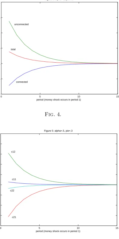
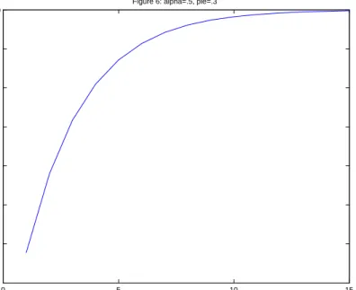
For thefirst experiment, setα =.5andπ =.3.The impulse responses are in Figures 4-6, where we show the ratios to the baseline case for employment and consumption in Figures 4 and 5 and the diﬀerence from the baseline case for the nominal interest rate in Figure 6. In Figure 4, note that employment rises in response to the money growth shock on unconnected islands and decreases on connected islands, with total employment increasing. In this experiment, the wealth eﬀects of the money injection dominate. Wealth increases for households on connected islands while it decreases for agents on unconnected islands, so that the connected-island households work less and

2_{This guarantees that cash-in-advance constraints are always binding in each of the three}

(23)

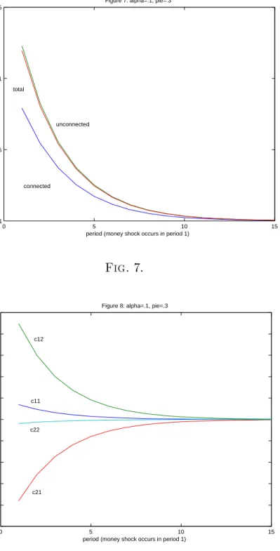
the unconnected island households work more. For all three employment quantities, the effects are quite small. However, this is not the case for consumption quantities, as in Figure 5 the money shock is shown to increase substantially the dispersion in consumption across agents. The increase in consumption is particularly large for consumers who live on a connected island and buy at a low price with a large quantity of money on an unconnected island. Similarly, the decrease in consumption is large for a consumer living on an unconnected island who must buy at a high price with a low quantity of money on a connected island. In Figure 6, the money shock produces a liquidity effect, with the increase in the money growth rate of 1% producing a decrease of about 30 basis points in the nominal interest rate on impact. Note also that the liquidity effect is persistent.

The decline in the nominal interest rate in response to a positive money shock occurs due to both a Fisher effect and an effect on the real interest rate. On connected islands, the price level will decline relative to the baseline case following the money shock, so deflation is anticipated and the Fisher effect acts to reduce the nominal interest rate. As well, households on connected islands expect their consumption to be falling over time following the money shock, and so the real interest rate will also be lower than if the money shock had not occurred.

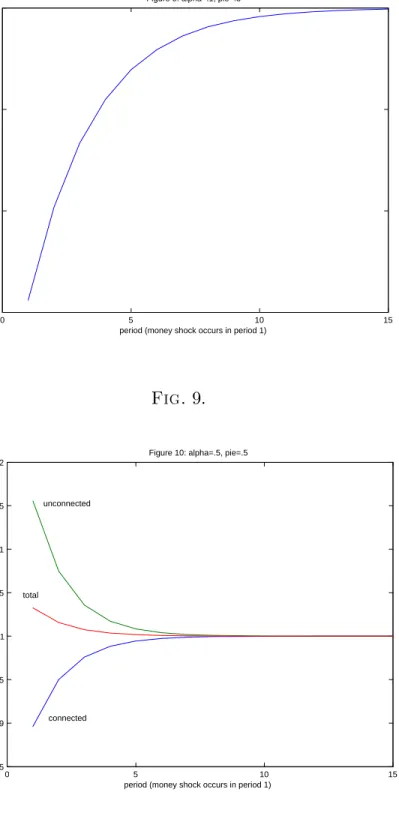
In the second experiment, we concentrate the money injection on fewer agents, set-tingα=.1andπ=.3.In this case, the results are shown in Figures 7-9, which should be compared to Figures 4-6. In Figure 4, note that the employment responses are somewhat larger, though still small, and that employment in all locations increases, in spite of the negative eﬀect of the increase in wealth on employment on connected islands. This is likely due to the fact that, withα small, the increase in consumption dispersion produced by the money shock is larger, as shown in Figure 8. As a result, the money shock produces more consumption uncertainty for all households, and this

(24)

0 5 10 15 0.999 0.9995 1 1.0005 1.001 1.0015 1.002

Figure 4: alpha=.5, pie=.3

period (money shock occurs in period 1)

la b o r s u p p ly connected unconnected total Fig. 4. 0 5 10 15 0.98 0.985 0.99 0.995 1 1.005 1.01 1.015 1.02 1.025

(25)

0 5 10 15 -0.35 -0.3 -0.25 -0.2 -0.15 -0.1 -0.05 0

n o m in a l in te re s t ra te i n % Fig. 6.

appears to be producing higher labor supply for everyone, in a manner much like a precautionary savings eﬀect. In Figure 9, note that the liquidity eﬀect is now larger than before, as each household on connected islands now receives a larger money in-jection given that we are holding constant the shock to the aggregate money growth rate.

In the third experiment, the money growth shock is less persistent, relative to the

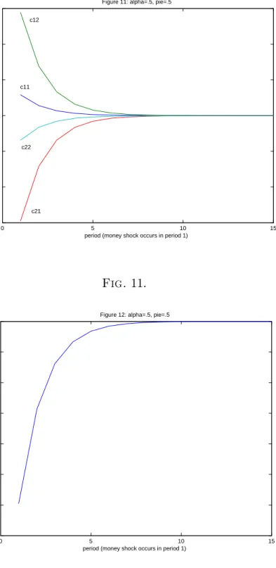
first experiment. The results are shown in Figures 10-12, which should be compared to Figures 4-6. Note in Figures 10 and 11 that the impact effects of the money shock on employment and consumption are similar, but the effects are less persistent as money is now diffused at a higher rate through the economy. Because of this more rapid diffusion, Figure 12 shows a larger liquidity effect on impact.

(26)

0 5 10 15 1

1.0005 1.001 1.0015

e m p lo y m e n t connected unconnected total Fig. 7. 0 5 10 15 0.95 0.96 0.97 0.98 0.99 1 1.01 1.02 1.03 1.04 1.05

(27)

0 5 10 15 -1.5

-1 -0.5 0

n o m in a l in te re s t ra te i n % Fig. 9. 0 5 10 15 0.9985 0.999 0.9995 1 1.0005 1.001 1.0015 1.002

e m p lo y m e n t connected unconnected total Fig. 10.

(28)

0 5 10 15 0.985 0.99 0.995 1 1.005 1.01 1.015

c o n s u m p ti o n c11 c12 c21 c22 Fig. 11. 0 5 10 15 -0.7 -0.6 -0.5 -0.4 -0.3 -0.2 -0.1 0

n o m in a l in te re s t ra te i n % Fig. 12.

(29)

CONCLUSION

We have constructed a model of heterogeneous households that captures some novel distributional eﬀects of monetary policy. In the model, some households find them-selves on the receiving end of a money injection by the central bank, and some do not. In general there will be price dispersion across markets generated by monetary policy, and as a result monetary policy can produce uninsured consumption risk. This consumption risk is important in determining optimal money growth rates and aﬀects the response of the economy to aggregate money shocks.

We showed that, for moderate levels of risk aversion, a constant money stock could be very close to optimal, and the welfare cost of a small inflation could be very large. In the experiments we conducted, money growth shocks have small effects on aggregate employment and large effects on the dispersion in consumption. There are potentially large and persistent liquidity effects, with the nominal interest rate declining in response to a positive money growth shock, even when money growth shocks are i.i.d.

REFERENCES

Alvarez, F. and Atkeson, A. 1997. “Money and Exchange Rates in the Grossman-Weiss-Rotemberg Model,”Journal of Monetary Economics 40, 619-40.

Alvarez, F., Atkeson, A., and Kehoe, P. 2002. “Money, Interest Rates, and Exchange Rates with Endogenously Segmented Markets,” Journal of Political Economy

110, 73-112.

Chiu, J. 2005. “Endogenously Segmented Asset Market in an Inventory Theoretic Model of Money Demand,” working paper, University of Western Ontario. Grossman, S. and Weiss, L. 1983. “A Transactions-Based Model of the Monetary

(30)

Transmission Mechanism,”American Economic Review 73, 871-880.

Head, A. and Shi, S. 2003. “A Fundamental Theory of Exchange Rates and Direct Currency Trades,”Journal of Monetary Economics 50, 1555-1592.

Lagos, R., and Wright, R. 2005. “A Unified Framework for Monetary Theory and Policy Analysis,” forthcoming, Journal of Political Economy.

Lucas, R. 1990. “Liquidity and Interest Rates,” Journal of Economic Theory 50, 237-264.

Rotemberg, J. 1984. “A Monetary Equilibrium Model with Transactions Costs,”

Journal of Political Economy 92, 40-58.

Shi, S. 1997. “A Divisible Model of Fiat Money,” Econometrica 65, 75-102.

Shi, S. 2004. “Liquidity, Interest Rates, and Output,” working paper, University of Toronto.

Williamson, S. 2005. “Search, Limited Participation, and Monetary Policy,” forth-coming,International Economic Review.