The Predictive Power of Alternative Volatility Forecasting Models over Multiple Horizons

i

The Predictive Power of Alternative Volatility Forecasting Models

over Multiple Horizons

Bikash Basnet (6030)

Supervisor Valeriy Zakamulin

This master’s thesis is carried out as a part of the education at the University of Agder and is therefore approved as a part of this education. However, this does not imply that the University answers for the

methods that are used or the conclusions that are drawn.

University of Agder, June 2016 School of Business and Law

2

Abstract

This thesis paper examines the forecast accuracy and explanatory power of volatility models over multiple forecast horizon for three asset classes. Forecast horizon ranging from 1 month up to 12 subsequent months are investigated using Naïve, EWMA, GARCH, EGARCH, GJR-GARCH and APARCH model for S&P 500, DJIA, CBOE(^TNX ), CBOE(^FVX), USD/CHF and GBP/CHF. MSE and Predictive Power (𝑃) are used to evaluate the forecast accuracy and predictive ability of the model over increasing horizon. Different distribution assumptions are also included with non-linear GARCH models in an attempt to improve forecast accuracy of the models. The in-sample estimation results revealed increased model fit for all assets considering the non-normal innovation but correspondingly didn’t always comply with out-of-sample forecast accuracy. Non-normal distribution provided best forecast accuracy at short forecast horizons for all asset classes except exchange rates. The result common to asset classes was that forecast accuracy and predictive power of the model are best at short horizon which gradually decreased with increasing forecast horizon. The predictive power suggested the longest forecastable horizon for Stock Indices, Interest Rates and Exchange rates are 4 months, 12 months and 2 months respectively. The results showed EGARCH model performed relatively well compared to other models and was able to increase the forecastable horizon. Further, it was concluded there is no best model for all asset classes over all horizons. The best model is largely dependent upon the type of asset and the horizon of interest.

3 Table of Contents

1. Introduction ... 4

2. Literature Review... 7

3. Data Analysis ... 13

3.1 Raw Data and Pretreatment ... 13

3.2 Plots of the Data ... 15

3.3 Shape Measures and Descriptive Statistics ... 18

3.4 Distribution... 20

3.5 Test for Stationarity ... 25

3.6 Test for ARCH effects... 26

4. Methodology ... 28

4.1 Forecasting Procedure ... 28

4.2 Forecasting Models ... 29

4.2.1 Naïve Forecasting Model ... 29

4.2.2 EWMA... 30 4.2.3 Basic Structure ... 31 4.2.4 ARCH ... 32 4.2.5 GARCH ... 33 4.2.6 EGARCH ... 34 4.2.7 GJR-GARCH ... 34 4.2.8 APARCH ... 35 4.3 Distribution Assumptions ... 36

4.3.1 The Normal Distribution (Gaussian) ... 36

4.3.2 The Student-t distribution ... 37

4.3.3 The Generalized Error Distribution ... 37

4.4 Forecast Evaluation ... 38 4.5 Predictive Power ... 39 5. Empirical Results ... 40 5.1 In-Sample Estimation ... 40 5.1.1 Stock Indices... 41 5.1.2 Interest Rates ... 42 5.1.3 Exchange Rates ... 43 5.2 Out-of-Sample Evaluation... 44 5.2.1 Stock Indices... 45 5.2.2 Interest Rates ... 48 5.2.3 Exchange rates ... 52 6. Discussion ... 55 7. Conclusion ... 58 Acknowledgements ... 60 References ... 61 Appendix 1: Results ... 66

4

1. Introduction

Volatility which we define as a measure for variation of the price of a financial instrument over time (Chen and Leonard, 1996) is not new to finance and economic literature. The discussion can be traced back to 1900 where Bachelier (1900) first used the term “coefficient of nervousness” or “coefficient of instability” to discuss the same thing.

Gerlach, Ramaswamy and Scatigna (2006) states financial volatility has varied considerably over time and has been generally high across the world since the early 1970s. Since then and especially after the stock market crash in 1987 volatility modeling and forecasting has been an indispensable topic of interest and research which has led to the introduction and practice of several volatility models over time. Figlewski (1997) states high volatility means high risk. In general, high volatility with its associated risk would be undesirable as it is seen as a symptom of market disruption, securities unfairly priced and malfunctioning of the market as the whole (Huq, Rehman, Rehman and Shahin, 2013). Thus, accurately modeling and forecasting volatility is necessitated which provides a key input to assess the investment risk associated and achieve a level of risk that market participants are willing to take.

Volatility and its predictability has been given due importance in several areas of finance. Markowitz (1952) on portfolio selection considered volatility as one of the fundamental variable in modern financial theory along with expected returns. Similarly, volatility has a key role in derivative pricing which can be noted from the option pricing model developed by Black and Scholes (1973) where among all other inputs, volatility is the only parameter which is unknown and needs to be forecasted from start date of the option till the expiry date in order to calculate option price. Other derivative products such as variance swaps and forward variance swaps offers direct exposure to volatility as an investment. This all makes volatility central to finance where accurate prediction are often sought by market participants to make more direct profits (Warren, 2012).

The enormous interest is reflected by the increasing number of researches and literatures regarding embedded dynamics of volatility on financial assets returns and its predictability. Many empirical

5 literature including that of Andersen and Bollerslev (1998) suggests volatility of assets return is time varying and predictable. Although “researchers agree that volatility is predictable in many asset markets, they differ on how this volatility predictability should be modeled” (Engle and Ng 1993; p.1749). Thus, over past few decades immense effort has been seen in literatures regarding modeling and forecasting time varying volatility (conditional heteroscedasticity). As a result, varied models have been developed and practiced to confirm its efficiency.

The first ever attempt was the introduction of autoregressive conditional heteroscedasticity (ARCH) model with normal innovation by Engle (1982) to model conditional heteroscedasticity in volatility. ARCH model performed particularly well when high ARCH order was selected but required many parameters to be estimated. Later, Bollerslev (1986) extended the ARCH model to Generalized Autoregressive Conditional Heteroscedasticity (GARCH) which emerged as the solution to the problem regarding high ARCH orders which required rather large number of parameters to catch the dynamic of the conditional variance. Brooks (1996), thus states GARCH model as infinite order ARCH model.

Financial assets exhibited some of the stylized statistical characteristics such as volatility clustering, heavy tails, leptokurtic distribution, absence of autocorrelations and leverage effect (Cont, 2001). Both ARCH and GARCH models successfully captured volatility clustering/persistence feature of the financial time series but omitted to look after the asymmetry of innovation to capture the leverage effect. To overcome this drawback different extension to the GARCH model have been proposed, some of which are deduced from pure theory and the others through simple trial and error suggestions (Tooma, 2000). The most popular extensions are Exponential GARCH (EGARCH) by Nelson (1991), Glosten-Jagannathan-Runkle GARCH (GJR-GARCH) by Glosten, Jagannathan and Runkel (1993) and Asymmetric Power ARCH (APARCH) by Ding, Granger and Engle (1993). Also the failure to capture the leptokurtic distribution of financial time series (i.e. fat tail property) by ARCH/GARCH models has led to the use of non-normal distributions within many non-linear extensions of the GARCH models including the ones discussed above (Thorlie, Song, Wang and Amin, 2014).

The primary purpose of this thesis is to investigate how the forecast accuracy and predictive ability of different models differs over long term horizons. Forecast horizons ranging from 1 month up to

6 12 months are investigated. Volatility predictability over forecast horizons are assessed through the use of seven different volatility models. The performance of these models out-of-sample forecast accuracy and predictive power against increasing horizon will be examined in order to fulfill the purpose. This thesis is expected to contribute to the existing knowledge base and literature in many ways. Firstly, unlike many papers, this thesis takes into consideration three asset classes; stock indices, interest rate and exchange rate data. Most of the existing researches are focused on pure assets market. The second contribution of this thesis is to analyze the performance of chosen models for subsequent months until 1 year. For many practical purposes, study on volatility forecast ability at longer horizons are interesting, but there are only few researches on the forecast accuracy of volatility models beyond the very short term (maximum 3 months). Thirdly, I use the method proposed by Blair, Poon, and Taylor (2001) to measure the explanatory power of the model which is also unique to existing literatures.

There are a lot of volatility forecasting models and it is not possible to cover all models. So, this thesis limits itself to use only seven models which are most used in empirical finance. However, it should be noted that there might exist other superior model for the selected assets return that could perform better against multiple horizons than that I have taken in consideration.

The rest of the thesis is structured as follows. The literature review is presented in Section 2 where I present some of the exiting researches that are focused on volatility predictability over multiple horizons. Section 3 includes presentation of the data which are further examined through descriptive statistics and different tests to reveal some of its properties. Section 4 will present the adopted econometric methodology where forecasting procedure, models, error distribution along with evaluation criterion are introduced. In Section 5, in-sample estimation and the forecast performance comparison results are presented and interpreted. The findings are compared and contrasted with existing relevant literatures in Section 6. Finally, in Section 7, main findings along with applied approach in this thesis is summarized and presented as conclusion.

7

2. Literature Review

Since the seminal paper of Engle (1982), a lot of empirical work has been carried out with non-linear ARCH-family model, especially in finance, in several practical situation. Yet, studying the predictability of different simple and ARCH-family models on multiple, especially long forecasting horizons have been considered only in limited papers.

Briefly, we find that, while different markets are different, throughout time financial market prices, prices of stock, bonds and exchange rates has shown striking changes in volatility. Thus, predicting volatility has been a growing concern and now is a proven fact that financial volatility are predictable as noted in Section 1. But the success of predicting volatility/forecast accuracy depends largely upon the defined horizon and the choice of horizon depends upon the application. One-day risk management approach is often used by risk managers for trading purposes (Smithson and Minton, 1996), while Falloon (1999) argues, approximately a year horizon is essential for investors and it may take as long up to ten years for pension fund.

Christoffersen and Diebold (2000), reviewing widespread empirical literatures, states academicians and researchers have often discussed on the importance of forecasting at varying horizon and argued upon the relevant horizon. But most notable was the emerging concern regarding forecasting at fairly long horizon which are relevant for several applications. Taking into consideration to this emerging concern in existing literature, they marked “ ….Interestingly, however, much less is known about volatility forecastability at longer horizons, and more generally, the pattern and speed of decay in volatility forecastability as we move from short to long horizons” (Pg;12). Decade later, still, we find very few literatures that studies volatility over longer horizons despite its emerging relevance in several applications. Existing empirical literatures have used multiple horizon for comparative study but are limited to very short horizon. In this thesis I use multiple horizon up to 1 year and compute the forecast accuracy for each subsequent month, using simple models and ARCH-family models taking into consideration the error distributions. Plus, rather than using a data from one specific sector as done in many literature, I chose three data from stock, interest rate and exchange rate market as it is obvious one

8 is concerned to know what works with one type of data will work correspondingly well with other type of data or not. Below are some relevant literatures.

Cao and Tsay (1992), using daily stock return derived a benchmark measure for the monthly volatility and compared the models for different forecasting horizon (1-30months). Evaluating means squared error (MSE) and mean absolute error (MAE), they concluded Threshold autoregressive (TAR) model outperforms ARMA (1,1), GARCH (1,1) and EGARCH (1,0) for large stocks while EGARCH (1,0) provides best long-horizon forecast for small stock. Viewing the post-sample forecast comparison of the paper it is also observable that over the forecasting horizon (1 to 30 months) forecast accuracy of the models gradually decreases.

Bluhm and Yu(2001) investigates over different horizon taking into account the practical application of volatility forecast in Value-at-Risk (VaR) (1 day and 10day) and option pricing (45 calendar days and 180 trading days). German DAX stock index and the DAX volatility index (VDAX) returns are used to model volatility using univariate time series approach and implied volatility approach. Mean absolute percent error (MAPE), boundary violation and LINEX are used as error measurement for different horizon. Not mentioning the clear winner they suggest stochastic volatility (SV) model and Implied Volatility should be used when option pricing and long horizon is of interest while the ARCH-type models works well when VaR is the objective. ARCH-type models predictive ability got worse when forecast horizon was extended. The other models used in this comparative study are historical mean model and EWMA model.

West and Cho (1994), using five bilateral weekly data for the dollar versus the currencies of France, Germany , United Kingdom, Canada and Japan, compared the forecasting performance using Homoscedastic, GARCH, Autoregressive and Nonparametric models for 1 week, 12 weeks and 24 weeks horizon. Models were evaluated using mean square prediction error (MSPE). Their study concluded that for a very short horizon of one week, GARCH type models (IGARCH especially) predictability was better than other models while it was difficult to find grounds to choose comparatively better model for longer horizons as models failed to perform well in the forecast efficiency test.

9 Li (2002) managed to apply the Autoregressive Fractionally Integrated Moving Average (ARFIMA) and Implied Volatility model for forecasting of currency volatility from 1 to 6 consecutive months. Coupled with the use of 5-minute data and daily returns with forward options on German deutschemark, the Japanese yen, and the British pound vs the US dollar, they found ARFIMA performed well on longer forecasting horizon while Implied Volatility suited well for short forecasting horizon.

Pong, Shackleton, Taylor and Xu (2002) compares the performance of the ARFIMA, ARMA (2, 1), GARCH (1, 1) model and option implied volatilities for forecast horizons ranging from 1 day to 3 months. Intraday rates are used to compute the realized volatility of the pound, mark and yen exchange rates against the dollar. Using MSE criterion, they find ARMA model performed better than implied volatilities for short forecast horizons while implied volatilities dominates when long forecast horizon is considered.

Heynen and Kat (1994) examined 7 stock indices and 5 exchange rates using SV, EGARCH (1, 1), GARCH (1, 1) and random walk (RW) model over non- overlapping 5,10,15,20,25,50,75 and 100 days horizon. Evaluating the model performance over horizons using median squared error (MedSE) they infer that volatility model forecasting performance depends on type of assets and SV outweighs other models however SV error is 10 times larger than GARCH models in exchange rate.

Figlewski (1997), puts together several line of research carried out over time to explore some of the major ways of forecasting volatility. Using the monthly and daily data the author provides insight on the problem of forecasting volatility over longer horizons. Historical volatility (HV) and GARCH (1, 1) model is used to model volatility while root mean square error (RMSE) is used to evaluate the forecast accuracy over multiple horizon (1, 3,6,12 and 24 months). GARCH (1, 1) model performed particularly well for S&P 500 index volatility at every horizon and RMSEs was increasing sharply over horizon reflecting decay of volatility predictability. However, for rest of the time series for bond and exchange rate HV has an edge over GARCH (1, 1) model.

Greeen and Figlewski (1999) forecasts volality for the S&P 500 stock index, 3-month LIBOR (short-term interest rate), 10-year T-Bond yield (long-term interest rate) and DM exchange rate

10 using daily data. HV and Exponential Smoothing (ES) are applied for asset classes over horizon form 1 to 12 month. Evaluating the models under RMSE, ES performed best for S&P 500 (1-3months) and 3-month LIBOR (all horizons). In contrast, HV provided the best prediction for bond yield, exchange rate and S&P 500 (12 months). When monthly data was applied, HV outperformed ES for all asset classes.

Ederington and Guan (2005), introducing a new models named absolute restricted least squares (ARLS) and GEN model compares its forecasting ability with historical standard deviation (HSD), EWMA, GARCH (1,1) , EGARCH (1,1) and AGARCH (1,1) model. Their analysis using RMSE and MAE in wide variety of market shows there is no clear choice between GARCH (1, 1) and EGARCH (1, 1). Both reflects better forecasting ability than HSD and EWMA. But when all models are considered, ARLS dominates every model in all forecasting horizons (10-120days). Ederington and Guan (2010), taking in consideration the Ederington and Guan (2005) model named ARLS compares among the GARCH (1, 1), GJR GARCH (1, 1), EGARCH (1, 1) and modified versions of these GARCH models. The modified GARCH models allowed for the parameters to vary with the forecasting horizon. Using RMSE and MAE across the forecasting horizon (10-80 days), they concluded that no one models predicts best in all markets at all forecast horizon. However, ARLS and modified EGARCH model provides better forecast over multiple horizons compared with other models across wide variety of market considered.

Apart from these empirical papers, there are few authors who have tried to answer the volatility predictability at multiple horizons using model free test procedures. The intuition behind model free test procedures was to study specifically on the pattern and speed of decay of predictability as we move form short horizon to longer horizon regardless of impact of volatility models on multiple horizons. Thus, to evaluate predictability of volatility per se, Christoffersen and Diebold (1998) developed a model free test procedure where they evaluate data from stock, bond and foreign exchange market. Their results reflected that depending on the asset classes, over increasing horizon predictability decays quickly and becomes largely unpredictable. They found that volatility is more forecastable in bond market compared to stock and exchange rate market. Later, Raunig (2006) introduced a new model free test procedure which was more powerful in monte-carlo experiment to evaluate the predictability of DAX index volatility. Using this new test, Raunig

11 (2006) found volatility decayed rather slowly and DAX index was predictable to 40 trading days ahead which was predictable to only about 15 trading days before. Raunig (2008) used the simulation version of same test he developed in Raunig (2006) to study the predictability of exchange rate volatility where he finds predictability declines rather quickly and exchange rate volatility is hard to predict for more than 1 month ahead.

For the financial time series volatility clustering, leptokurtosis and leverage effect are common phenomenon (Mandelbrot, 1963 and Black, 1976). GARCH models in its standard form assumes that the conditional distribution of asset returns is Gaussian. However, when high frequency time series data are used GARCH models do not fully embrace the thick tail property (Curto et al., 2009). To overcome this drawback different non-normal alternative distributions has been proposed. Bollerslev (1987) used and recommends using Student-t distribution. Nelson (1991) suggests using the generalized error distribution (GED). This thesis limits itself to use only three distributional model of innovation; Normal, Student-t and GED taking in consideration the finding of Wilhelmsson (2006) where allowing for skewness didn’t lead to any improvement over normal distribution. Below I present two researches which considers both multiple horizon and distribution assumptions. It is to be noted that horizon considered is no more than a month as none of the paper were found to have longer horizon which also considered distribution assumption. Marcucci (2005) explored GARCH (1, 1), EGARCH (1, 1), GJR-GARCH (1, 1) and Markov Regime-Switching GARCH (MRS-GARCH) models taking into consideration normal, student-t and GED distribution. Using the S&P 100 daily closing price the author aims to compare between the models considering varying horizon (1 day, 1 week, 2 week and 1month). The empirical analysis reveals that over a longer horizon, standard asymmetric GARCH model with non-normal innovation performed well while MRS-GARCH outweigh other models at shorter horizons. Wilhelmsson (2006) employed intra-daily returns from S&P 500 index future to investigate the forecasting ability of the GARCH (1, 1) model when estimated with nine different error distribution. The MAE and HMAE (Heteroscedasticity adjusted MAE) reveals GARCH (1, 1) model estimated with student-t is the best performing model for 1 and 5 days forecast. For the 20 days forecast, this model has the lowest `MAE but is close second on HMAE loss function. This result partially agrees with Hamilton and Samuel (1994), who showed GARCH (1, 1) model with

12 t-distribution to perform best when logarithm loss criteria is used. The out of sample analysis in Wilhelmsson (2006) further shows allowing for kurtosis/leptokurtic error distribution improves forecasts while allowing for skewness doesn’t lead to any improvement over normal distribution. On the basis of empirical papers reviewed it can be inferred that there is no generally accepted model or method for all assets. The performance of the volatility models seems to be dependent upon researcher’s preferences in terms of assets under study, sampling period, data frequency, forecast methods, evaluation criteria, forecast horizon etc. In addition, over the increasing forecast horizon the gradual decrease in forecasting ability of the models are also dictated. The non-normal distribution is attributed to improve the forecast accuracy over normal distribution. When considering the three asset classes in relevant papers the common finding was that volatility is more forecastable in bond market compared to stock market and exchange rate market. The predictability of exchange rates was found to decay rather quick which usually becomes hard to predict after 1 month.

Further, Implied volatility as an alternative source of volatility forecast are shown to be powerful in many studies discussed above but Ederington and Guan (2010), states time series models still remain a major source of volatility forecasting as implied volatility as an alternative source must reflect much information including time series information. In addition, they argue except for limited set of assets and for specific time horizons, implied volatility cannot be simultaneously be used to price the derivative from whose price they are calculated. Thus, in this thesis I use time series models to forecast volatility which are introduced in Section 4.

13

3. Data Analysis

3.1 Raw Data and Pretreatment

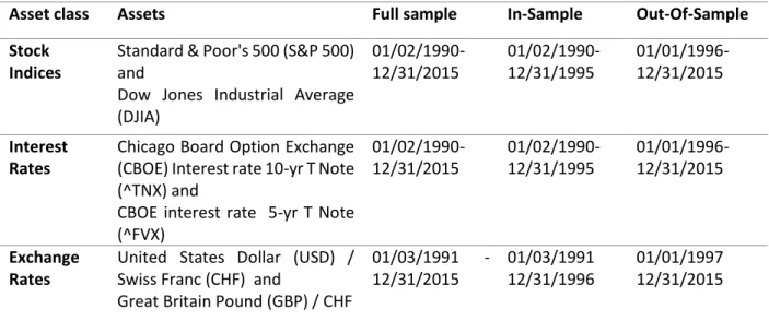
Two sets of data each for stock index, interest rate and exchange rate are used in this thesis for empirical study. In particular, the data set to be investigated consist of following assets

Table 1: Selected assets for each asset class to be used in forecasting application and the first and last date of the full sample, in-sample and out-of-sample period.

Under Stock Indices, S&P 500 and DJIA are chosen for analysis purpose. The S&P 500 is a market value weighted index of 500 most extensively traded stocks in United States (U.S). This index is regarded as a better representation of U.S. marketplace as it contains about 70% of the total value of overall U.S. stock market. DJIA, on the other hand is a price weighted index of 30 most largest and influential companies of U.S and represents about quarter of the total value of overall U.S. stock market (www.investopedia.com).

For interest rates, CBOE (^TNX) and CBOE (^FVX) are chosen. Both of them are closely watched long term and medium term U.S. Treasury securities which can represent the general economic condition, monetary and fiscal policies, value of U.S. dollar etc. CBOE (^TNX) and CBOE (^FVX) are based on yield-to-maturity of the most recently auctioned 10-year and 5-year Treasury notes respectively (www.cboe.com).

Asset class Assets Full sample In-Sample Out-Of-Sample Stock

Indices

Standard & Poor's 500 (S&P 500) and

Dow Jones Industrial Average (DJIA) 01/02/1990-12/31/2015 01/02/1990- 12/31/1995 01/01/1996-12/31/2015 Interest Rates

Chicago Board Option Exchange (CBOE) Interest rate 10-yr T Note (^TNX) and

CBOE interest rate 5-yr T Note (^FVX) 01/02/1990- 12/31/2015 01/02/1990- 12/31/1995 01/01/1996- 12/31/2015 Exchange Rates

United States Dollar (USD) / Swiss Franc (CHF) and

Great Britain Pound (GBP) / CHF

01/03/1991 -12/31/2015 01/03/1991 12/31/1996 01/01/1997 12/31/2015

14 For exchange rates, CHF being the common currency, USD against CHF and GBP against CHF are chosen.

Two sets of representative assets in each asset class are used as it is comprehended that different assets although being the same kind doesn’t always seem to move in tandem. So, by analyzing the assets from the same asset class it would be easier to make deductions on their similarities and differences. Further, different asset classes are taken in consideration to see if what works with one type of asset class will work correspondingly well with other type of asset class or not. The data sets are built considering the daily closing price of each assets for the given time period. The daily historical closing prices for stock indices and interest rates are gathered from Yahoo Finance (www.finance.yahoo.com) while for exchange rates the data are gathered from Oanda (www.oanda.com). The full sample consist of twenty five years of data for stock indices and interest rates, and twenty four years of data for exchange rates due to the unavailability of data from 1990. The full sample period is broken into in-sample period of five years and remaining period as out-of-sample forecasting period for all assets.

Daily closing price of assets are used to calculate the daily returns for the whole sample. The return series so obtained are often preferred over raw price series when the interest of study is related to financial time series. Campbell, Lo and MacKinlay (1997) states return series are easier to handle and is a more complete, scale free summary of particular investment opportunity. Assuming 𝑝_𝑡, as the daily closing prices for the given assets, daily logarithm return, 𝑟_𝑡, for the time series in this thesis is calculated as:

𝑟_𝑡 = 𝑙𝑜𝑔(𝑝_𝑡) − 𝑙𝑜𝑔(𝑝𝑡−1) = 𝑙𝑜𝑔 ( 𝑝𝑡

𝑝𝑡−1) (1)

On the basis of so obtained daily return time series for representative assets relevant graphical and numerical descriptive statistics are discussed below to investigate the distribution and dependence properties of daily assets returns. Exploratory data analysis of such kind will assist to see if the time series are well suited to apply ARCH-family models with different error distributions for forecasting.

15

3.2 Plots of the Data

Time plots are the most convinient way to quickly visualize the time series data with time index set to x-axis and time series data set to y-axis. Below I plot daily closing prices and retruns for all asset classes and jot down few phenomena that are explicit from the figures.

Figure 1: End-of-day closing prices for Stock Indices

16 Figure 3: End-of-day closing prices for Exchange Rates

The given Figure 1, 2 and 3 represents the daily closing prices for different asset classes. Visualizing the time plots, the movement of price can be seen for all assets from 1990 to 2015. The movement shows upward trend for stock indices while for interest rates and exchange rates downward trend can be visualized. Overall the price series appears to be non-stationary and exhibit random walk like behavior. For all assets, it can be seen there is no tendency to return around time independent mean.

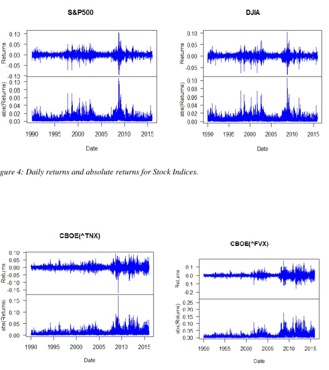
However, the time plots for return series displays that the returns oscillates around the mean value which is depicted in Figure 4, 5 and 6.

17 Figure 4: Daily returns and absolute returns for Stock Indices.

18 Figure 6: Daily returns and absolute returns for Exchange Rates.

Different phase (periods) of volatility for assets return are evident from Figure 4, 5 and 6 for all assets where low periods of volatility is likely to be followed by periods of low volatility and high periods of volatility is likely to be followed by period of high volatility. This feature that is often pronounced as stylized fact in financial time series data is known as volatility clustering as noted by Mandelbrot (1963), and is a necessary condition for the application of ARCH model. Zivot (2015) corresponds this type of behavior to conclude volatility of assets return exhibit some time dependence.

3.3 Shape Measures and Descriptive Statistics

The shape measures for the return distribution reflects the measure for center, spread, asymmetry and tail thickness. The corresponding shape measure of return distribution of data sample are represented by the sample summary statistics in the Table 2.

Mean, 𝜇̂𝑥, is the measure of center of histogram.The spread of the data from the calculated mean

is measured by sample variance, 𝜎̂_𝑥2_{, and sample standard deviation,𝜎̂}

𝑥. Sample skewness, 𝑆𝑘𝑒𝑤̂ 𝑥,

and sample kurtosis, 𝑘𝑢𝑟𝑡̂_𝑥, is a measure of asymmetry and tail thickness of the histogram respectively (Zivot, 2015). The formula for calculating the discussed sample statistics of return are:

19 𝜇̂_𝑥= 𝑥̅ = 1 𝑇∑ 𝑥𝑡 𝑇 𝑡=1 (2) 𝜎̂𝑥2 = 1 𝑇−1∑ (𝑥𝑡− 𝑥̅) 2 𝑇 𝑡=1 (3) 𝜎̂_𝑥= √𝜎̂_𝑥2 ₍₄₎ 𝑆𝑘𝑒𝑤̂ =𝑥 1 𝑇−1∑ (𝑥𝑡−𝑥̅) 3 𝑇 𝑡=1 𝜎 ̂𝑥3 (5) 𝐾𝑢𝑟𝑡̂ = 1 𝑇−1∑ (𝑥𝑡−𝑥̅) 4 𝑇 𝑡=1 𝜎 ̂𝑥4 (6) Where,

T is the sample size and

𝑥_𝑡 is the observation at time period t.

Asset Class Stock Indices Interest Rates Exchange Rates Assets S&P500 DJIA CBOE(^TNX) CBOE(^FVX) USD/CHF GBP/CHF No of observation 6552 6540 6524 6524 7118 8953 Minimum -0.0947 -0.080 -0.1702 -0.2641 -0.1761 -0.1796 Median 0.0005 0.0005 -0.0004 0.0000 0.0000 0.0000 Arithmetic Mean 0.0003 0.0003 -0.0002 -0.0002 0.0000 -0.0001 Geometric Mean 0.0002 0.0002 -0.0003 -0.0005 -0.0001 -0.0001 Maximum 0.1096 0.1051 0.0922 0.1772 0.0924 0.0829 Variance 0.0001 0.0001 0.0003 0.0006 0.0000 0.0000 Std 0.0114 0.0109 0.0160 0.0238 0.0065 0.0052 Skewness -0.2399 -0.1353 0.0190 0.0172 -2.4785 -4.4469 Excess Kurtosis 8.65 8.2244 5.5457 7.7424 87.7252 184.8697

Table 2: Summary statistics of return

The number of observation for the data sets varies due to the different number of trading days. For the exchange rates the sample date starts one years after as depicted in Table 1.

20 Mean and median for the return series are very close to 0. Standard deviation for exchange rates are quite low compared to stock indices and interest rates. The percent difference between the maximum and minimum return shows the price variability. CBOE (^FVX) has the highest price variability with 44.13 percent difference which corresponds to the higher value of standard deviation compared among all other assets.

The sample skewness for interest rates are 0.0190 and 0.0172 for CBOE (^TNX) and CBOE (^FVX) reflecting approximate symmetry. The negative skewness values of stock indices and exchange rates reflects that the distributions are skewed left. The skewedness for exchange rates is significant compared to rest of the asset classes. The excess kurtosis (kurtosis - 3) indicate that the distribution have much fatter tails. Brooks and Hinich (1998) notes that the exchange rates are highly leptokurtic which is in line with our excess kurtosis values of 87.72 and 184.87 for USD/CHF and GBP/CHF respectively. The values so obtained from skewness and kurtosis proposes that the distribution of returns may be not normally distributed which we will confirm below using various means.

3.4 Distribution

Distribution of returns rather than prices are focused in this study as prices tends to be non-stationary. (Zivot, 2015) argues for sample descriptive statistics to be meaningful only for covariance stationary and ergodic time series.

The distribution is of particular interest in this thesis, thus, we explore it through various graphical and numerical presentations. Firstly, we review the histograms which graphically summarizes the distribution of the time series data.

21 Figure 7: Histogram for Stock Indices

22 Figure 9: Histogram for Exchange Rates

The figures depicted above provides the graphical representation of data with normal curve superimposed. The superimposed normal curve is given by the bell shaped blue line in all figures. The histograms in Figure 7,8 and 9 instantly gives us the idea that the distribution of data are tall and skinny (peaked) relative to standard bell curve. This is a property knowns as leptokurtic/fat tail distribution and true for all financial time series data. This leptokurtic property is parallel for the positive kurtosis generated for all assets.

Thus, the histogram does provide us with the visual measure of shape to infer whether the data are normally distributed or not but it is not considered effective way of looking at systematic departure from normality. However, a normal Q-Q plot quite effectively shows the level of normality.

23 Figure 10: Normal Q-Q plots of Stock Indices.

24 Figure 12: Normal Q-Q plots of Exchange Rates.

In Figure 10, 11 and 12 the blue dots represents the actual data. These actual data are placed against the horizontal black line (standard normal distribution). If the dots adheres to the horizontal line, the distribution of data is considered to be normal while the deviation from horizontal line represents non-normality. Normal Q-Q plots presents the plots curving away quickly from the line at each end in opposite directions due to the presence of leptokurtic property which was also evident in histogram with peaked distribution.

In addition to these visual representations for normality, calculation in numeric terms is considered equally important since the look at the patterns through plots and bars are sometimes inconclusive. So, Jarque-Bera (JB) test is carried out to test if assets returns follow normal probability distribution. The JB test statistics is calculated as:

𝐽𝐵 = 𝑛 [𝑆

2

6 +

(𝐾 − 3)2

25 Where,

𝑛 - Sample size 𝑆 - Skewness and 𝐾- Kurtosis

The test statics of JB test is chi-squared distributed with 2 degrees of freedom under the null hypothesis. The null hypothesis for JB test is a joint hypothesis of skewness and kurtosis being 0 and 3 respectively. Rejection of null hypothesis at 5% significance level suggests that the distribution of data is not normal (Gujarati, 2003).

Asset Class Stock Indices Interest Rates Exchange Rates Assets S&P500 DJIA CBOE(^TNX) CBOE(^FVX) USD/CHF GBP/CHF Test Statistic 20492 18452 8361 16295 2289708 1277880 P Value 2.2e-16 2.2e-16 2.2e-16 2.2e-16 2.2e-16 2.2e-16

Table 3: Jarque-Bera Test statistics for Stock Indices, Interest Rates and Exchange Rates.

For all the assets, JB test statistics is quite high and P value is less than the critical value of 0.05. So, the null hypothesis is rejected to conclude that the series is clearly not normally distributed confirming to what is shown by histograms and Q-Q normal plot.

3.5 Test for Stationarity

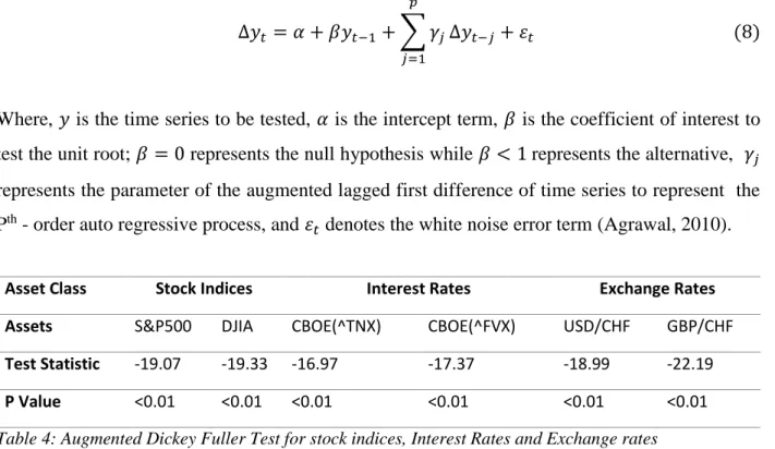
A time series is assumed to be stationary if its mean, variance and autocovariances for each given lag is constant over time (Brooks, 2008). A unit root test is applied to examine the stationarity or non-stationarity of the time series. A simple and obvious method would be to examine autocorrelation function of the return series but Brooks (2008) criticizes this method being misleading and not suitable to conclude whether a series is characterized by unit root or not. Rather he proposes to use augmented dickey- fuller test (ADF) test. Under ADF test, null hypothesis that the time series is non-stationary is compared against the alternative hypothesis of stationarity. The ADF test specification is constructed as:

26 ∆𝑦𝑡= 𝛼 + 𝛽𝑦𝑡−1+ ∑ 𝛾𝑗

𝑝

𝑗=1

∆𝑦𝑡−𝑗+ 𝜀𝑡 (8)

Where, 𝑦 is the time series to be tested, 𝛼 is the intercept term, 𝛽 is the coefficient of interest to test the unit root; 𝛽 = 0 represents the null hypothesis while 𝛽 < 1 represents the alternative, 𝛾𝑗

represents the parameter of the augmented lagged first difference of time series to represent the Pth - order auto regressive process, and 𝜀_𝑡 denotes the white noise error term (Agrawal, 2010).

Asset Class Stock Indices Interest Rates Exchange Rates Assets S&P500 DJIA CBOE(^TNX) CBOE(^FVX) USD/CHF GBP/CHF Test Statistic -19.07 -19.33 -16.97 -17.37 -18.99 -22.19 P Value <0.01 <0.01 <0.01 <0.01 <0.01 <0.01

Table 4: Augmented Dickey Fuller Test for stock indices, Interest Rates and Exchange rates

Table 4 shows ADF test statistics for the assets return. The negative values for test statistics and P-value less than 0.01 suggests null hypothesis is rejected at 1% significance level, inferring that all the return series are stationary.

3.6 Test for ARCH effects

Zivot and Wang (2006) recommends to test for the presence of ARCH effect in the residuals before estimating a full ARCH model for the return series. Among many methods available, Lagrange Multiplier (LM) test (ENGLE, 1982) is chosen which has been widely used to test the presence of conditional heteroscedasticity and ARCH effects.

Given, conditional variance, 𝜎_𝑡2_{, ARCH model which is represented by Equation 19 (see Section}

4), the AR (p) process for the squared residuals is constructed as:

𝜀_𝑡2 = 𝛼0+ 𝛼1𝜀𝑡−12 + ⋯ + 𝛼𝑝𝜀𝑡−𝑝2 + 𝜇𝑡 (9)

27 ARCH-LM test statistics is calculated as:

𝐿𝑀 = 𝑇. 𝑅2~𝑋2(𝑝) (10)

Where, T represent the sample size and 𝑅2 is computed from the regression of Equation 9 and p denotes the number of lags placed on the model. Under ARCH-LM test, null hypothesis suggests there is no ARCH effect. That is 𝛼1 = 𝛼2 = ⋯ = 𝛼𝑝 = 0 (Zivot and Wang, 2006)

Table 5: ARCH-LM test for Stock Indices, Interest Rates and Exchange Rates

ARCH-LM test presented in the Table 5 suggest that all assets exhibit ARCH effect as the P values are essentially zero. The null hypothesis is rejected even at 1% significance level. Hsieh (1989) argues that return series that shows the presence of ARCH effect implies that nonlinearities must enter through the variance of the processes. Such behavior can be essentially captured by considering ARCH-family structures in the model. Lee and king (1993) argues that the test can also be used as a general specification for GARCH effect even though it is derived from the ARCH model.

Thus, the presence of the established stylized facts and ARCH effect gives credence to the use of ARCH-family models for estimation with different error distribution.

Asset Class

Stock Indices Interest Rates Exchange Rates Assets S&P500 DJIA CBOE(^TNX) CBOE(^FVX) USD/CHF GBP/CHF Test

Statistic

1420 1280 583.9 606.8 136.3 179.8

28

4. Methodology

4.1 Forecasting Procedure

Time series forecasting is essentially an attempt to predict the future values of series given its historical values. Brooks (2008) discusses two methods to generate a series of forecasted values for the given step size. The first method is using a recursive forecasting model that exercises expanding window where initial estimation date is fixed and additional observations are consecutively added depending on the step size to the estimation period. In contrast, the second method is using a rolling window where fixed in-sample length coupled with defined step size is used. Start date and end date is set to successively increase by assigned value of observations/steps. In this thesis forecasting procedure uses the rolling window which closely follows to earlier empirical studies (see Brooks (1998) or Akgiray (1989)).

Under rolling window, return series is divided into two parts where the volatility in out-of- sample period (testing sample) is forecasted using the in-sample period (estimation sample). The sum of testing sample and estimation sample presents the total sample size. In this thesis, assuming 21 trading days in a month we have in average 6300 daily observations for the return series. In-sample period of 5 years is used which gives us 1260 observations to estimate the parameter of the model and create the first forecast of volatility for assigned step size/n-days. For successive forecast, the estimation sample is rolled forward by dropping the initial assigned step size/n-days observations and adding in the new observations. This process of out-of-sampling forecasting allows for the modification of model parameter over time and until the conditional variance for the forecast are sought.

This mechanism is used for all the return series. Once we get the conditional variance through the given scheme, forecast of the volatility for time period t is calculated which is given by:

𝜎̂𝑡 = √∑ 𝜎̂𝑖2 𝑁

𝑖=1

29 Where,

𝜎̂𝑡 is the standard deviation for time period t

𝜎̂_𝑖2 is the sum of squared daily variance and 𝑁 is the number of days for time period t

To investigate the performance of various models once volatilities (𝜎̂𝑡 ) are forecasted, it has to be

compared against actual volatilities. But actual volatility is unobservable. So, it is obvious to rely on proxy for realized volatility. Andersen and Bollerslev (1998) argues for the need of intraday return to correctly estimate the actual volatility. But since the intraday returns are not readily available the common accepted method is to use the squared daily returns as the unbiased estimator of realized volatility. Awartani and Corradi (2005) suggests using (𝑟_𝑖 − 𝑟̅)2 as a proxy for latent volatility when the true underlying volatility process is not observable. So, the proxy used for realized volatility at time period t is calculated using the given formula.

𝜎_𝑡 = √∑(𝑟_𝑖− 𝑟̅)2 𝑁 𝑖=1 = √∑ 𝑟_𝑖2 𝑁 𝑖=1 (12)

Where, 𝑟_𝑖 is the daily return and

𝑁 is the number of trading days for a chosen period.

4.2 Forecasting Models

4.2.1 Naïve Forecasting Model

This is one of the most straightforward and simplest historical price model to forecast volatility of time series data. This model gives importance to the most current observation assuming that all other past observations doesn’t provide any information for the future. That is, all the forecast are simply set to be the value of the last observation (Hyndman and Athanasopoulos, 2013). In other

30 words, the optimal forecast for the next period volatility (𝜎̂t+1) is simply the realized volatility of current period i.e. (σt). This can be expressed as:

𝜎̂_𝑡+1= 𝜎_𝑡 (13)

This method of forecasting is considered to work quite well for many economical and financial time series and is considered to be a convenient benchmark as the values of 𝜎_𝑡 are readily available. However, it is argued that the model cannot be used in long run forecasting and is criticized for being too persistent (Zakamulin, 2014). This model is used as a benchmark model in this thesis. 4.2.2 EWMA

Essentially exponentially weighted moving average (EWMA) model is a simple extension to historical average volatility measure. EWMA specifications allow the most recent observation to carry more weight to have stronger influence on volatility forecasting while the weights on old observations will decline exponentially with time (Brooks, 2008). EWMA estimates of the volatility can be expressed as:

σ ̂_𝑡 2 = (1 − λ) ∑ λ𝑗 𝑛 𝑘=0 (r_t−j− r) (14) Where,

σ̂_𝑡 2 is the estimate of the variance.

r is the average return of observations and λ is the decay factor

The forecasting from EWMA over different horizons is the most recent weighted average estimate and λ controls the estimation of daily volatility. It is important to note that most of the academic studies set r to zero (Brooks, 2008). Most often the value of λ lies in between 0.94 to 0.97 (0.96 in this thesis) aiming to maximize the forecast accuracy. The model deems to be unsuitable for long run forecasting (Zakamulin, 2014).

31 4.2.3 Basic Structure

Jondeau, Poon and Rockinger (2007) states as high frequency time series data are not readily available using lower frequency data such as daily returns are most often practiced by academicians and researchers. In such a condition of using daily data they propose for the use of ARCH/GARCH models which intuitively describes time variation in conditional volatility. The use of ARCH/GARCH models reflect to some extent the fat tails phenomena present in the return series. However, to capture the leverage effect present in return series effectively different asymmetric GARCH models have been developed and practiced.

The basic structure of volatility model is presented as:

𝑥_𝑡 = 𝜇_𝑡(𝜃) + 𝜀_𝑡 (15) 𝜀_𝑡 = 𝜎_𝑡(𝜃)𝑍_𝑡 (16) Where, 𝜇_𝑡(𝜃) = 𝐸[𝑥_𝑡 ∣ 𝐹_𝑡−1] 𝜎_𝑡2_{(𝜃) = 𝐸[(𝑥} 𝑡− 𝜇𝑡(𝜃)) 2 ǀ 𝐹_𝑡−1

Where in Equation 1 return xt is decomposed into conditional mean µ and a residual term or past innovation ɛt. Conditional mean (µt (Ɵ)) may consider ARMA (p, q) process or consist of the seasonality features. Ft is the information set available at the time period t and Ɵ is the vector of unknown parameter. Zt in Equation 16 is assumed to follow some distribution with mean 0 and variance 1.

ARCH-family and Stochastic volatility models are two variety of volatility models that describes the evolution of 𝝈2 _{(Ɵ). ARCH-family model describes volatility as an exact function of a given} set of variable while stochastic model describes volatility as a stochastic function. (Jondeau et al, 2007). In this thesis I use ARCH-family model to describe the dynamics of volatility.

32 4.2.4 ARCH

First introduced by Engle (1982), Autoregressive conditional heteroscedasticity (ARCH) model addresses and models the conditional heteroscedasticity in volatility. The ARCH process leaving the unconditional variance constant allows the conditional variance to vary over time as a function of past innovation (Bollerslev, 1986).

A univariate ARCH models basically consist of conditional mean equation and conditional variance equation to model the first and second moment of return respectively (Brooks, 2008). Thus, the structure of ARCH (p) volatility model is presented by mean equation and conditional variance equation which is stated below in Equation 17 and Equation 19 respectively.

𝑥_𝑡 = 𝜇 + 𝜀_𝑡 (17) 𝜀_𝑡 = 𝜎_𝑡𝑍_𝑡 (18) 𝜎_𝑡2 = 𝜔 + 𝛼1𝜀(𝑡−1)2 + ⋯ + 𝛼𝑝𝜀𝑡−𝑝2 = 𝜔 + ∑ 𝛼𝑖𝜀𝑡−𝑖2 𝑝 𝑖=1 (19)

Where, ⍵, 𝛼 and 𝑝 denotes intercept, arch parameters and number of lags respectively. The constraints of parameters 𝜔 ≥ 0 and 𝛼_𝑖 ≥ 0 (i = 1… p) ensures that the conditional variance 𝜎2 is positive and the model is well defined. 𝜀_𝑡2, is the square error obtained from the mean equation (Jondeau et.al, 2007).

Despite the ARCH model ability to model volatility clustering, excess kurtosis and mean reverting characteristics this model has been severely criticized for not considering the asymmetric effect and requiring large value of 𝑝 to successfully capture all of the dependence in the conditional variance. Similarly, non-negativity constraints might be violated as one or more of the parameters may have negative estimated values with increasing parameters in conditional variance equation (Brooks, 2008). Due to these problems ARCH model has been hardly been used over last decade.

33 This model will not be used in this thesis but is defined here as this model provided a framework for the analysis and development of other volatility models which are discussed below.

4.2.5 GARCH

Bollerslev (1986) proposed extension to the ARCH model which is empirically considered more parsimonious, as ARCH model required large number of p to successfully model the large persistence of volatility.

Brooks (2008) states under GARCH model the conditional variance is modeled as an ARMA process which allows the conditional variance to be dependent on its previous own lags. This means that the conditional variance in GARCH model is a weighted average of past squared residuals and these residuals are assumed to decline geometrically. The Equation 17 along with the conditional variance equation given in Equation 20 represents the basic GARCH (p, q) model.

𝜎_𝑡 2 _{= 𝜔 + 𝑖 ∑ 𝛼} 𝑖 𝑝 𝑖=0 𝜀_𝑡−𝑖2 + ∑ 𝛽_𝑗𝜎_𝑡−𝑗2 𝑞 𝑗=0 (20)

Under GARCH specification, conditional variance changes over time while unconditional variance of 𝜀_𝑡 is finite and is expressed as:

𝜎̅2 = 𝑣𝑎𝑟(𝜀_𝑡) = 𝜔

1 − (∑𝑝_𝑖=1𝛼_𝑖 + ∑𝑞_𝑗=1𝛽_𝑗) (21)

Under the equations above, the constraints of parameters 𝜔 ≥ 0 , 𝛼_𝑖 ≥ 0 ( i = 1,…..,p) , 𝛽j ≥ 0 (j=1,…..,q) ensures that the conditional variance σ2_{t is non-negative and ∑ 𝛼}

𝑖 + ∑𝑞𝑗=1𝛽𝑗 𝑝

𝑖=1 < 1

ensures that the process 𝜀_𝑡 is covariance stationary. If q =0, the model reduces to ARCH (p) model (Jondeau et.al, 2007). .

Along with the beauty of requiring far less parameters, Brooks (2008) considers GARCH model to be parsimonious as it avoids overfitting of data and the probability that non-negativity constraints will be breached is lower. However, Greeen and Figlewski (1999) argues against

34 GARCH model as it required large data set for reliable estimation and its potential gain from the approach are quickly moderated when estimates must be made over longer horizons. GARCH model are further criticized for its inabalility to model assymetric effect

4.2.6 EGARCH

EGARCH model as an extension to GARCH model was proposed by Nelson (1991) to overcome the drawbacks inherent in symmetric GARCH model. Basically it addressed two issues; the first regarding the need that parameters 𝛼 and 𝛽 have to be constrained to ensure non-negativity in conditional variance, 𝜎_𝑡2, and the second regarding the ability to incorporate asymmetric response of volatility to positive and negative shocks (Jondeau et.al., 2007). The log of conditional variance equation below represents the basic EGARCH (p, q) model.

log(𝜎_𝑡2) = 𝜔 + ∑ 𝛼𝑖𝑔(𝑧𝑡−𝑖) + ∑ 𝛽𝑗log(𝜎𝑡−𝑗2 ) 𝑞 𝑗=1 𝑝 𝑖=1 (22) Where, 𝑧𝑡 = 𝜀𝑡

ℎ𝑡 is the normalized residual

𝑔(𝑧𝑡) = [𝛾(|zt| − E[|zt|]) + 𝜓𝑧𝑡] ; represents 𝑔(𝑧𝑡) as the function of both sign (𝜓𝑧𝑡 ) and the

magnitude ([𝛾(|zt| − E[|zt|]) of 𝑧𝑡. The value of E[|zt|] changes under different assumed

density distribution.

Under EGARCH specification, the conditional volatility is always positive, so, the parameters are not restricted to be non-negative. But ∑𝑞_𝑗=1𝛽 < 1 is necessary condition for the process to be covariance stationary (Jondeau et.al. 2007).

4.2.7 GJR-GARCH

Glosten et.al (1993) proposed an alternative method to model the asymmetric response of volatility to positive and negative shocks known as GJR-GARCH model. Including an additional term they

35 simply extended the GARCH model to capture the possible asymmetries. With 𝜀𝑡 assumed to be

same structure as before (Equation 18), the conditional variance for GJR-GARCH (p, q) is represented by:

𝜎𝑡2 = 𝜔 + ∑𝑝𝑖−1[𝛼𝑖𝜀𝑡−𝑖2 + 𝛾𝑖𝐼𝑡−𝑖𝜀𝑡−𝑖2 ] + ∑𝑞𝑗=1𝛽𝑗𝜎𝑡−𝑗2 (23)

Where, the indicator 𝐼_𝑡−𝑖 takes the value of one if 𝜀_𝑡−1< 0 which is otherwise 0. The parameter 𝛾𝑖 is the leverage term which is usually impacted by positive shocks while negative shocks

impacts 𝛼_𝑖. Depending on the positive or negative value of 𝜀_𝑡 the impact of 𝜀_𝑖2 on conditional variance 𝜎_𝑡2 _{varies (Laurent and Peters, 2002).}

The constraints of parameters 𝜔 > 0, 𝛼_𝑖 ≥ 0, 𝛼_𝑖+ 𝛾_𝑖 ≥ 0 and 𝛽_𝑗 ≥ 0, for 𝑖 = 1, … , 𝑝 and 𝑗 = 1, … , 𝑞 ensures that the conditional volatility is non-negative. However, for the process to be covariance stationary the necessary condition is ∑𝑝_𝑖=1(𝛼_𝑖+ 𝛾_𝑖/2) + ∑𝑞_𝑗=1𝛽_𝑗 < 1 (Hentschel, 1995).

4.2.8 APARCH

(Ding et.al., 1993) introduced a new model to capture the information asymmetry and leverage effect known as asymmetric power GARCH (APARCH) model. The model includes flexibility of varying exponent coupled with asymmetric coefficient to take into consideration the leverage effect (Laurent and Peters, 2002). With 𝜀𝑡 assumed to be same structure as before (Equation 18),

the conditional variance for APARCH (p, q) is represented by:

𝜎_𝑡2 = {𝜔 + ∑ 𝛼_𝑖( 𝑝 𝑖=1 |ε_t−i| − γ_i𝜀_𝑡−𝑖)^𝛿 + ∑ 𝛽_𝑗𝜎_𝑡−𝑗𝛿 𝑞 𝑗=1 } 𝛿 2 (24)

Where, The constraints of the parameters 𝛼_𝑖 ≥ 0 ( i = 1,…..,p) , 𝛽j ≥ 0 (j = 1,…..,q) ensures that the conditional volatility is strictly non-negative. The parameter 𝛾_𝑖 (-1 < 𝛾_𝑖< 1) captures the leverage effect and 𝛿 (𝛿 > 0) is a power term that captures the volatility spillover effect. 𝛼𝑖 and

36 𝛽𝑗 are the weights assigned to lagged squared returns and lagged variances that provide past

period’s volatility information in order to have explanatory powers on current volatility of market prices (Thorlie et al., 2014).

Ding et.al, 1993, argues APARCH model nests many ARCH-family models as special cases including some models discussed above, such as:

 ARCH when 𝛿 = 2, 𝛾_𝑖 = 0 (𝑖 = 1, … , 𝑝), 𝛽_𝑗 = 0 (𝑗 = 1, … , 𝑞)

 GARCH when 𝛿 = 2, 𝛾_𝑖 = 0 (𝑖 = 1, … , 𝑝)

 GJR-GARCH when 𝛿 = 2

4.3 Distribution Assumptions

The return series used in the thesis clearly presents that the daily returns are highly non-normal which is also evident in other empirical studies of same kind. Thorlie et al. (2014) argues that non-normality pattern such as excess kurtosis and skewness exhibited by the residuals of conditional heteroscedasticity models will be diminished with the use of more suitable distribution for the innovations.

Evident from the descriptive statistics, histogram and Q-Q plots are excess kurtosis and fat tails than normal distribution. So, apart from standard normal distribution I use student-t distribution and GED which are defined below in terms of their probability density functions.

4.3.1 The Normal Distribution (Gaussian)

A spherical distribution that has zero skewness and zero kurtosis and is defined utterly by first two moments is a Normal Distribution (Ghalanos, 2013). The standard normal density function is structured as:

37 𝑓 (𝑥 − 𝜇 𝜎 ) = 1 𝜎𝑓(𝑧) = 1 𝜎( 𝑒−0.5𝑥2 √2𝜋 ) (25)

Where, 𝜇 and 𝜎 represents the mean and deviation from mean respectively. 4.3.2 The Student-t distribution

For the non-normality exhibited by return series it may be more logical to use student-t distribution. Bollerslev (1987) first combined the GARCH models with student-t distribution for the standardized error to better accommodate the observed fat tails in the return series. The standard student-t density function is structured as:

𝑓 (𝑥 − 𝜇 𝜎 ) = 1 𝜎𝑓(𝑧) = 1 𝜎 𝜏 (𝜈 + 1_{2 )} √(𝜈 − 2)𝜋𝜏 (𝜈₂₎(1 + 𝑧2 (𝜈 − 2)) −(𝜈+1₂ ) (26)

Where, 𝜈 and 𝜏 are the number of degrees of freedom and gamma function respectively.

Student-t Distribution is symmetric around the mean 0 and has zero skewness and excess kurtosis equal to 6

(𝜈−4) for 𝜈 > 4. As the degree of freedom increases, student-t distribution converges to

the normal distribution (Ghalanos, 2013). 4.3.3 The Generalized Error Distribution

Ghalanos (2013) defines GED as a symmetrical distribution that belongs to the exponential family. The standard GED density function is structured as:

𝑓 (𝑥 − 𝜇 𝜎 ) = 1 𝜎𝑓(𝑧) = 1 𝜎 𝑘 − 0.5 ∣ √2−2𝑘 𝜏(𝑘 −1₎ 𝜏(3𝑘−1₎𝑧 ∣𝑘 √2−2𝑘 𝜏(𝑘 −1₎ 𝜏(3𝑘−1₎2(1+𝑘 −1_)𝜏(𝑘−1₎ (27)

38 Where, 𝑘 is the shape parameter and reduces to normal distribution when 𝑘 = 2. Tails are fatter than normal distribution when 𝑘 < 2 and thinner when 𝑘 > 2 (Ghalanos, 2013).

4.4 Forecast Evaluation

The forecasting models have to be evaluated in order to conclude which of the model outperforms and how the forecast accuracy behaves over several horizons. To accomplish this several alternative methods of error measurement are available. Among these alternative methods, Winkler and Murphy (1992) states there is no one single method that can be considered best from the theoretical stand point but if we look from the practical side the best method are carefully considered and depends upon “purpose of forecasting, its value for improving decision making, and specific needs and concerns of the person or situation using the forecasts” (Hibon and Makridakia, 1995; pg. 1). This thesis confines itself to use MSE as suggested by Hibon and Makridakia, (1995) for MSE’s appropriateness when alternative models have to be evaluated and ranked.

MSE as an error measurement is defined as:

𝑀𝑆𝐸 =1 𝑛∑(𝜎𝑖− 𝜎̂𝑖) 2 𝑛 𝑖=1 = 1 𝑛∑ 𝑒𝑖 2 𝑛 𝑖=1 (28) Where;

𝑛 is the number of observation

𝜎_𝑖 is the proxy realized volatility for ith observation 𝜎̂_𝑖 is the forecast for ith observation

𝑒𝑖 is the forecast error for ith observation

From Equation 28, MSE can be defined as the average of squared forecast error at time period t. Forecast error represent the deviation of the forecast from the proxy realized volatility as actual volatility is not observable. MSE provides a quadratic loss function as it squares and then averages

39 for forecast errors. Such squaring accounts for disproportionate weight where much more weight is assigned to large errors than smaller ones (Hibon and Makridakia, 1995).

Lower value of the MSE is preferred over the higher ones which suggest the better forecasting ability of the model.

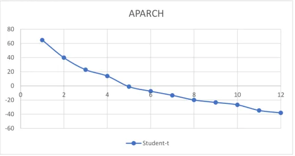
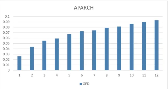
4.5 Predictive Power

While MSE is used as a method to evaluate the forecast accuracy of the models at different horizon, Predictive Power (𝑃) is employed in this paper to examine how much a predicted volatility can explain the actual volatility. This procedure further also allows to investigate how well the models complement for predicting volatility over subsequent horizons for the return data rather than just measuring and comparing among the forecast models.

The method proposed by Blair, Poon, and Taylor (2001) is used in this thesis where they define, 𝑃 to measure explanatory power. 𝑃 is given as:

𝑃 = 1 −∑ (𝜎𝑖− 𝜎̂𝑖) 2 𝑛 𝑖=1 ∑𝑛𝑖=1(𝜎𝑖− 𝜎̅)2 (29) Where,

𝑛 is the number of out-of-sample observations 𝜎_𝑖 is the proxy realized volatility for ith observation 𝜎̂𝑖 is the forecasted volatility for ith observation

𝜎̅ is the mean value of volatility

𝑃 is the comparison between the sum of squared prediction errors and the sum of squared variations of 𝜎_𝑖. The value of 𝑃 can be both negative and positive. Relatively small value for 𝑃, closer to 1 (multiplied by 100 in this paper) is desirable for a forecast model indicating that the prediction error are relatively small which represents forecast errors have lesser variation than the actual volatility. The negative value is undesirable since it reflects greater variation of forecast errors than actual volatility (Poon and Granger, 2003).

40

5. Empirical Results

The first-order GARCH model (𝑝 = 1 and 𝑞 = 1) is chosen for the study as it is evident from many researches (see Hsieh (1991), Zivot (2008) and Hansen and Lunda (2004)) that it has been proven adequate to model and forecast financial time series. However, it is hard to find researches that emphasize on appropriate error distribution assumption to model the financial time series. Klar et al. (2012) states that application of inappropriate error distribution assumption could lead to substantial loss of efficiency of the corresponding estimators. Thus, three different (Normal, Student-t and GED) most used distribution assumptions are correspondingly used with first order GARCH models for all asset classes. Each asset class consist of two time series data which makes our analysis comparable within and among the asset classes. The in-sample parameter estimation and out-of-sample forecast comparison is presented and discussed below. The notations follows Section 3.

5.1 In-Sample Estimation

The full in-sample parameters estimates for Stock Indices (S&P500 and DJIA), Interest rates (CBOE (^TNX), CBOE (^FVX)) and Exchange rates (USD/CHF and GBP/CHF) are presented in Table 6 to Table 11. The parameters 𝜇, 𝛼, 𝛽, 𝛾, 𝛿 and 𝑣 are discussed considering traditional significance level, 5%. It is important to note that 𝛿 is unique to only APARCH model while GARCH model excludes two parameters 𝛾 and 𝛿. Akaike's information criterion (AIC), Schwarz’s Bayesian information criterion (BIC), and the Hannan and Quinn information criterion (HQIC) are presented to evaluate the model fit. ARCH-LM test statistics is presented to see if ARCH effect still exists after modeling for volatility or not.

41 5.1.1 Stock Indices

S&P500

From Table 6, for S&P500, the intercept shown by 𝜔 for all models are close to zero as expected. The 𝜔 is statistically significant at 5% level only for EGARCH and GJR-GARCH model under all distribution.

Table 6 shows parameter 𝛼 is statistically significant at 5% level for GARCH, EGARCH and APARCH models for all distribution but not statistically significant for GJR-GARCH model under all distributions. This signifies the presence of volatility clustering in GARCH, EGARCH and APARCH models. For these models conditional volatility tends to rise when the absolute value of standardized residuals is large and vice versa.

The coefficient of 𝛽 for all the models are statistically significant. There exists covariance stationary and strong volatility persistence for all models as (𝛼 + 𝛽) for GARCH model, 𝛽 for EGARCH model and (𝛼 + 𝛽 + (𝛾/2)) for GJR-GARCH and APARCH model are very close to one. But the persistent of volatility can be considered inconclusive for GJR-GARCH model as 𝛼 was found to be statistically insignificant. Such high persistence closer to one also indicates slow decay of volatility shocks.

The asymmetry and leverage effect shown by 𝛾 is positive and statistically significant at 5% level for all the models. However, for the existence of leverage effect it is important to note that 𝛾 > 0 for GJR-GARCH and APARCH models and 𝛾 < 0 for egarch model. In view of the statistically significant positive 𝛾, the hypothesis for leverage effect is accepted for GJR-GARCH and APARCH models but not EGARCH model for all distribution. Asymmetry effect however exists for all models as 𝛾 ≠ 0.

The values for AIC, BIC and HQIC have lowered for all models as we move from normal distribution to student-t or from normal distribution to GED. This shows the improvement in model fit of non-normal distribution over normal distribution. The ARCH-LM test for all models reveal the absence of ARCH effect.

42 DJIA

From Table 7, the 𝜔 for all the models are close to zero and statistically significant at 5% level except for GARCH and APARCH model under all three distribution. Similar to S&P500, there is the presence of volatility clustering only in GARCH, EGARCH and APARCH model for all distribution as they are all statistically significant for 𝛼. The 𝛽 for all models are statistically significant. The persistence for all models are again close to one showing slow decay of volatility shocks. However, the results are inconclusive for GJR-GARCH model under all distribution as its 𝛼 is not significantly different from zero. The 𝛾 for all the models are positive and statistically significant. Thus, it can be inferred that leverage effect exists for GJR-GARCH and APARCH models but not EGARCH model. However, 𝛾 ≠ 0 represents presence of asymmetry effect in EGARCH, GJR-GARCH and APARCH models.

Similar to S&P 500, AIC, BIC and HQIC reflects improvement in model fit of normal distribution over non-normal distributions for all models. The ARCH-LM test reveals the absence of ARCH effect.

5.1.2 Interest Rates

CBOE (^TNX)

From Table 8, The 𝜔 for all the models are closer to zero and are statistically significant at 5% level only for EGARCH model under all three distribution. The 𝛼 is statistically significant for all models showing the presence of volatility clustering in all models. The 𝛽 for all models are also statistically significant. There exists covariance stationary and strong volatility persistence as the persistence values for all models are very close to one reflecting slow decay of volatility shocks. The coefficient for 𝛾 are all positive and statistically significant representing the existence of leverage effect for GJR-GARCH and APARCH model under all three distribution. However, asymmetry effect is true for all models as 𝛾 ≠ 0.

AIC, BIC and HQIC reflects improvement in model fit of normal distribution over non-normal distribution for all models. The ARCH-LM test reveals the absence of ARCH effect.