Can Gamut Mapping Quality Be Predicted by Colour Image
Difference Formulae?
Eriko Bando*, Jon Y. Hardeberg, David Connah
The Norwegian Color Research Laboratory, Gjøvik University College, Gjøvik, Norway
ABSTRACTWe carried out a CRT monitor based psychophysical experiment to investigate the quality of three colour image difference metrics, the CIEǻE ab equation, the iCAM and the S-CIELAB metrics. Six original images were reproduced through six gamut mapping algorithms for the observer experiment. The result indicates that the colour image difference calculated by each metric does not directly relate to perceived image difference.
Keywords: Colour image difference, CRT display, S-CIELAB, iCAM, CIELAB, GMA 1. INTRODUCTION
Digital imagery has become one of the major image reproduction methods, and according to the diversity of imaging methods, there is a strong need to quantify how reproduced images have been changed by the reproduction process and how much of these changes are perceived by the human eye
A traditional colour difference equation, the CIELAB ǻEab colour difference formula, is still the most widely used as a
colour difference metric in the graphic arts industry, although it was designed to derive colour difference for a single pair of colour patches. As a result, a pixel by pixel ǻEab calculation is not able to predict perceived image difference.
Therefore, several digital image distortion metrics, which are designed to take into account more characteristics of the human visual system, have been researched and developed over recent years. In this experiment, we consider two perceptual image metrics as well as the CIELAB ǻEabcolour difference formula. The S-CIELAB ǻE metric [1] is an
extension of the CIELAB ǻEab metric, and the aim of S-CIELAB is to take into account the spatial-colour sensitivity of
the human eye. One of the most recently developed image appearance models is iCAM [2, 3]. It is based on the S-CIELAB spatial vision concepts, but incorporates more sophisticated models of chromatic adaptation. It is also simpler than other multi-scale observer models, which can be computationally complex.
Colour image difference metrics have complicated structures because they must include various factors that change image appearance, such as colour, noise, sharpness, as well as viewing conditions, illumination level, texture, sample size etc. However, those factors have not been fully adapted into current colour image difference metrics, because there is no clear definition of what weight should be given to each, and what is the best metric and acceptable threshold for each.
In this paper we describe experiments to test whether image-difference metrics can be used to assess the quality of a gamut-mapping procedure. Initially we describe a psychophysical experiment to determine the relative quality of 6 gamut mapping algorithms for mapping 6 different images onto a printer gamut. We then apply the colour image difference metrics to the same images and investigate the possibility of correlations between the experimental data and the image difference metric calculations.
2. EXPERIMENTAL SETUP
A paired image comparison on a CRT monitor is adopted as the method of psychometric scaling for this experiment. Six sRGB images, used in previous gamut mapping research [4], were selected (Figure 1). Each original image has been reproduced by six different gamut mapping algorithms (Table 1), so that a total of 42 images (6 originals and 36 reproductions) were used for the paired image comparison. The destination gamut for each of the gamut mapping algorithms was that of a HP Color LaserJet Printer 4550 PS. printer. Two pairs of images were displayed in each trial, hence, the observers judged 4 images (2 pairs) simultaneously. Each pair consisted of one original and one reproduction and the position of original and reproduction was changed randomly to avoid the observer adapting to the original image. The observer was then asked which pair showed the least difference, i.e. which reproduction was closest
to the original. The same pairs were shown twice to confirm the repeatability. Therefore a total of 180 comparisons were made per observer.
A total of 16 observers, 5 females and 11 males with ages ranging from 22 to 44, participated in the experiment. The observers were asked to take a colour deficiency test before the experiment. The observers sat on a chair which was placed 35 inches away from the monitor [5] and were asked to view the monitor’s grey background for 2 minutes to adapt to the viewing conditions. A Dell 18-inch monitor with a resolution of 16001200 pixels was used to display the images, and its white point was set to D65. The monitor wascalibrated daily during the experiment, and the monitor’s ICC profile was used to transform the CRT’s RGB primaries to CIE tristimulus values. The experiment was carried out in a dark room and the viewing angle for the monitor was about 23 degrees (Figure 2).
1. Camera 2. Girl
3. Cat 4. Pollution
5. Ski 6. Picnic
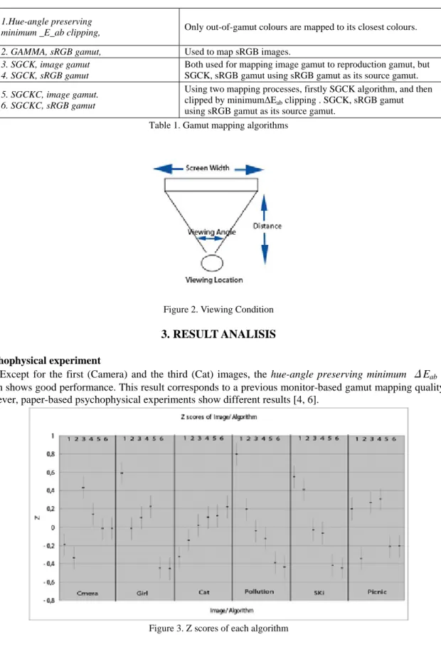
1.Hue-angle preserving
minimum _E_ab clipping, Only out-of-gamut colours are mapped to its closest colours.
2. GAMMA, sRGB gamut, Used to map sRGB images.
3. SGCK, image gamut 4. SGCK, sRGB gamut
Both used for mapping image gamut to reproduction gamut, but SGCK, sRGB gamut using sRGB gamut as its source gamut. 5. SGCKC, image gamut.
6. SGCKC, sRGB gamut
Using two mapping processes, firstly SGCK algorithm, and then clipped by minimumǻEab clipping . SGCK, sRGB gamut
using sRGB gamut as its source gamut. Table 1. Gamut mapping algorithms
Figure 2. Viewing Condition 3. RESULT ANALISIS 3.1 Psychophysical experiment
Except for the first (Camera) and the third (Cat) images, thehue-angle preserving minimum ǍEab clipping algorithm shows good performance. This result corresponds to a previous monitor-based gamut mapping quality survey [6], however, paper-based psychophysical experiments show different results [4, 6].
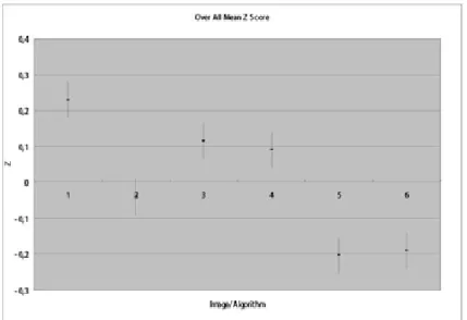
Figure 4. Overall Z score
According to the overall z-score, the hue-angle preserving minimumǍEab clipping algorithm seems to perform the best, followed by theSGCKC algorithms.
3.2 Image difference calculation
All the reproduced images’ differences were computed using three different equations: iCAM, S-CIELAB Ǎ
Es and CIELAB ǍEab. These metrics each compute a pixel by pixel image difference, resulting in an image difference
map for each metric. To compare results from these metrics with the single-figure z-scores we calculate the mean and maximum error for each image difference map. We selected the Girl image as the example for further discussion, because this image is representative of the overall z-scores (Figures 3 and 4).
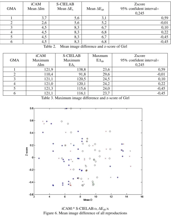
The computed mean image difference values of the Girl image are shown in Figure 5 and Table 2. We did not find any correspondence between any of the three image difference metrics and the z-scores from the psychophysical experiments. The overall results are plotted in Figure 6; the results from CIELAB, iCAM and S-CIELAB are all variable, and there is no significant difference between them. For example, we can see that in Tables 2 and 3, the mean and maximum image differences of theSGCKalgorithms and theSGCKC algorithms are very close, but the difference between those two algorithms’ z-scores is quite large. This suggests that the observers’ perceived image difference does not relate to average or maximum pixel by pixel differences. As a second example, theSGCK algorithm, when executed prior to the minimum ǻEab clipping algorithm, does not influence pixel by pixel based image difference but does influence perceived image quality.
iCAM:*, S-CIELAB:o,ǻEab:x
GMA iCAM MeanǻIm S-CIELAB MeanǻEs MeanǻEab Zscore 95% confident interval= 0,245 1 3,7 5,6 3,1 0,59 2 2,6 5,6 5,2 -0,01 3 4,5 8,3 6,7 0,10 4 4,5 8,3 6,8 0,22 5 4,5 8,3 6,7 -0,45 6 4,5 8,3 6,8 -0,45
Table 2. Mean image difference and z-score of Girl
GMA iCAM Maximum ǻIm S-CIELAB Maximum Eǻs Maxmum Eǻab Zscore 95% confident interval= 0,245 1 121,9 138,8 23,6 0,59 2 110,4 91,8 29,6 -0,01 3 121,1 120,5 24,5 0,10 4 121,0 120,1 24,2 0,22 5 121,3 115,6 24,0 -0,45 6 121,1 116,1 23,7 -0,45
Table 3. Maximum image difference and z-score of Girl
iCAM:* S-CIELAB:o,ǻEab:x
Figure 6. Mean image difference of all reproductions
3.3 Hypothesis
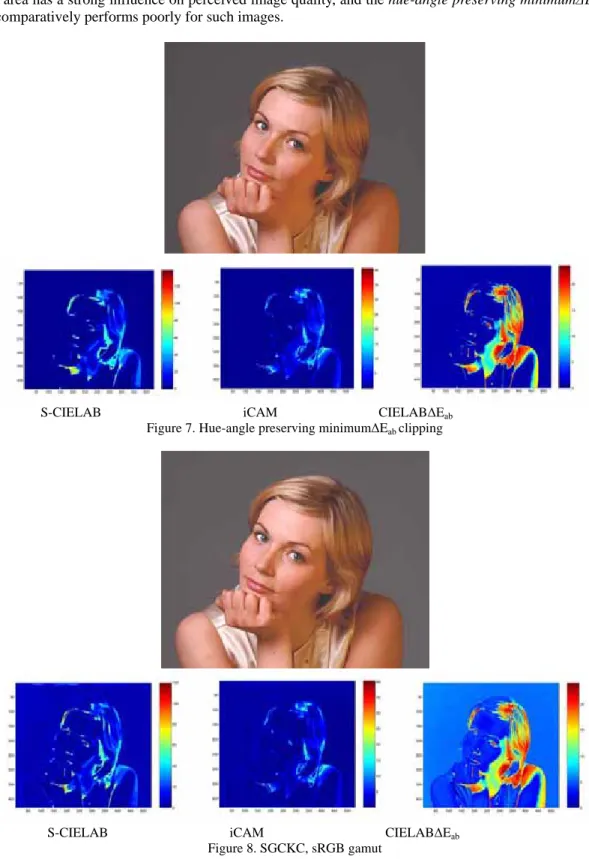
The following Figures 7 and 8 give the image difference maps for the hue-angle preserving minimum ǻEab clipping (the overall best result, Figure. 4) and theSGCKC, sRGBgamut mapping algorithms (the overall worst result, Figure. 4). Note: we have to take into account that iCAM’s unit of image difference is different, because it uses IPT as the colour space, instead of CIELAB. Tables 2 and 3 show the computed mean and maximum image difference values together with the z-scores. The best GMA and the worst GMA have a large z-score difference, and each image difference metric also predicts a closer match between for the best GMA compared to the worst. However, the second best (closely followed by the third) GMAs still show a remarkable difference from the worst GMA, even though their mean and maximum difference values are almost identical. That is, one of, or a combination of, particular area/colour/texture has an influence on image quality. For instance, both the Cat and Camera image show an atypical
result (Figure 3), in that the hue-angle preserving minimum ǻEab clipping algorithm does not work well. Those two images have fine detail on a very dark (achromatic) background in common. This also suggests that a large, dark, achromatic area has a strong influence on perceived image quality, and the hue-angle preserving minimumǻEab clipping
algorithm comparatively performs poorly for such images.
S-CIELAB iCAM CIELABǻEab
Figure 7. Hue-angle preserving minimumǻEabclipping
S-CIELAB iCAM CIELABǻEab
Figure 8. SGCKC, sRGB gamut
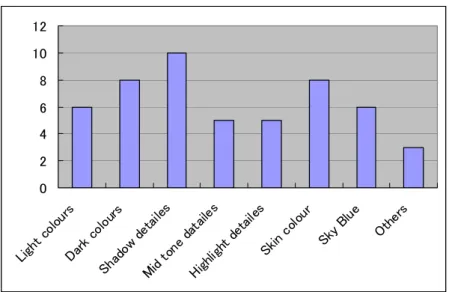
All observers were asked to select 3 most important judgment criteria from 8 options (in random order): Light colours, Dark colours, Shadow details, Mid tone details, Highlight details, Skin colour, Sky Blue and Others (Figure 9).
㪇 㪉 㪋 㪍 㪏 㪈㪇 㪈㪉 㪣㫀㪾㪿㫋 㩷㪺㫆㫃 㫆㫌㫉㫊 㪛㪸㫉㫂 㩷㪺㫆㫃 㫆㫌㫉㫊 㪪㪿㪸㪻 㫆㫎㩷㪻 㪼㫋㪸㫀㫃㪼 㫊 㪤㫀㪻㩷㫋㫆 㫅㪼㩷㪻 㪸㫋㪸㫀㫃㪼 㫊 㪟㫀㪾㪿 㫃㫀㪾㪿㫋 㩷㪻㪼㫋 㪸㫀㫃㪼㫊 㪪㫂㫀㫅 㩷㪺㫆㫃 㫆㫌㫉 㪪㫂㫐㩷 㪙㫃㫌㪼 㪦㫋㪿㪼㫉 㫊
Figure 9. Judgment Criteria
The results show that shadow details, dark colours and skin colour are relatively important factors, and this result corresponds to the above stated hypothesis. Therefore, we computed area based image difference of the Girl image, which represent the overall result and the Camera image, which is an example of an image with fine detail on a very dark (achromatic) background. For the Camera image the observers specifically noted the green area in the middle of the picture and the presence of fine detail in the bottom left corner were important factors in their judgements.
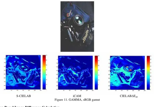
S-CIELAB iCAM CIELABǻEab
S-CIELAB iCAM CIELABǻEab
Figure 11. GAMMA, sRGB gamut
3.5 Area Based Image Difference Calculation
Following the results from the previous sections, we would like to investigate if calculated differences from particular areas of the images correspond to observer judgments. To achieve this, the Girl and the Camera images are divided into 4 areas (Figure 12 -13) according to the result of the observers’ three most used criteria and mapped difference. These areas are shown as white areas in Figures 7 - 11. We then repeat the image difference calculations, but for each region individually instead of the whole image, and compare these calculated differences with observer judgments.
Face Face Shadow Background Hand Figure 12. The 4 areas of the Girl image used in the area-based difference calculation.
Lens Camera Bag Background Dark Details Figure 13. The 4 areas of the Camera image used in the area based difference calculation
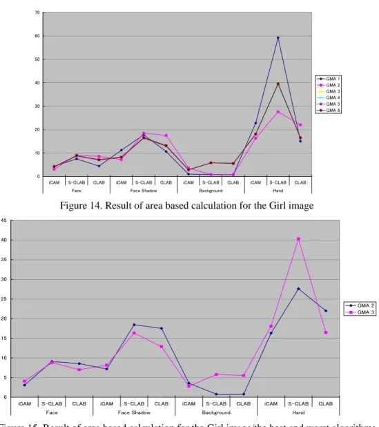
3.5.1 The Girl Image
The best algorithm from the observer judgements (Hue-angle preserving minimumǻEab clipping: GMA 1) does not always show the minimum image difference for iCAM and S-CIELAB, whereas CIELAB always chooses this as the best image. Apart from that, GMA 2 performs irregularly, but there are no noticeable differences between GMA 3-6 (the worst GMAs from the observer data are 5 and 6). S-CIELAB predicts a very large difference for the small area, called “Hand”, although this area is very small, also it might attract limited attention given by observers, but the
influence of such a large difference may affect the overall mean difference.
㪇 㪈㪇 㪉㪇 㪊㪇 㪋㪇 㪌㪇 㪍㪇 㪎㪇 㫀㪚㪘㪤 㪪㪄㪚㪣㪘㪙 㪚㪣㪘㪙 㫀㪚㪘㪤 㪪㪄㪚㪣㪘㪙 㪚㪣㪘㪙 㫀㪚㪘㪤 㪪㪄㪚㪣㪘㪙 㪚㪣㪘㪙 㫀㪚㪘㪤 㪪㪄㪚㪣㪘㪙 㪚㪣㪘㪙 㪝㪸㪺㪼 㪝㪸㪺㪼㩷㪪㪿㪸㪻㫆㫎 㪙㪸㪺㫂㪾㫉㫆㫌㫅㪻 㪟㪸㫅㪻 㪞㪤㪘㩷㪈 㪞㪤㪘㩷㪉 㪞㪤㪘㩷㪊 㪞㪤㪘㩷㪋 㪞㪤㪘㩷㪌 㪞㪤㪘㩷㪍
Figure 14. Result of area based calculation for the Girl image
㪇 㪌 㪈㪇 㪈㪌 㪉㪇 㪉㪌 㪊㪇 㪊㪌 㪋㪇 㪋㪌 㫀㪚㪘㪤 㪪㪄㪚㪣㪘㪙 㪚㪣㪘㪙 㫀㪚㪘㪤 㪪㪄㪚㪣㪘㪙 㪚㪣㪘㪙 㫀㪚㪘㪤 㪪㪄㪚㪣㪘㪙 㪚㪣㪘㪙 㫀㪚㪘㪤 㪪㪄㪚㪣㪘㪙 㪚㪣㪘㪙 㪝㪸㪺㪼 㪝㪸㪺㪼㩷㪪㪿㪸㪻㫆㫎 㪙㪸㪺㫂㪾㫉㫆㫌㫅㪻 㪟㪸㫅㪻 㪞㪤㪘㩷㪉 㪞㪤㪘㩷㪊
㩷 GMA 1 GMA 2 GMA 3 GMA 4 GMA 5 GMA 6 iCAM 4,4 3,1 4,1 4,1 4,1 4,1 S-CLAB 7,5 9,1 8,8 8,9 8,7 8,9 Face 㩷 CLAB 4,4 8,5 7,0 7,1 7,0 7,2 iCAM 11,2 7,2 8,2 8,3 8,2 8,3 S-CLAB 17,8 18,4 16,3 16,4 16,3 16,6 Face Shadow 㩷 CLAB 10,6 17,5 12,9 12,9 12,9 13,2 iCAM 1,0 3,6 2,8 2,8 2,8 2,8 S-CLAB 0,9 0,8 5,8 5,8 5,8 5,8 Background 㩷 CLAB 0,7 0,8 5,5 5,6 5,5 5,6 iCAM 22,8 16,3 18,1 18,2 18,1 18,1 S-CLAB 59,2 27,6 40,3 40,2 39,6 39,6 Hand 㩷 CLAB 15,0 22,0 16,5 16,4 16,4 16,5 Table 4. Result of area based mean difference calculation for the Girl image 3.5.2 The Camera Image
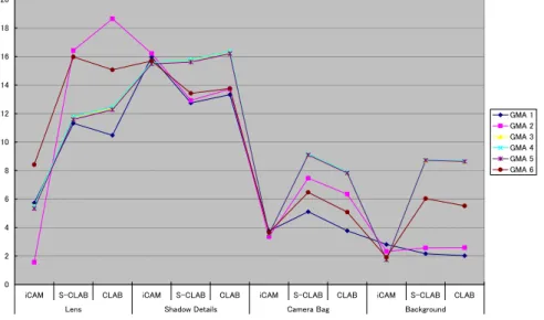
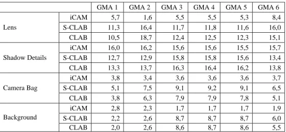
Even though the observers' criteria for image quality judgment state that "dark colours" and "shadow details" are important, the colourful green lens area is also noticeable in the centre of the Camera image. Figure 16 shows the results for all the GMAs and all the areas of the Camera image. The psychophysical results suggest that SGCK, image (GMA 3) is the best algorithm for the Camera image and that the GAMMA, sRGB algorithm (GMA 2) is the worst for this image. S-CIELAB and CIELAB suggest GMA 2 has bigger difference in the lens area, but the rest of the areas (dark achromatic or less chromatic) indicate that GMA 2 has less difference than GMA3 does. On the other hand, iCAM performs differently; iCAM gives that GMA 2 has the smallest mean difference of the all 6 GMAs in the lens area. For other image areas iCAM predicts that there is no difference between the GMAs. CIELAB and S-CIELAB work similarly to each other in the Camera image. In this image, iCAM predicts that GMA 2 gives a smaller difference than the other GMAs in the lens area. iCAM also shows all GMAs have no difference in the rest of the regions (dark achromatic or less chromatic). However, although iCAM gives different results from the other metrics, there are no clear results to indicate that iCAM, S-CIELAB and CIELAB predict perceived image difference.
㪇 㪉 㪋 㪍 㪏 㪈㪇 㪈㪉 㪈㪋 㪈㪍 㪈㪏 㪉㪇 㫀㪚㪘㪤 㪪㪄㪚㪣㪘㪙 㪚㪣㪘㪙 㫀㪚㪘㪤 㪪㪄㪚㪣㪘㪙 㪚㪣㪘㪙 㫀㪚㪘㪤 㪪㪄㪚㪣㪘㪙 㪚㪣㪘㪙 㫀㪚㪘㪤 㪪㪄㪚㪣㪘㪙 㪚㪣㪘㪙 㪣㪼㫅㫊 㪪㪿㪸㪻㫆㫎㩷㪛㪼㫋㪸㫀㫃㫊 㪚㪸㫄㪼㫉㪸㩷㪙㪸㪾 㪙㪸㪺㫂㪾㫉㫆㫌㫅㪻 㪞㪤㪘㩷㪈 㪞㪤㪘㩷㪉 㪞㪤㪘㩷㪊 㪞㪤㪘㩷㪋 㪞㪤㪘㩷㪌 㪞㪤㪘㩷㪍
GMA 1 GMA 2 GMA 3 GMA 4 GMA 5 GMA 6 iCAM 5,7 1,6 5,5 5,5 5,3 8,4 S-CLAB 11,3 16,4 11,7 11,8 11,6 16,0 Lens CLAB 10,5 18,7 12,4 12,5 12,3 15,1 iCAM 16,0 16,2 15,6 15,6 15,5 15,7 S-CLAB 12,7 12,9 15,8 15,8 15,6 13,4 Shadow Details CLAB 13,3 13,7 16,3 16,4 16,2 13,8 iCAM 3,8 3,4 3,6 3,6 3,6 3,7 S-CLAB 5,1 7,5 9,1 9,2 9,1 6,5 Camera Bag CLAB 3,8 6,3 7,9 7,9 7,8 5,1 iCAM 2,8 2,3 1,7 1,7 1,7 1,9 S-CLAB 2,2 2,6 8,7 8,7 8,7 6,0 Background CLAB 2,0 2,6 8,6 8,7 8,6 5,5 Table 5. Result of area based mean difference calculation for the Camera image
4 CONCLUSIONS
We carried out a psychophysical experiment to test whether image-difference metrics can be used to assess the quality of a gamut-mapping procedure. Firstly, the results of this experiment were compared with the computed mean differences produced by iCAM, S-CIELAB and CIELAB equations, secondly we investigated the images in particular areas which represent characteristics of each scene.
We do not find a correlation between the perceived image differences and pixel by pixel image difference calculation values, even in the particular factors of large achromatic area, dark area with fine details and skin tones, but this also means that there are potential improvements for iCAM and S-CIELAB. We found that 4 of 6 reproduced images for each scene have almost identical computed difference values, although observers detect the difference between those algorithms. The observer’s criteria did not seem to be not related to the image difference calculations, but those factors must be adopted in the image difference equations.
Further research will be carried out with all images, in the subjects of image difference and image quality metrics, perceptual difference in different media, factors that made observers prefer particular images e.g.
background/texture/contrast sensitivity effect, the correlation between the human vision error prediction, the image difference map and human eye’s dwell time on objects in images .
ACKNOWLEDGEMENTS
The authors would like to thank Professor Lindsay MacDonald for his advice, Garrett Johnson for providing iCAM and S-CIELAB MATLAB codes, Morten Amsrud who kindly helped to reproduce images, Ivar Farup and Øivind Kolloen for Java programming help.
REFERENCES
[1] X. Zhang, B. A. Wandell, “A spatial extension of CIELAB for digital color image reproduction”,SID Journal , (1997).
[2] M. D. Fairchild, G. Johnson, “Meet iCAM: A Next-Generation Color Appearance Model”, IS&T/SIT Tenth Color Imaging Conference, pp. 33-38, Arizona, USA (2002).
[3] M. D. Fairchild and G.M. Johnson, “The iCAM framework for image appearance, image differences, and image quality,” Journal of Electronic Imaging, in press (2004).
[4] I. Farup, J. Y. Hardeberg, and M. Amsrud, “Enhancing the SGCK Colour Gamut Mapping Algorithm”, CGIV 2004, pp.520-524, Aachen, Germany (2004).
[6] P. J. Green, L. W. MacDonald, “Colour Engeneering”, Jon Wiley & Sons, ltd, West Sussex, England (2002). *[email protected]; Phone +47 6113 5100