Stream-dashboard : a big data stream clustering framework with applications to social media streams.

(1)

University of Louisville University of Louisville

ThinkIR: The University of Louisville's Institutional Repository

Electronic Theses and Dissertations

5-2013

Stream-dashboard : a big data stream clustering framework with

applications to social media streams.

Basheer Hawwash 1984- University of Louisville

Follow this and additional works at: https://ir.library.louisville.edu/etd

Recommended Citation Recommended Citation

Hawwash, Basheer 1984-, "Stream-dashboard : a big data stream clustering framework with applications to social media streams." (2013). Electronic Theses and Dissertations. Paper 587.

https://doi.org/10.18297/etd/587

This Doctoral Dissertation is brought to you for free and open access by ThinkIR: The University of Louisville's Institutional Repository. It has been accepted for inclusion in Electronic Theses and Dissertations by an authorized administrator of ThinkIR: The University of Louisville's Institutional Repository. This title appears here courtesy of the

(2)

STREAM-DASHBOARD: A BIG DATA STREAM CLUSTERING

FRAMEWORK WITH APPLICATIONS TO SOCIAL MEDIA

STREAMS

By

Basheer Hawwash

B.A., Jordan University of Science and Technology, 2006 M.S., University of Louisville, 2008

A Dissertation Submitted to the Faculty of

Speed School of Engineering of the University of Louisville in Partial Fulfillment of the Requirements

for the Degree of

Doctor of Philosophy

Department of Computer Engineering and Computer Science University of Louisville

Louisville, KY

(3)

(4)

STREAM-DASHBOARD: A BIG DATA STREAM CLUSTERING

FRAMEWORK WITH APPLICATIONS TO SOCIAL MEDIA

STREAMS

By

Basheer Hawwash

B.A., Jordan University of Science and Technology, 2006 M.S., University of Louisville, 2008

A Dissertation Approved on

April 22, 2013

by the following Dissertation Committee

Dissertation Director: Dr Olfa Nasraoui Dr Ibrahim Imam

Dr. Hichem Frigui Dr. Ming Ouyang Dr. Ayman El-Baz

(5)

DEDICATION

This dissertation is dedicated to my parents

Mr. Zuhair Hawwash

and

Mrs. Aida Hawwash

(6)

ACKNOWLEDGMENTS

I would like to thank my advisor, Dr Olfa Nasraoui, for her inspirational guidance and support, and from whom I gained invaluable knowledge over the years, that would help me better build my career at both personal and academic levels. I would also like to express my deepest thanks to my wife, Aziza, for her support and patience in all the long and endless nights. I would not have finished my dissertation without her encouragement. Also, many thanks to my friends and lab mates at the Knowledge Discovery and Web Mining Lab and to the members of my dissertation committee for their feedback on this work.

Finally, I am grateful that this work was supported by US National Science Foundation Grant IIS-0916489.

(7)

ABSTRACT

STREAM-DASHBOARD: A BIG DATA STREAM CLUSTERING FRAMEWORK WITH APPLICATIONS TO SOCIAL MEDIA STREAMS

Basheer Hawwash

April 22, 2013

Data mining is concerned with detecting patterns of data in raw datasets, which are then used to unearth knowledge that might not have been discovered using conventional querying or statistical methods. This discovered knowledge has been used to empower decision makers in countless ap-plications spanning across many multi-disciplinary areas including business, education, astronomy, security and Information Retrieval to name a few. Many applications generate massive amounts of data continuously and at an increasing rate. This is the case for user activity over social networks such as Facebook and Twitter. This flow of data has been termed, appropriately, aData Stream,and it introduced a set of new challenges to discover its evolving patterns using data mining techniques. Data stream clustering is concerned with detecting evolving patterns in a data stream using only the similarities between the data points as they arrive without the use of any external information (i.e. unsupervised learning).

In this dissertation, we propose a complete and generic framework to simultaneouslymine,track

andvalidateclusters in a big data stream (Stream-Dashboard). The proposed framework consists of

three main components: an online data stream clustering algorithm, a component for tracking and validation of pattern behavior using regression analysis, and a component that uses the behavioral information about the detected patterns to improve the quality of the clustering algorithm. As a first component, we propose RINO-Streams, an online clustering algorithm that incrementally updates the clustering model using robust statistics and incremental optimization. The second component is

(8)

a methodology that we call TRACER, which continuously performs a set of statistical tests using

regression analysisto track the evolution of the detected clusters, their characteristics and quality

metrics. For the last component, we propose a method to build some behavioralprofiles for the clustering model over time, that can be used to improve the performance of the online clustering algorithm, such as adapting the initial values of the input parameters.

The performance and effectiveness of the proposed framework were validated using extensive experiments, and its use was demonstrated on a challenging real word application, specifically un-supervised mining of evolving cluster stories in one pass from the Twitter social media streams.

(9)

LIST OF TABLES

Page

2.1 Sample Contingency Table . . . 26

2.2 Similarity Contingency Table . . . 27

2.3 Common M-estimators and W-estimators (Ricardo A. Maronna, 2006) . . . 54

3.1 Comparison between RINO-Streams and other stream clustering algorithms . . . . 86

3.2 Stream Clustering Algorithm Metrics for ClusterCi . . . 88

3.3 Transition Conditions and Symbols . . . 93

3.4 Transition Characterization Rules (conjunction_∧, disjunction_∨, negation_¬), sorted by the order in which they are applied . . . 93

3.5 Comparison between TRACER and local change detection techniques . . . 101

4.1 Roadmap to the Experiments . . . 111

4.2 RBF Data Stream Generator Parameters (Bifetet al., 2010). . . 113

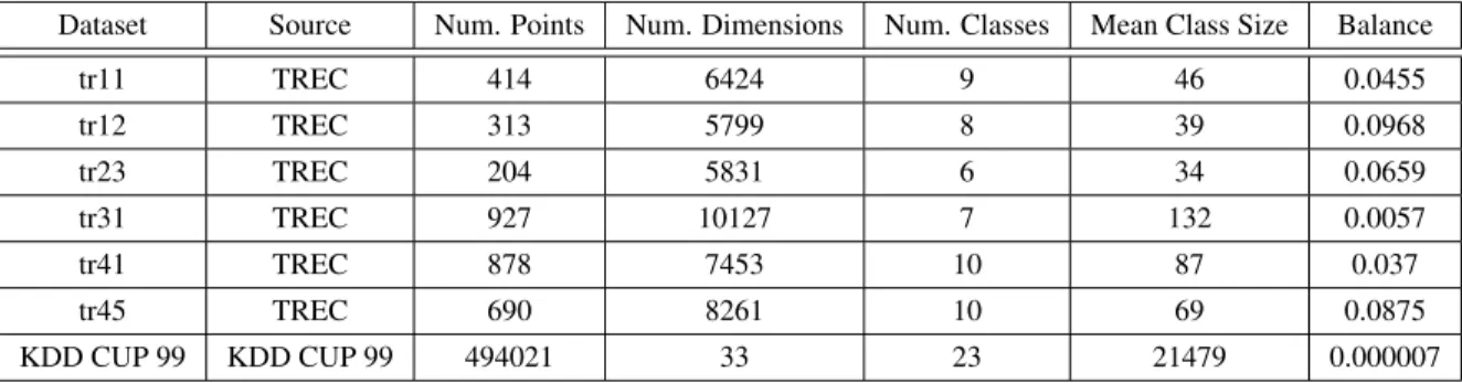
4.3 Real Text and Network Intrusion Detection Data Set Descriptions . . . 114

4.4 RINO-Streams Parameter Values . . . 115

4.5 TRAC-Streams Parameters’ values . . . 116

4.6 CluStream Parameters . . . 116

4.7 Growing K-Means Parameters . . . 116

4.8 DBSCAN’s Optimal Parameters Values . . . 118

4.9 The X-axis index values used in Figures (4.1-4.12) . . . 119

4.10 The meaning of the X-axis index values used in Figures (4.13-4.16) . . . 119 4.11 RINO-Streams vs CluStream vs Growing K-Means: Synthetic Data (Significance) . 136

(12)

4.13 Parameter configurations for cluster splitting and merging . . . 147

4.14 RBF Parameters . . . 149

4.15 ANOVA Table - RINO-Streams versus RBF Generator (Davies-Bouldin) . . . 150

4.16 ANOVA Table - RINO-Streams versus RBF Generator (Silhouette-Index) . . . 150

4.17 ANOVA Table - RINO-Streams versus RBF Generator (Normalized Mutual Infor-mation) . . . 151

4.18 ANOVA Table - RINO-Streams Parameters (Davies-Bouldin) . . . 154

4.19 ANOVA Table - RINO-Streams Parameters (Silhouette Index) . . . 154

4.20 ANOVA Table - RINO-Streams Parameters (Normalized Mutual Information) . . . 155

4.21 RINO-Streams Pareto Frontier . . . 160

4.22 RINO-Streams Default Parameter Values . . . 160

4.23 Dataset Properties & Component 1’s Clustering Algorithms used in our experiments 162 4.24 ANOVA Parameters and their values . . . 162

4.25 TRACER: N-Way ANOVA Results . . . 163

4.26 TRACER: 1-Way ANOVA Results . . . 164

4.27 TRACER: ANOVA Parameters Best Values . . . 164

4.28 Unfiltered Twitter Dataset Properties . . . 184

4.29 Twitter Stories: Sugar Bowl 2013 Topic Cluster Evolution Properties . . . 189

4.30 Twitter Stories: Charlie Strong Topic Cluster Evolution Properties . . . 190

4.31 Twitter Stories: Kevin Ware Injury Topic Cluster Evolution Properties . . . 191

(13)

LIST OF FIGURES

Page

1.1 Motivational Example: Tracking Twitter Trending Topics . . . 3

2.1 LDA Generative Process (Bleiet al., 2003) . . . 63

3.1 Stream Dashboard Flowchart . . . 66

3.2 Consecutive Time Periods (T1& T2) . . . 90

3.3 Cluster Changes: Typical Causes and Effects . . . 91

3.4 Internal & External Transitions . . . 92

3.5 TRACER Example (Source and final output) . . . 97

3.6 TRACER Example (T1 & T2) . . . 97

3.7 TRACER Example (T3 & T4) . . . 98

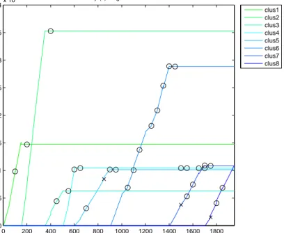
3.8 An example of density regression models of 8 clusters . . . 106

3.9 An example of density stability plots for 8 clusters . . . 107

3.10 Stream-Genealogy Graph . . . 108

4.1 RINO-Streams vs TRAC-Streams: DS8 (difference in number of clusters detected) 120 4.2 RINO-Streams vs TRAC-Streams: DS8 (average centroid error) . . . 121

4.3 RINO-Streams vs TRAC-Streams: DS8 (average scale error) . . . 122

4.4 RINO-Streams vs TRAC-Streams: DS8 (difference in estimated noise) . . . 123

4.5 RINO-Streams vs TRAC-Streams: DS8 (Davies-Bouldin Index) . . . 124

4.6 RINO-Streams vs TRAC-Streams: DS8 (Silhouette Index) . . . 125

4.7 RINO-Streams vs TRAC-Streams: DS16 (difference in number of clusters detected) 126 4.8 RINO-Streams vs TRAC-Streams: DS16 (average centroid error) . . . 127

(14)

4.9 RINO-Streams vs TRAC-Streams: DS16 (average scale error) . . . 128

4.10 RINO-Streams vs TRAC-Streams: DS16 (difference in estimated noise) . . . 129

4.11 RINO-Streams vs TRAC-Streams: DS16 (Davies-Bouldin Index) . . . 130

4.12 RINO-Streams vs TRAC-Streams: DS16 (Silhouette Index) . . . 131

4.13 RINO-Streams vs IncDBSCAN: DS8 & DS16 (relative difference in number of clusters detected) . . . 132

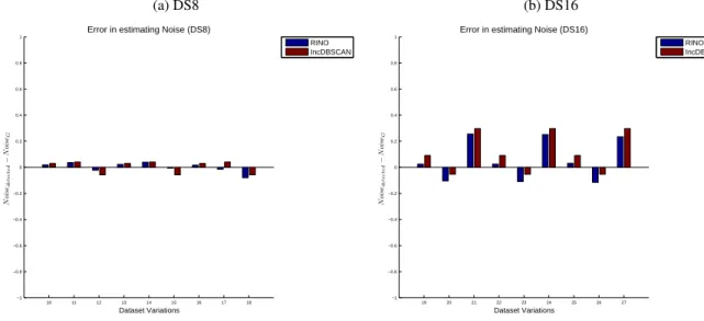
4.14 RINO-Streams vs IncDBSCAN : DS8 & DS16 (difference in estimated noise) . . . 133

4.15 RINO-Streams vs IncDBSCAN: DS8 & DS16 (Davies-Bouldin Index) . . . 133

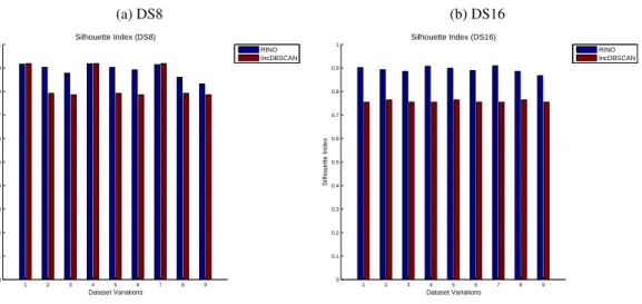
4.16 RINO-Streams vs IncDBSCAN: DS8 & DS16 (Silhouette Index) . . . 134

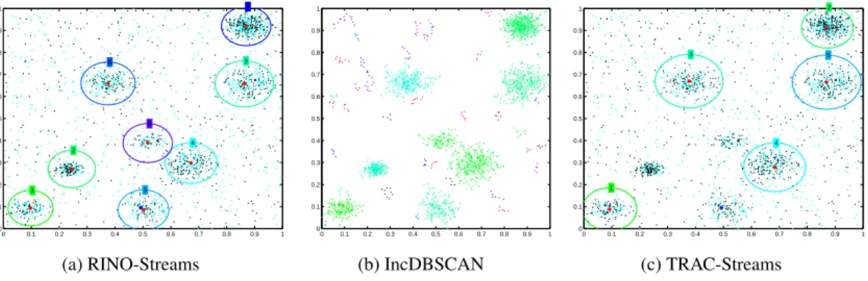
4.17 RINO-Streams vs TRAC-Streams & IncDBSCAN: DS8 (final output for experi-mentC₈RN₂₄) . . . 135

4.18 RINO-Streams vs TRAC-Streams & IncDBSCAN: DS8 (similarity matrices for ex-perimentC8RN24) . . . 135

4.19 RINO-Streams vs TRAC-Streams & IncDBSCAN: DS16 (final output for experi-mentC16RN18) . . . 135

4.20 RINO-Streams vs TRAC-Streams & IncDBSCAN: DS16 (similarity matrices for experimentC16RN18) . . . 136

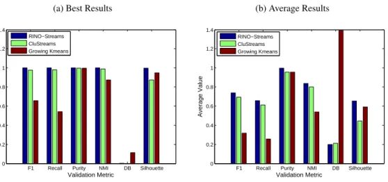
4.21 RINO-Streams vs CluStream vs Growing K-Means: Synthetic Data (Overall Per-formance) . . . 137

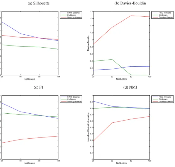
4.22 RINO-Streams vs CluStream vs Growing K-Means: Synthetic Data (Number of Clusters) . . . 138

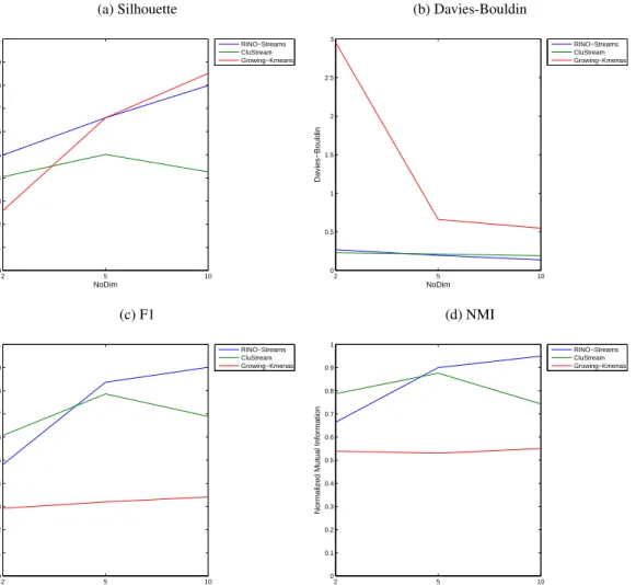
4.23 RINO-Streams vs CluStream vs Growing K-Means: Synthetic Data (Number of Dimensions) . . . 139

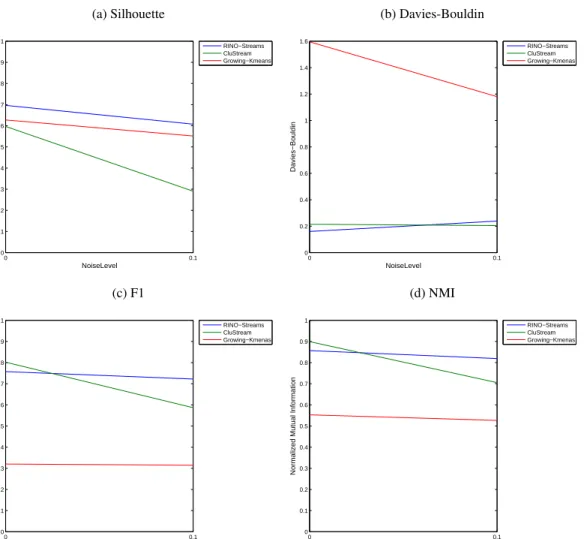
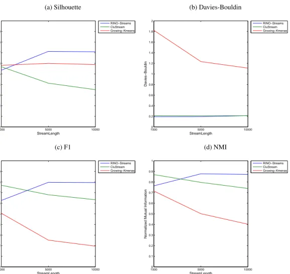
4.24 RINO-Streams vs CluStream vs Growing K-Means: Synthetic Data (Noise Level) . 140 4.25 RINO-Streams vs CluStream vs Growing K-Means: Synthetic Data (Stream Length) 141 4.26 RINO-Streams vs CluStream vs Growing K-Means: Synthetic Data (Time Com-plexity) . . . 141

4.27 RINO-Streams vs CluStream vs Growing K-Means: Synthetic Data (Time Com-plexity with Respect With Data Stream Properties) . . . 142

(15)

4.29 RINO-Streams vs CluStream : TREC (Cluster Purity) . . . 144

4.30 RINO-Streams vs CluStream : TREC (Recall) . . . 144

4.31 RINO-Streams vs CluStream : TREC (F1 Score) . . . 144

4.32 RINO-Streams vs CluStream : TREC (Davies-Bouldin Index) . . . 145

4.33 RINO-Streams vs CluStream : TREC (Time Complexity) . . . 146

4.34 RINO-Streams vs CluStream : KDD CUP 99 (External Validity Metrics) . . . 146

4.35 RINO-Streams vs CluStream : KDD CUP 99 (Time Complexity) . . . 147

4.36 A cluster that gradually splits into three clusters over time . . . 147

4.37 RINO-Streams: Three clusters that gradually merge into one cluster over time . . . 148

4.38 RINO-Streams: Time Complexity on Big Data Streams . . . 148

4.39 The effect of the data stream properties on RINO-Streams output (Part 1) . . . 152

4.40 The effect of the data stream properties on RINO-Streams output (Part 2) . . . 153

4.41 RINO-Stream’s parameter effect on quality of the clusters: Number of Clusters . . 156

4.42 RINO-Stream’s parameter effect on quality of the clusters: Initial Scale . . . 156

4.43 RINO-Stream’s parameter effect on quality of the clusters: Forgetting Factor . . . . 157

4.44 RINO-Stream’s parameter effect on quality of the clusters: Chebyshev Constant for outliers . . . 157

4.45 RINO-Stream’s parameter effect on quality of the clusters: Chebyshev constant for merging . . . 157

4.46 RINO-Stream’s parameter effect on quality of the clusters: Minimum Sum of Weights158 4.47 RINO-Stream’s parameter effect on quality of the clusters: Maturity Age . . . 158

4.48 RINO-Streams Pareto Frontier . . . 159

4.49 DS6: Cardinality vs. Time and its Summary Regression Models . . . 165

4.50 Re0: Density vs. Time and its Summary Regression Model . . . 165

4.51 KDD Cup 99 Network Activity . . . 167

4.52 Cardinality regression models versus the groundtruth cardinality for three main net-work activities . . . 167

4.53 DS1A: Online Validation of the Tracking and Summary of the Cluster Scale Evo-lution using Regression Models against their Ground-truth for two different online clustering algorithms used in Component 1. . . 168

(16)

4.54 DS1: Ground Truth . . . 170

4.55 DS1: Cardinality & Scale Regression Models . . . 170

4.56 DS2A: Dataset Evolution and Final Clustering . . . 171

4.57 DS2A: Validating the Detection and Tracking of a Splitting Transition . . . 171

4.58 DS5: Validating and Tracking the Outputs of Two Different Online Algorithms using Density Regression Models . . . 172

4.59 DS2B: MONIC vs Stream-Dashboard External Changes . . . 174

4.60 DS6: TRACER Compared against Baseline . . . 175

4.61 Effect of the TRACER parameters on milestone detection and regression model quality . . . 176

4.62 Time & Memory Complexity of TRACER . . . 177

4.63 DS6: Stream Genealogy Layout with different filters . . . 178

4.64 DS2B: behavioral trend of a merged cluster and its ancestors . . . 178

4.65 DS10: Density Over time Vs. Regression Models (for experimentC10ON10,ordered data arrival) . . . 179

4.66 DS10: Density Over time Vs. Regression Models (for experimentC10RN10, random data arrival) . . . 180

4.67 DS10: Density Stability Over Time . . . 181

4.68 DS10: Interactive Cluster Ancestry Tree . . . 182

4.69 Twitter Properties . . . 185

4.70 Twitter: Popular Hashtags Per Month . . . 186

4.71 Twitter: Detected Trending Topics for Several Days . . . 187

4.72 Louisville Tweets . . . 188

4.73 Louisville tweets density regression models . . . 188

4.74 Twitter Stories: Sugar Bowl 2013 Topic Cluster Evolution . . . 189

4.75 Twitter Stories: Charlie Strong Topic Evolution . . . 190

4.76 Twitter Stories: Kevin Ware Injury Topic Cluster Evolution . . . 191

(17)

CHAPTER 1

INTRODUCTION AND MOTIVATION

In recent years, there has been a proliferation of applications that generate massive amounts of data continuously and at an increasing rate. This is due, primarily, to the faster and lower cost hardware, the emergence of new paradigms that thrive on user-generated data such as social networks, and the recognition of the importance of utilizing raw data (which was previously useless) in obtaining new information that are vital to deal with a variety of real life issues. These massive amounts of data have been called data streams, and are mainly characterized by a huge throughput and a dynamic nature. Data streams can be found in many applications, such as sensor networks, web logs, computer network traffic, and the activities on mobile phone networks.

To discover useful information out of data streams, classical data mining techniques have been modified and applied on data streams, which caused the emergence of the new discipline of Stream Data Mining (Babcocket al., 2002; Guhaet al., 2003; Stonebrakeret al., 2005; Gaberet al., 2005). Stream data mining is concerned with extracting knowledge represented as a set of patterns in a continuous stream of data, and it is a much more challenging task, than traditional data mining, due to the constraints imposed by the nature of data streams. First, the memory constraints are very tight since storing the whole data stream is not feasible or even possible. Second, as new data arrives, it needs to be processed fast enough to minimize any delays. These constraints on the computational and memory complexity add more challenges in designing stream data mining algorithms. Many researchers have developed stream data mining algorithms to meet these challenges (Aggarwalet al., 2003; Caoet al., 2006; Charikaret al., 2003; Chen & Tu, 2007; Nasraoui & Rojas, 2006).

Stream data mining techniques can be grouped, as in classical data mining techniques, into three main groups: supervised (classification), unsupervised (clustering) and semi-supervised learning.

(18)

The focus of this work is on unsupervised stream data mining, and more specifically, we propose a complete and generic framework to mine, track and validate clusters in big data streams on the fly, which highlights the importance of monitoring the behavior of the evolving clusters rather than simply detecting them.

The remainder of this chapter discusses the motivations behind this work (Section 1.1), presents a statement of the problems to be solved relating to mining and monitoring data stream clusters, the challenges, and the questions that will be answered by solving the stated problems (Section 1.2). This is followed by a list of the contributions of this dissertation (Section 1.3), and finally the organization of this document (Section 1.4).

1.1 Motivation

Most of the research in Stream Data Clustering has focused primarily on detecting the clusters embedded in the data stream and using this knowledge in higher-level applications (e.g. in visual-ization (Leuski & Allan, 1997) or in recommender systems (Sarwaret al., 2002)). However, only a few have focused on tracking the actual evolution of these clusters over time, especially in data streams, where new data arrives with a huge throughput that makes conventional clustering algo-rithms useless. For example, it is estimated that users generate about 500 Million tweets every day1.

Detecting clusters in a data stream, while simultaneously monitoring and tracking their evolu-tion, adds a more challenging but valuable perspective for Stream Data Mining. The discovered clusters provide the tools to help decision makers make a knowledgeable decision. If this task is done periodically (e.g. detecting trending topics in Twitter), then extracting the clusters every time becomes expensive and possibly redundant (e.g. Twitter trending topics do not change, typically, every hour). Hence, the decision makers become familiar with the clusters over time, and become more interested in identifying the changes that took place instead. These changes might occur to the discovered clusters internally (i.e. the characteristics of the cluster) or externally (i.e. interaction of clusters with each other). For example, in customer relationship management, it may be valu-able to know if an emerging pattern of behavior is the result of(i)a completely new group of users

(19)

Figure 1.1: Motivational Example: Tracking Twitter Trending Topics Twitter status for the terms: ‘Arab’ , ‘Revolutions’

Online Clustering Density Tracking & Validating 12/17/10 1/25/11 2/17/11 2/28/11 _X:Time

Tunisian Revolution starts Ben Ali steps down Egyptian Revolution starts Mubarak steps down Libya revolution starts

Cluster 1 : Cluster 2: Cluster 3:

(i.e. emergence of a new pattern), (ii)a shift in a previous group’s behavior (i.e. internal pattern change), or if(iii)it is a mergence of two groups of users that used to have different interests? (i.e. external pattern changes (Nasraouiet al., 2008)). Answering such questions can provide valuable information for planning marketing strategies.

As a motivational example, Figure 1.1 shows how the proposed framework could be applied to a stream of tweets. As an input, a stream of tweets, regarding the revolutions that started in the middle east at the end of 2010 and beginning of 2011, is collected and processed using an online clustering algorithm to find the trending topics (3 topics are shown). The topic metrics, that characterize the topics, are tracked over time. For example, the density (ratio between number of tweets and the variance of the topic) reflects the popularity of the topic (i.e. as the topic becomes popular, its density increases). Some of the critical events (i.e. milestones) during the time periods are annotated using circles and are defined in the legend. It can be seen that the topics became viral at major events, which reflects the twitter community’s reaction to those events. Tracking the evolution of the topics, and detecting the major events automatically, provides important insights about these topics and how society reacts to them.

State of the art approaches, which will be discussed in Section 2.3, try to track the evolution of clusters by finding the differences or deviations between two clustering models at two different time periods. However, this implies that re-clustering the data is needed at each time stamp, which would

(20)

increase the time complexity and is not scalable enough to handle data streams. Moreover, only few of those approaches can detect internal and external changes that might take place at the clusters. Another approach to track clusters’ evolution, could be to keep a snapshot of the clustering model at every time stamp or at certain time stamps. However, this approach would increase the memory complexity and defy the scalability requirement in stream data mining. Moreover, selecting the time stamps, at which a snapshot of the clustering model is stored, is a challenging problem.

1.2 Problem Statement

The problems that we attempt to solve in this work are:mining,validatingandtrackingthe evolving clusters that are hidden in a continuous data stream in a single pass over the data. These problems are discussed below.

1.2.1 Detecting clusters in a data stream

Given a data streamX, where a new data point xi arrives at time i, we are interested in detecting

a set of evolving clustersζ (i.e. a clustering model) that reflects theevolving behaviorof the data

stream. Each cluster represents a portion of a the data stream seen so far, where the data points in this portion are more similar to each other than data points in other clusters. Each cluster consists of a set of metrics/properties that distinguish it from other clusters. Such metrics include a cluster representative (i.e. a cluster’s centroid) and scale (i.e. the size of a cluster’s influence area). Data streams are characterized by a dynamic nature, where new clusters emerge, old ones may undergo changes in their metrics (i.e. internal changes), merge together if they become very similar, or split if they become too general (i.e. external changes). Hence, the classical definition of a cluster needs to be modified to capture the evolving clusters in a data stream.

For intuition, a typical example of stream data mining is in the domain of web usage mining, where the webmaster is interested in detecting all the usage/browsing patterns that take place on an e-commerce website that sells different products. Each of the detected usage patterns is considered one cluster, and it may represent a set of products that are related based on the users’ activities and interests, and they provide invaluable information for the webmaster. In fact, this knowledge might help in recognizing which parts of the website are more related to each other, and in turn

(21)

help improve the structure of the website. Another obvious usage is for strategic marketing, where advertisements could be tailored to individual users or groups of users based on their usage patterns. The browsing patterns tend to be dynamic, in the sense that groups of users might change their interests for various internal or external reasons.

1.2.2 Validating evolving data stream clusters

After detecting the clusters, the second problem deals withvalidatingtheir quality. Traditional val-idation methods (Halkidiet al., 2002a,b; Tanet al., 2005) evaluate the clustering results by either

(i) using some external knowledge about what the clustering model should be and comparing it

against the detected clusters, or(ii)by assessing how well the data stream conforms to the detected clusters, or else by judging the clusters’ quality without referring to the data (i.e. internal metrics). For example, the detected clusters should have low similarity with each other (i.e. they are distinct). However, in the evolving data stream scenario, these validation methods are hard to apply because of the evolution of the clusters that can change their properties anytime. For example, if two prod-ucts are known to be similar through external knowledge (e.g. both prodprod-ucts are books about data mining), but over time users show different interests in them for different reasons (e.g. one book receives very low ratings), then these products might be classified in two different clusters. By clas-sical external evaluation metrics, the new two clusters will be misjudged of being of low quality, although they might be truly of high quality and really reflect the needs of the users.

1.2.3 Tracking the evolution of the detected data stream clusters

The final part of the problem deals with trackingthe evolution of the detected clusters. This task is important and helps in validating the clusters, since it provides the means to explore the internal and external quality of each cluster during its entire lifetime. For example, a group of users who are interested in a specific product at some point in time might change their interests and show more interest in a different product. However, both usage clusters may still be completely valid and useful. Moreover, tracking the evolution of clusters helps in detecting the major changes that take place, and possibly support finding the reasons driving these changes. Back to the web usage mining example, introducing a new product or offering a discount on a product might cause major changes in the users’ behavior. Tracking and recording the clusters’ evolution can increase the

(22)

memory overhead needed for storing this enriched cluster model. Hence, we propose a method that is capable of tracking the clusters’ evolution with low memory cost by storing the evolution behavior of clusters only at special moments corresponding to when major changes, that we call

milestones, take place.

1.2.4 Challenges

Besides the main problems that we are trying to solve in this dissertation, our proposed solutions must adhere to the following requirements of mining data streams:

• The huge data throughput makes it hard, if not impossible, to store every single data point and process it, therefore each new data point should be processed,on the fly, only once.

• There is no control or expectation on the order of the data arrival (for example, data points from the same cluster do not have to arrive sequentially one after the other).

• Data streams are unbounded in size, thus imposing severe restrictions on storage capacity.

• Outlier detection is more challenging, since a data point that is flagged as an outlier at the beginning of the data stream might turn out to be part of a cluster that emerges later in the data stream lifetime.

• Validating the clustering model is hard since the input data points are not kept, and only a summary of the data may be maintained. In fact, even if data points were stored, the data stream is expected to continue evolving, hence data points might be assigned to different clusters at different time periods.

• There is no notion of a static cluster model or output. Instead, at any given time or point in the data stream, there is a different cluster model. Hence, which cluster model should be reported?

1.2.5 Questions to be answered through solving the stated problems

By proposing solutions to the stated problems, this dissertation answers the following questions: 1. Whether a single cluster model is a sufficient output of the data stream clustering process?

(23)

2. If not, which cluster model should be reported or stored?

3. If every point in time, throughout the data stream, generates a distinct cluster model, then there is a possibility that the cluster model outputs from clustering will generate their own data stream that will add even more overhead to the entire stream data mining task. To avoid this problem, is there a simple way to summarize the dynamic clustering output for a fast moving data stream?

1.3 Research Contributions

A generic framework

The main contribution of this work is a complete framework to simultaneouslymine,trackand vali-datethe detected clusters in big data streams. The proposed framework, termedStream-Dashboard, makes an emphasis on characterizing and tracking the behavior of the detected clusters’ description and validity metrics in a data stream over time, rather than just detecting the clusters, and it pro-vides the means to investigate the clusters’ evolution characteristics at any point in time. Stream-Dashboard consists of three main components: an online data stream clustering algorithm (Section 3.1), a component for tracking and validation of cluster behavior using regression analysis (Section 3.2), and a component that can exploit the observed clusters’ behavior to improve the quality of the online clustering component (Section 3.3). The framework is generic in the sense thatanyonline clustering algorithm can be used in the first component, in order to detect the clusters. The only requirement is that this online clustering algorithm must be able to quantify the characteristics of the detected clusters via cluster model parameters or metrics.

An online robust stream clustering algorithm

For the first component, we propose the Robust clustering of data streams using INcremental

Optimization algorithmorRINO-Streams(Section 3.1), which is an online clustering algorithm that

incrementally updates the clustering model using robust statistics. RINO-Streams complies with all the requirements of data stream clustering discussed in Section 3.1.10, and is robust to noise thanks to the use of robust statistics, combined with using distribution-independent Chebyshev bounds to

(24)

detect outliers and to detect similar clusters to be merged.

An algorithm for tracking the clustering model behavior using regression analysis and detect-ing milestones

For the second component, we propose an algorithm forTRAcking and validatingClusterEvolution

usingRegression analysisorTRACER(Section 3.2), which is a method that uses regression analysis

to keep track of the evolution of the detected clusters and their metrics through time, and that stores

only milestones corresponding to the occurrence of significant changes in the clusters’ behavior.

Instead of storing an infinite number of summaries of the stream (at each instant or an arbitrary sample of summaries), only temporally salient synopsis snapshots of the stream will be stored to disk when significant changes are detected, together with a model of this change in between consecutive salient snapshots.

Improving the performance of the online clustering algorithm via feedback

Tracking the behavior of the clustering model over time can eventually help in buildingbehavioral

profiles of ’good’ and ’bad’ clusters. These profiles could be used as feedback to improve the

performance of the online clustering model in two aspects: (i) reducing the sensitivity associated with using some of the threshold parameters needed to judge the quality of the clusters, and (ii)

offering better means to initialize the input parameters used within the online clustering algorithm (Section 3.3).

Visualization dashboard

Tracking the evolution of the data stream is presented using adashboard that enables the user to control the input parameters of the framework, displays the changes of the cluster metrics over time, identifies the detected evolution milestones (Section 3.2.3), and creates a genealogy graph of all the clusters detected (Section 3.4).

(25)

1.4 Organization of this Document

The rest of this dissertation is organized as follows: Chapter 2 reviews important research back-ground related to the problems at hand, including state of the art clustering algorithms, clustering validation methods, the issues of stream data mining along with state of the art stream clustering al-gorithms, robust statistics, approaches to track the clusters’ evolution, and ending with an overview of linear regression models and topic modeling. Chapter 3 provides a detailed analysis of the pro-posed framework and its components. Chapter 4 presents the experiments conducted to prove the functionality and effectiveness of the proposed work. Finally, Chapter 5 concludes this dissertation and discusses possible future work.

(26)

CHAPTER 2

BACKGROUND AND RELATED WORK

In this chapter, we will review the background and related work that is related to this dissertation. Section 2.1 provides an overview of unsupervised learning, where we present some of the existing clustering algorithms: Partition-based algorithms (Section 2.1.1), Hierarchical algorithms (Section 2.1.2), Density-based algorithms (Section 2.1.3) and Grid-base algorithms (Section 2.1.4). Section 2.1.5 discusses the issues related to clustering in high dimensions, and Section 2.1.6 lists some of the clustering validation methods used to evaluate the quality of the clustering model. Section 2.2 provides an overview about Stream Data Mining, and it starts by listing the challenges imposed by the stream model and the requirements for algorithms to deal with these challenges (Section 2.2.1). Then we present some state of the art data stream clustering algorithms from two families: One-pass algorithms (Section 2.2.2.1) and Evolving algorithms (Section 2.2.2.2). Section 2.2.3 lists the challenges and approaches to evaluate the detected clusters in data streams.

Section 2.3 discusses the issues related to the problem of tracking the evolution of clusters detected in the data stream, as well as analyzing some of the current research in that field. Section 2.4 reviews some of the essential concepts from the field of Robust Statistics (Ricardo A. Maronna, 2006; Huber, 1981), which are used in developing the online clustering algorithm RINO-Streams (Section 3.1). Section 2.5 reviews Linear Regression Modeling (Chatterjee & Hadi, 2006), which is used in the proposed cluster evolution tracking algorithm, TRACER (Section 3.2). Section 2.6 provides a brief overview about Topic Modeling and presents two of the state-of-the art approaches. Topic Modeling can be used as a pre-processing step to reduce the very high dimensionality of the text data streams, such as Twitter data, which will be used as an application domain in this work. Finally, Section 2.7 presents the summary and conclusions found in this chapter.

(27)

2.1 Clustering Overview

Clustering is the process of grouping data objects based only on the information found in the data that describes the data objects and their relationships (?). Clustering is also called “unsupervised” learning as opposed to “supervised” learning. The latter, also known as classification, corresponds to the case when class prediction models need to be built using a training set of data objects whose label is known (Tanet al., 2005). The goal of clustering is to generate groups of data objects where the data objects in the same group are similar to each other, but are different from the data objects in other groups. Clustering has been studied intensively, with several surveys in (?Berkhin, 2006; Jain, 2010) and has numerous applications in many fields: information retrieval (grouping search results), biology (creating a taxonomy of living things), network security (learning usage groups for detecting anomalous attacks), and in business (building customer profiles) to name a few.

The following sections review several well known clustering algorithms, classified into four main families: partition-based, hierarchical-based, density-based and grid-based algorithms.

2.1.1 Partition-based algorithms

Partition-based clustering techniques divide the data objects into non-overlapping subsets (clusters) such that each data object belongs to one cluster. They achieve this goal by assigning the data objects to the clusters in such a way that it optimizes a certain objective function defined in advance.

K-Means

A well known technique in this category is K-Means (MacQueen, 1967), which starts by first select-ing K initial centroids, where each centroid is a representative of a cluster and whose feature values are equal to the mean of the corresponding features of the data points in that cluster. Each data point is assigned to the closest cluster using some similarity or dissimilarity measure function (typically the Euclidean or L2 distance for numerical data in a Euclidean space), and then each centroid is

updated using the points assigned to its cluster. This process of assigning data points to centroids and updating the centroids is repeated until the centroids converge (i.e. until the objective function converges to an optimum). The K-Means algorithm is listed in Algorithm 1. The time complexity of K-means is linear with the number of data pointsn, and is equal toO(I_×K_×n_×m)whereKis

(28)

Algorithm 1K-Means Algorithm 1. Select K arbitrary initial centroids

2. Assign each data point to its closest centroid

3. Compute the centroids of the new clusters using (2.2)

4. Repeat steps 2 and 3 until the centroids don’t change or the change is below a specified threshold value

the number of clusters,Iis the number of iterations andmis the number of attributes.

The objective function that is optimized is the sum of squared distances (SSE) between each data point and its assigned cluster representative. The objective function is as follows:

SSE=

K

∑

i=1x

∑

∈Ci

dist(ci,x)2 (2.1)

wheredistis the distance between two objects andciis the centroid of clusterCi. The centroid

that minimizes SSE can be found as:

ci=

∑nj=1xj

n (2.2)

wherenis the cardinality of the clusterCi(i.e. number of points assigned toCi).

K-Means is intuitive and easy to implement, but it has serious drawbacks, including the need for selecting the number of clustersK, as well as the initialKcentroids. However, an even harder problem lies at the core of the objective function. The minimization is based on squared distances which magnifies the differences for data points that are located far away from the centroids (i.e. outliers). Thus, there is a bias to make the centroids close to these outlying points, regardless of how representative they are. Hence, K-Means is not robust to noise and outliers. Being distance-based, K-means also forcibly seeks clusters of equal size, scale or width in feature space regardless of any difference in sizes.

Fuzzy C-Means (FCM)

The assignment of each data point to only one cluster, in K-means, was later relaxed in the Fuzzy C-Means (FCM) algorithm developed by Dunn (Dunn, 1973), and later improved by Bezdek (Bezdek,

(29)

Algorithm 2FCM Algorithm

1. Assign initial values to the memberships of all data points 2. Compute the centroids using (2.4)

3. Recompute the membership values using (2.5)

4. Repeat steps 2 and 3 until the centroids don’t change or the change is below a specified threshold value

1981). In FCM, every data point is allowed to have a degree of membership in more than one cluster, and these memberships are constrained to be in the interval [0, 1], and to sum to 1. The memberships give information about the relative closeness between the data point and all the clusters, which is very useful in case of overlapping clusters as in the case of documents (i.e. a document can be in categorized in two categories such as politics and economics). FCM is listed in Algorithm 2.

The objective function for FCM is a modification of K-means’ objective function (2.1) as fol-lows: SSE= K

∑

i=1 n

∑

j=1 µi jmdist(ci,xj)2 (2.3)

where K is the number of clusters, n is the number of data points in each cluster, µ_{i j}m is the

membership of the data pointxj in the clusterCi, andmis an exponent that controls the influence

of the weights and has a value between 1 and∞. Note that setting the exponentmto 0 yields the K-means’ objective function. The centroid that minimizes SSE is given by:

ci=

∑nj=1xjµi jm

∑nj=1µi jm

(2.4)

The memberships are updated after the centroids are updated, and the formula to update the memberships can be derived from (2.3) as follows:

µi j= 1 ∑Kq=1 _dist₍_c i,xj) dist(cq,xj) _m2₋₁ (2.5)

FCM still suffers from most of the problems suffered by K-means. However the use of a fuzzy partition smoothes the search space, thus making optimization easier and therefore better results,

(30)

especially in recovering from bad initializations.

Expectation-Maximization (EM)

The Expectation-Maximization algorithm (EM) (Dempsteret al., 1977), follows an approach close in spirit to K-Means, which can be shown to be a special case of EM (Casella & Berger, 2001). Modeling the dataset as a mixture of data points generated by K distributions with known form, such as Gaussian, EM tries to determine the model parameters,θj, using posterior probabilities to

maximize the likelihood of the data under these estimated model parameters. If the jthdistribution has parameters θj, then prob(xi|θj) is the probability of theith data point coming from the jth

distribution. Each distribution has a weight wj which reflects the probability of being chosen to

generate a data point, and the weights for all distributions sum to 1. IfΘis the set of all parameters,

then the probability of theithobject is given by:

prob(xi|Θ) =

K

∑

j=1

wjprob(xi|θj) (2.6)

If the objects are assumed to be identically generated, then the probability of the data setX (or

thelikelihoodfunction) is the product of the probabilities of each data point:

prob(X_|Θ) = N

∏

i=1 K

∑

j=1 wjprob(xi|θj) (2.7)

whereNis the number of data points.

The posterior probabilities can be viewed as memberships as in FCM, but keeping in mind that, in contrast to FCM, each data point belongs to one cluster only. The step E (Expectation) estimates the posterior probabilities, while the step M (Maximization) updates the parametersΘ, in an iterative

process that finishes when no significant change occurs. EM is listed in Algorithm 3.

The EM algorithm provides a more general representation of data using mixture models, which allows the detection of clusters with different sizes and shapes. Clusters are easier to characterize since they can be described by a small number of parameters. However, EM has a high computa-tional complexity, does not perform well when clusters have low cardinality, and requires estimating the number of models or clusters in advance.

(31)

Algorithm 3EM Algorithm

1. Select an initial set of model parameters (Θ)

2. Expectation Step: Find the probability that each data point belongs to each distribution 3. Maximization Step: Use the probabilities found in the E step to find new estimate of the

model parameters (Θ) that maximize the likelihood (2.7)

4. Repeat steps 2 and 3 until the parameters’ change is below a specified threshold value

2.1.2 Hierarchical algorithms

Hierarchical clustering algorithms (Ward, 1963) generate a ’taxonomy’ of clusters (also known as a dendogram or a cluster tree), which allows exploring data at different levels of clustering granular-ity. There are two main families of hierarchical clustering algorithms: agglomerative (bottom-up) and divisive (top-down). The agglomerative scheme starts with each data point being a cluster, then recursively merges two or more clusters (based on some similarity measure) until a stopping criterion is met. The divisive approach works inversely (top-down), thus beginning with the whole dataset considered as one cluster, and recursively splits appropriate clusters (based on some criterion of cluster quality). In both cases, each step (merging or splitting) represents one stage or level in the hierarchy. The key step in the hierarchical algorithms is the splitting (divisive approach) or the merging (agglomerative approach) of the clusters. The advantage of hierarchical clustering includes the flexibility regarding the level of granularity and the ease of handling any measure of similarity. However, they suffer from some vagueness of termination criteria, and clusters can not be improved once they are constructed (i.e. once a cluster is split or two clusters are merged they cannot be mod-ified). Measures of closeness among clusters are the single linkage (minimum distance between any two points from the clusters), the complete linkage (maximum distance between any two points from the clusters), and variations along these lines, such as the mean or the median of distances. The agglomerative algorithm chooses the two closest groups (according with the above measure) and merges them, whereas the divisive algorithm chooses the cluster to be split that is the biggest in size (or lowest in quality).

(32)

Algorithm 4CURE Algorithm 1. Draw a sample from the dataset 2. Partition the sample intopgroups

3. Cluster each partition into _pqm clusters, which means a total number of clusters equal to m_q

4. Cluster the found m_q clusters intoKclusters

5. Eliminate outliers

6. Assign all (unsampled) remaining data points to the nearest cluster

CURE

(Guhaet al., 1998) introduced the hierarchical agglomerative clustering algorithm CURE (Cluster-ing Us(Cluster-ing REpresentatives). This algorithm achieves scalability by us(Cluster-ing two devices: (i)using a certain number of data points, instead of all of them, to determine the closeness between clusters (data sampling), and(ii)partitioning the data inpgroups, so that fine granularity clusters are con-structed in partitions first. A major feature of CURE is that it represents a cluster by a fixed number of points (medoids) that are well scattered around it instead of using only one point such as the centroid, which makes it possible to detect non-spherical shapes. The distance between two clusters used in the agglomerative process is equal to the minimum of distances between two scattered rep-resentatives. Single and average link closeness is replaced by the representative medoids’ aggregate closeness. CURE employs one additional device: the originally selected scattered points are shrunk to the geometric centroid of the cluster by a user-specified factor, which suppresses the effect of outliers, since outliers happen to be located further from the cluster centroid than the other scattered representatives. CURE is listed in Algorithm 4, whereKis the number of desired clusters,mis the number of data points, pis the number of partitions, andqcontrols the desired number of points in each partition

CHAMELEON

The hierarchical agglomerative algorithm CHAMELEON (Karypis & Kumar, 1999) utilizes dy-namic modeling in cluster aggregation. The first step in CHAMELEON is to represent data items using a k-nearest neighbor graph: each node represents a data item, with an edge between every two

(33)

Algorithm 5CHAMELEON Algorithm 1. Build a k-nearest neighbor graph

2. Partition the graph using a graph partitioning algorithm (Karypis & Kumar, 1998)

3. Merge the small sub-clusters using measures of relative inter-connectivity while preserving cluster self-similarity

4. Repeat step 3 until no more clusters can be merged

nodes if one of them is among the k-most similar points to the other one. The similarity between each pair of clusters is determined using their relative inter-connectivity (the sum of the weights of the edges that connect nodes in both clusters) and their relative closeness (the average similar-ity between the connected nodes in the clusters). CHAMELEON consists of two stages: the first stage uses a graph partitioning algorithm to partition the k-nearest neighbor graph into a large num-ber of small sub-clusters that minimize the relationship among data points in different sub-clusters. In the second stage, an agglomerative process is performed that uses measures of relative inter-connectivity and relative closeness. CHAMELEON is listed in Algorithm 5. The algorithm does not depend on assumptions about the data model, and it was proven to find clusters of different shapes, densities, and sizes in 2D (two-dimensional) space. However, it has problems if the parti-tioning process does not produce valid sub-clusters (i.e. most of the data points in the sub-cluster belong to a true cluster), which is often the case for high dimensional data.

PDDP

(Boley, 1997) proposed the divisive hierarchical algorithm PDDP (Principal Direction Divisive Par-titioning). To split a cluster, the eigenvector with the highest eigenvalue of the covariance matrix is calculated, and this is called the principal direction. Then, all the data points in that cluster are projected on this principal direction, and based on the sign of their projection, they are assigned either to the left or right child (i.e. if the sign is negative then the data point is assigned to the left child, and to the right child otherwise). To reduce the time complexity of finding the eigenvectors, PDDP uses Singular Value Decomposition (SVD) (Golub & Kahan, 1965). To choose which cluster to split next, PDDP uses a scatter value that measures the non-cohesiveness of the cluster, and se-lects the one with the highest scatter value. The authors used the Forbenius norm of the data points

(34)

Algorithm 6DBSCAN Algorithm

1. Label all the data points as core, border, or noise points 2. Remove noise points

3. Add an edge between all core points that are withinεdistance from each other

4. Each group of connected core points is considered a cluster 5. Assign each border point to the cluster of its closest core point

matrix as the scatter value.

2.1.3 Density-based algorithms

For density-based algorithms, the notion of cluster is identified by crowded regions, with a nearest-neighborhood flavor. This notion of dense regions results in discovering clusters with arbitrary shape as opposed to a certain shape (e.g. a hypersphere in the Gaussian model).

DBSCAN

A well known density based algorithm is Density Based Spatial Clustering of Applications with Noise, DBSCAN, (Esteret al., 1996). DBSCAN searches for the regions that have at least a cer-tain number of data point (MinPts), each one no further from the others than a cercer-tain distance (ε-neighborhood). Using these user-defined parameters (MinPts and ε), each point is labeled as

core, border, or noise point based on the distance of the points in itsε-neighborhood. An

incremen-tal version of DBSCAN was proposed in (Esteret al., 1998), where the same technique of detecting dense regions was applied on chunks of data at a time. DBSCAN can detect arbitrary-shaped clus-ters, however, it is very sensitive to the choice of its parameters (MinPts andε) since a small value

of MinPts and ε may result in mislabeling a set of noise points that are close to each other, as a

valid cluster. Moreover, it does not perform well when the clusters vary widely in their densities. Also, its complexity is high, O(N2), whereN is the number of data points. DBSCAN is listed in Algorithm 6.

(35)

Algorithm 7DENCLUE Algorithm

1. Define the density functions of the data points 2. Find the density attractors

3. Associate each data point with a density attractor which would increase their density

4. Define clusters such that each set of points associated to the same density attractor are con-sidered one cluster

5. Discard clusters whose density attractor has a low density (i.e. less than a threshold value) 6. Combine clusters which are connected via a path of high density points

DENCLUE

DENsity based CLUstEring, DENCLUE (Hinneburg & Keim, 1998) models the density at any point in space in terms of individual influence functions, each defined around a specific data point. The overall density of the data at any point in space is defined as the sum of the influence functions of all data points, and the clusters can be determined mathematically as density attractors (local maxima of this overall density function). Determining the density-attractors is done using a hill-climbing procedure guided by the gradient of the overall density function. The first step in DENCLUE is to partition the data set into high-dimensional hypercubes to speed up the calculation of the density function needed in the second step. The next step is the actual clustering, where only the highly populated cubes (and cubes connected to them) are considered to estimate the density function for the data points, and then find the density-attractors (clusters). The attractors determine the actual clusters as the regions that have density greater than a certain threshold. DENCLUE can detect clusters of different sizes and shapes and can handle noise. However, DENCLUE shares some of the limitations of DBSCAN, more specifically it is sensitive to the parameter values, cannot handle clusters with different densities, and has high complexity:O(N log m+m2)whereN is the number of data points andmis the number of the highly populated cubes. DENCLUE is listed in Algorithm 7.

(36)

2.1.4 Grid-based algorithms

Anther way to deal with the clustering problem is by inheriting the topology from the underlying attribute space, and shifting out attention to space partitioning rather than data partitioning, hence grid-based clustering algorithms are sometimes calledspatialclustering algorithms.

STING

The Statistical Information Grid approach to spatial data mining, STING (Wanget al., 1997) con-structs data summaries into rectangular cells and forms a hierarchical tree. Each cell contains sta-tistical information of the points (and child cells) that comprises: number of data points, minimum, maximum, mean, standard deviation, and type of distribution. After constructing the tree, the actual clustering is done in an SQL-style query applied on the tree. The ’WHERE’ section of the clause specifies what conditions the data has to meet. STING starts with the root of the tree and descends one layer at a time. At each layer, it finds all the cells that are relevant to the query with some confidence. For all the relevant cells, it proceeds to their children and does the same process again until the leaves are reached. The clusters are then formed as the regions which are relevant to the query. STING has low complexity,O(K) whereKis the number of grid cells at the lowest level, and is easy to parallelize. However, it can only detect horizontal or vertical cluster boundaries and not those that are diagonal.

WaveCluster

(Sheikholeslamiet al., 2000) proposed WaveCluster, a grid-based clustering algorithm based on the wavelet transformation used in signal processing. The authors consider the multidimensional spatial data as a multidimensional signal and they apply wavelet transformations to convert the data in the frequency domain. Convolution of the data in the frequency domain with an appropriate kernel function results in detecting the dense regions which form the clusters. WaveCluster can detect clusters with arbitrary shapes, can handle outliers, and provides a multi-resolution view of the data which is an embedded property in wavelet transformations. However, WaveCluster can only be applied on low dimensional data.

(37)

2.1.5 Clustering High Dimensional Data

Many real applications nowadays generate data with a large number of attributes (i.e. high dimen-sional data), which imposes harder challenges on the clustering algorithms. Most high-dimendimen-sional data are generated from Power Law distribution (Zipf distribution) and can therefore be represented as a sparse data matrixA, where every rowirepresents a data object, every column jrepresents an attribute and every entry(i,j)represents the weight of attribute jin the data objecti. For example, a set of documents can be represented as a sparse matrix where each rowirepresents one document and each column jrepresents one word (of all the possible words in all documents) and the entry

(i,j) is the frequency of the word j in the documenti. In this light, it can be seen that most of the entries would be empty, hence the matrix is sparse. This sparsity means that typically, only a few attributes are relevant or present in any given data record, resulting in non-zero attribute val-ues, while the others (the majority) are not, resulting in zero-values. Such sparse data are therefore characterized by very low density or sparse data matrices.

2.1.5.1 Curse of Dimensionality

Clustering in very high dimensional spaces can present tremendous difficulties. First, under any definition of similarity, the presence of irrelevant attributes can eliminate any hope of clustering tendency, since trying to detect clusters where there are no clusters is useless. Second, high di-mensional data causes a lack of data separation which is known as the curse of didi-mensionality (E.Bellman, 1961). Most clustering techniques depend critically on the measure of distance or sim-ilarity, since the definition of a cluster is a set points that are more similar to each other than to data points in other clusters. However, with the presence of too many attributes, the distance to the near-est neighbor becomes indistinguishable from the distance to the majority of the points. In fact, the smallest and largest distances become very close (Tanet al., 2005). Third, for most of the clustering algorithms, finding the similarity matrix for a high dimensional data would increase the complexity tremendously. And finally, visualizing the data in low dimensional datasets helps in gaining a feel of the data, however visualizing the data accurately becomes impossible as dimensionality increases.

(38)

2.1.5.2 Dimensionality Reduction using Singular Value Decomposition and Probabilistic La-tent Semantic Analysis

One way to deal with high dimensionality is by using fewer but more relevant dimensions that comprise most of the information in the dataset. Singular Value Decomposition (SVD) (Golub & Kahan, 1965) has been widely used to approximate (i.e. reduce dimensions) the sparse matrixAof sizem_×ninto the product of three matrices A=UΣVt, whereU is them×morthogonal matrix

of left-singular vectors and its columns are known as principal components,Σis them×ndiagonal

matrix of positive singular values arranged in decreasing order of their magnitude, andVis then_×n

orthogonal matrix of right-singular vectors.

Principal Component Analysis (PCA) (Pearson, 1901; Shlens, 2005) can also be used to reduce the dimensionality, as well as finding the most important dimensions. The first step in PCA is to make the mean of the data equal to zero by subtracting the mean from each dimension, then the eigenvectors and eigenvalues of the covariance matrix are calculated. Then the eigenvectors with the highest eigenvalues are chosen as the most relevant factors (principal components), and the number of the chosen eigenvectors represents the number of dimensions kept. Multiplying the principal components by the data matrix results in a new matrix solely in terms of the principal components. Since the principal components represent the most influential vectors in the data set, they can be considered as clusters. However, those clusters are hard to interpret.

SVD has also been used in a popular method in text mining known as Latent Semantic Indexing or Analysis (LSI or LSA) (Dumaiset al., 1995). LSI has a probabilistic-based analogue known as Probabilistic Latent Semantic Analysis (Hofmann, 1999) (PLSI), which is also known as the Aspect Model, and is used for Topic Modeling (discussed in Section 2.6) and dimensionality reduction. PLSI is very similar to LSI in that it computes a factorization of the matrix. However, instead of factoring the original term-document data matrix as in LSI, PLSI factors a matrix of probabilities into probability matrices.

The only difference between PCA and LSI is that while PCA performs the SVD to factor the covariance matrix of the centroid data, i.e.A= (X₋X¯) (X₋X¯)t, the LSI performs the SVD of the original matrixX.

(39)

2.1.6 Cluster Validation

Cluster validation (Halkidi et al., 2002a,b; Tan et al., 2005) is an important step in knowledge discovery, since it can assess the quality of the clustering model output of a clustering algorithm. Cluster validation deals with several important issues; first, it tries to determine the clustering ten-dency of the data (i.e. whether the data follows some non-random structure, such as groups, or it is completely random) since any clustering algorithm will find some clusters in any set of data. Validation can be done by using some statistical tests for spatial randomness, such as the Hopkins Statistic (Banerjee & Dave, 2004). Another way to visually detect clustering tendency (and approx-imating the number of real clusters) was presented in (Hathawayet al., 2006) where they ordered the similarity matrix using an algorithm related to Prim’s algorithm for the minimal spanning tree. The second validation issue is concerned with determining the correct number of clusters present in the data, which would help tremendously in most of the clustering algorithms. This can be done by plotting the values of validation metrics such as the silhouette index (Rousseeuw, 1987) across different numbers of clusters, and look for a knee, peak, or dip that might indicate the number of natural clusters. However, this approach does not work all the time especially when the clusters are nested or overlapping. The third validation issue is concerned with evaluating how well the cluster-ing model fits the data uscluster-ing two kinds of metrics:(i)internal validity metrics that depend only on the data and the clustering model, and (ii)external validity metrics which compare the clustering model against external information (e.g. class labels). The final cluster validation issue is to com-pare two or more clustering models, using the internal and/or external metrics, and determine which model better.

2.1.6.1 Internal Cluster Validity Metrics

These are measures of the goodness of the clustering model based only on the data and the clustering model without the use of any external information, hence they are sometimes called unsupervised metrics. Each of the internal measures reflects the cluster cohesion, separation or some combination of these quantities. The cluster cohesion (compactness or tightness) determines how similar the data objects in the same cluster are, while the cluster separation (isolation) determines how well-separated a cluster is from the other clusters. Usually, a good clustering model should show high

(40)

cohesion (i.e. data objects in the same cluster are similar) and high separation (i.e. clusters are well-separated). Some of the internal metrics are discussed below:

• Sum of Squared Errors (SSE)(Mood, 1950): SSE measures the average cohesion of all the clusters, and is equal to the average distance between each data point and its cluster centroid, hence a low value is desirable. SSE is defined in (2.8), wheremi is the size, in number of

points, of cluster ci, K is the number of clusters, andn is the total number of data points.

Because this metric tends to decrease with the number of clusters,K, it tends to be biased by

K. SSE=1 n K

∑

i=1x

∑

_∈ci midist(ci,x)2 (2.8)

• Sum of Squared Errors Between Clusters (SSB)(Mood, 1950): SSB measures the sepa-ration between the clusters, and is equal to the sum of the squared distances of each cluster centroidci to the overall data meanc. The higher the value of SSB, the more separated the

clusters are. SSB is defined in (2.9).

SSB=

K

∑

i=1

midist(ci,c)2 (2.9)

• Davies-Bouldin Index(Davies & Bouldin, 1979): DB-index is the ratio of the sum of within-cluster scatter (SSE) or cohesion to the between-within-cluster separation (i.e. distance between centroids) as shown in (2.10). Hence a lower value is desirable since it means that the within-cluster scatter is small (i.e. within-clusters are compact) while the within-clusters are well separated from each other. DB= 1 K K

∑

i=1 max i6=j SSE(ci) +SSE(cj) dist(ci,cj) (2.10)

• Silhouette Index(Rousseeuw, 1987): The Silhouette coefficient for theithdata point is de-fined in (2.11), wherea(xi)is the average distance of theithdata point to all other data points

in thesamecluster, andb(xi)is the minimum of the average distances between theith data

point and all data points in theotherclusters. The Silhouette coefficient value for a data point is between -1 and 1, where a high positive value means that the data point was well clustered, whereas a zero value means that the data point lies at an equal distance from two or more clusters, and so could be assigned to any of them, and a low negative value means that it was

(41)

misclassified. The overall reported Silhouette index is obtained by averaging the coefficients over all data points. Moreover, the silhouette index can be examined visually by sorting the data points according to their cluster and then plotting the silhouette coefficients for all the data points.

S(xi) =

b(xi)−a(xi)

max_{b(xi),a(xi)}

(2.11)

• Similarity Matrix(Ling, 1973): The similarity matrix is found by computing the similarity between every two data points, then ordering the similarity values with respect to the cluster labels, and inspecting the resulting matrix visually. If high similarities are mapped to a darker gray level color, then in an ideal clustering result, we would expect to see darker blocks along the diagonal of the matrix (high intra-cluster similarity values), and lighter blocks off the diagonal corresponding to inter-cluster similarities (low values).

2.1.6.2 External Cluster Validity Metrics

External validity metrics compare the clustering model against ideal external information (ground truth). The purpose of these metrics is to evaluate the extent to which a manual classification (ground truth) process can be automatically discovered in an unsupervised manner using clustering. We will consider three kinds of external validity metrics: classification oriented, similarity oriented and clustering model oriented.

Classification Oriented External Cluster Validity Metrics

These validity metrics are commonly used to measure the degree to which a cluster contains data objects from the same class.

• Contingency Table(Pearson, 1904): For each cluster,Clusteri, we find the number of data

points that belong to each classClassj,ni j, whereni is the number of points inClusteriand

nj is the number of points inClassj. This table is not directly used to evaluate the clustering

model, however, most of the external evaluation metrics are extracted from it. A sample contingency table is shown in Table 2.1.

(42)

• Precision: For cluster i(Clusteri) and class j (Classj), precision is the probability that a

data point from cluster ibelongs to class j as pi j = ni j

ni, which can be computed from the

contingency table.

• Entropy (Ihara, 1993): Using the precision, pi j, the entropy of clusteri is equal to, Ei=

−∑Lj=1pi jlog2pi jwhereLis the number of classes. A low entropy means that the data points

in the same cluster belong to the same class. The total entropy is the sum of the entropies of all the clusters weighted by the size of each cluster,Eclusters =∑Ki=1

ni

NEiwhereNis the total

number of data points andKis the number of clusters.

• Purity(van Rijsbergen, 1977): The purity of clusteriis given byPi=max

j pi j, and the total

purity is equal toP=∑Ki=1

ni

NPi. A high purity means that the cluster is pure (i.e contains

objects from the same class).

• Recall(van Rijsbergen, 1977): Measures the extent to which a clustericontains data objects from a specific class jas follows:

recall(i,j) =ni j

nj

(2.12)

• F-measure (van Rijsbergen, 1977): Measures the extent to which a clustericontains only data points from class jby combining the recall and precision as follows:

F(i,j) =2×precision(i,j)×recall(i,j)

precision(i,j) +recall(i,j) (2.13)

• Normalized Mutual Information(Coombset al., 1970): Measures the information shared by clusterClusteri and classClassj. IfCusteri andClassj are completely independent, then

their mutual information is zero (i.e. knowingCusteri does not give any information about

Classj). On the other extreme, if they are identical, then their mutual information is equal to

one. The mutual informationI is given by:

I=∑Ki=1∑ L j=1pi jlog _p i j pipj I=∑Ki=1∑Lj=1 ni,j N log N×ni,j ni×nj (2.14)