Editorial Policy
§1. Textbooks on topics in the field of computational science and engineering will be considered. They should be written for courses in CSE education. Both graduate and undergraduate textbooks will be published in TCSE. Multi-disciplinary topics and multiMulti-disciplinary teams of authors are especially welcome.
§2. Format: Only works in English will be considered. They should be submitted in camera-ready form according to Springer-Verlag’s specifications.
Electronic material can be included if appropriate. Please contact the publisher. Technical instructions and/or TEXmacros are available via
http://www.springer.com/authors/book+authors?SGWID=0-154102-12-417900-0
§3. Those considering a book which might be suitable for the series are strongly advised to contact the publisher or the series editors at an early stage.
General Remarks
TCSE books are printed by photo-offset from the master-copy delivered in camera-ready form by the authors. For this purpose Springer-Verlag provides technical instructions for the preparation of manuscripts. See also Editorial Policy. Careful preparation of manuscripts will help keep production time short and ensure a satisfactory appearance of the finished book.
The following terms and conditions hold:
Regarding free copies and royalties, the standard terms for Springer mathematics monographs and textbooks hold. Please write to [email protected] for details.
Series Editors
Timothy J. Barth
NASA Ames Research Center NAS Division
Moffertt Field, CA 94035, USA e-mail: [email protected]
Michael Griebel
Institut für Numerische Simulation der Universität Bonn
Wagelerstr. 6
53115 Bonn, Germany
e-mail: [email protected]
David E. Keyes
Department of Applied Physics and Applied Mathematics Columbia University 200 S. W. Mudd Building 500 W. 120th Street New York, NY 10027, USA e-mail: [email protected]
Risto M. Nieminen Laboratory of Physics
Helsinki University of Technology 02150 Espoo, Finland
e-mail: [email protected]
Dirk Roose
Department of Computer Science Katholieke Universiteit Leuven Celestijnenlaan 200A
3001 Leuven-Heverlee, Belgium e-mail: [email protected]
Tamar Schlick
Department of Chemistry Courant Institute of Mathematical Sciences
New York University
and Howard Hughes Medical Insitute 251 Mercer Street
New York, NY 10012, USA e-mail: [email protected]
Editor at Springer: Martin Peters
Springer-Verlag, Mathematics Editorial IV Tiergartenstrasse 17
D-69121 Heidelberg, Germany Tel.: *49 (6221) 487-8185 Fax: *49 (6221) 487-8355
Texts
in Computational Science
and Engineering
1. H.P. Langtangen, Computational Partial Differential Equations. Numerical Methods and Diffpack Pro-gramming. 2nd Edition
2. A. Quarteroni, F. Saleri, Scientific Computing with MATLAB and Octave. 2nd Edition 3. H.P. Langtangen, Python Scripting for Computational Science. 3rd Edition
4. H. Gardner, G. Manduchi, Design Patterns for e-Science.
5. M. Griebel, S. Knapek, G. Zumbusch, Numerical Simulation in Molecular Dynamics. 6. H.P. Langtangen, A Primer on Scientific Programming with Python.
For further information on these books please have a look at our mathematics catalogue at the following URL: www.springer.com/series/5151
Monographs
in Computational Science
and Engineering
1. J. Sundnes, G.T. Lines, X. Cai, B.F. Nielsen, K.-A. Mardal, A. Tveito, Computing the Electrical Activity in the Heart.
For further information on these books please have a look at our mathematics catalogue at the following URL: www.springer.com/series/7417
Lecture Notes
in Computational Science
and Engineering
1. D. Funaro, Spectral Elements for Transport-Dominated Equations.
2. H.P. Langtangen, Computational Partial Differential Equations. Numerical Methods and Diffpack Pro-gramming.
3. W. Hackbusch, G. Wittum (eds.), Multigrid Methods V.
4. P. Deuflhard, J. Hermans, B. Leimkuhler, A.E. Mark, S. Reich, R.D. Skeel (eds.), Computational Molecular Dynamics: Challenges, Methods, Ideas.
6. S. Turek, Efficient Solvers for Incompressible Flow Problems. An Algorithmic and Computational Ap-proach.
7. R. von Schwerin, Multi Body System SIMulation. Numerical Methods, Algorithms, and Software. 8. H.-J. Bungartz, F. Durst, C. Zenger (eds.), High Performance Scientific and Engineering Computing. 9. T.J. Barth, H. Deconinck (eds.), High-Order Methods for Computational Physics.
10. H.P. Langtangen, A.M. Bruaset, E. Quak (eds.), Advances in Software Tools for Scientific Computing. 11. B. Cockburn, G.E. Karniadakis, C.-W. Shu (eds.), Discontinuous Galerkin Methods. Theory, Computation
and Applications.
12. U. van Rienen, Numerical Methods in Computational Electrodynamics. Linear Systems in Practical Appli-cations.
13. B. Engquist, L. Johnsson, M. Hammill, F. Short (eds.), Simulation and Visualization on the Grid. 14. E. Dick, K. Riemslagh, J. Vierendeels (eds.), Multigrid Methods VI.
15. A. Frommer, T. Lippert, B. Medeke, K. Schilling (eds.), Numerical Challenges in Lattice Quantum Chro-modynamics.
16. J. Lang, Adaptive Multilevel Solution of Nonlinear Parabolic PDE Systems. Theory, Algorithm, and Appli-cations.
17. B.I. Wohlmuth, Discretization Methods and Iterative Solvers Based on Domain Decomposition. 18. U. van Rienen, M. Günther, D. Hecht (eds.), Scientific Computing in Electrical Engineering.
19. I. Babuška, P.G. Ciarlet, T. Miyoshi (eds.), Mathematical Modeling and Numerical Simulation in Contin-uum Mechanics.
20. T.J. Barth, T. Chan, R. Haimes (eds.), Multiscale and Multiresolution Methods. Theory and Applications. 21. M. Breuer, F. Durst, C. Zenger (eds.), High Performance Scientific and Engineering Computing.
22. K. Urban, Wavelets in Numerical Simulation. Problem Adapted Construction and Applications. 23. L.F. Pavarino, A. Toselli (eds.), Recent Developments in Domain Decomposition Methods.
24. T. Schlick, H.H. Gan (eds.), Computational Methods for Macromolecules: Challenges and Applications. 25. T.J. Barth, H. Deconinck (eds.), Error Estimation and Adaptive Discretization Methods in Computational
Fluid Dynamics.
26. M. Griebel, M.A. Schweitzer (eds.), Meshfree Methods for Partial Differential Equations. 27. S. Müller, Adaptive Multiscale Schemes for Conservation Laws.
28. C. Carstensen, S. Funken, W. Hackbusch, R.H.W. Hoppe, P. Monk (eds.), Computational Electromagnetics. 29. M.A. Schweitzer, A Parallel Multilevel Partition of Unity Method for Elliptic Partial Differential Equations. 30. T. Biegler, O. Ghattas, M. Heinkenschloss, B. van Bloemen Waanders (eds.), Large-Scale PDE-Constrained
Optimization.
31. M. Ainsworth, P. Davies, D. Duncan, P. Martin, B. Rynne (eds.), Topics in Computational Wave Propaga-tion. Direct and Inverse Problems.
32. H. Emmerich, B. Nestler, M. Schreckenberg (eds.), Interface and Transport Dynamics. Computational Modelling.
34. V. John, Large Eddy Simulation of Turbulent Incompressible Flows. Analytical and Numerical Results for a Class of LES Models.
35. E. Bänsch (ed.), Challenges in Scientific Computing – CISC 2002.
36. B.N. Khoromskij, G. Wittum, Numerical Solution of Elliptic Differential Equations by Reduction to the Interface.
37. A. Iske, Multiresolution Methods in Scattered Data Modelling. 38. S.-I. Niculescu, K. Gu (eds.), Advances in Time-Delay Systems.
39. S. Attinger, P. Koumoutsakos (eds.), Multiscale Modelling and Simulation.
40. R. Kornhuber, R. Hoppe, J. Périaux, O. Pironneau, O. Wildlund, J. Xu (eds.), Domain Decomposition Methods in Science and Engineering.
41. T. Plewa, T. Linde, V.G. Weirs (eds.), Adaptive Mesh Refinement – Theory and Applications.
42. A. Schmidt, K.G. Siebert, Design of Adaptive Finite Element Software. The Finite Element Toolbox AL-BERTA.
43. M. Griebel, M.A. Schweitzer (eds.), Meshfree Methods for Partial Differential Equations II. 44. B. Engquist, P. Lötstedt, O. Runborg (eds.), Multiscale Methods in Science and Engineering. 45. P. Benner, V. Mehrmann, D.C. Sorensen (eds.), Dimension Reduction of Large-Scale Systems. 46. D. Kressner, Numerical Methods for General and Structured Eigenvalue Problems.
47. A. Boriçi, A. Frommer, B. Joó, A. Kennedy, B. Pendleton (eds.), QCD and Numerical Analysis III. 48. F. Graziani (ed.), Computational Methods in Transport.
49. B. Leimkuhler, C. Chipot, R. Elber, A. Laaksonen, A. Mark, T. Schlick, C. Schütte, R. Skeel (eds.), New Algorithms for Macromolecular Simulation.
50. M. Bücker, G. Corliss, P. Hovland, U. Naumann, B. Norris (eds.), Automatic Differentiation: Applications, Theory, and Implementations.
51. A.M. Bruaset, A. Tveito (eds.), Numerical Solution of Partial Differential Equations on Parallel Computers. 52. K.H. Hoffmann, A. Meyer (eds.), Parallel Algorithms and Cluster Computing.
53. H.-J. Bungartz, M. Schäfer (eds.), Fluid–Structure Interaction. 54. J. Behrens, Adaptive Atmospheric Modeling.
55. O. Widlund, D. Keyes (eds.), Domain Decomposition Methods in Science and Engineering XVI. 56. S. Kassinos, C. Langer, G. Iaccarino, P. Moin (eds.), Complex Effects in Large Eddy Simulations. 57. M. Griebel, M. A Schweitzer (eds.), Meshfree Methods for Partial Differential Equations III.
58. A.N. Gorban, B. Kégl, D.C. Wunsch, A. Zinovyev (eds.), Principal Manifolds for Data Visualization and Dimension Reduction.
59. H. Ammari (ed.), Modeling and Computations in Electromagnetics: A Volume Dedicated to Jean-Claude Nédélec.
60. U. Langer, M. Discacciati, D. Keyes, O. Widlund, W. Zulehner (eds.), Domain Decomposition Methods in Science and Engineering XVII.
63. M. Bebendorf, Hierarchical Matrices. A Means to Efficiently Solve Elliptic Boundary Value Problems. 64. C.H. Bischof, H.M. Bücker, P. Hovland, U. Naumann, J. Utke (eds.), Advances in Automatic Differentiation. 65. M. Griebel, M.A. Schweitzer (eds.), Meshfree Methods for Partial Differential Equations IV.
66. B. Engquist, P. Lötstedt, O. Runborg (eds.), Multiscale Modeling and Simulation in Science. 67. I.H. Tuncer, Ü. Gülcat, D.R. Emerson, K. Matsuno (eds.), Parallel Computational Fluid Dynamics. 68. S. Yip, T. Diaz de la Rubia (eds.), Scientific Modeling and Simulations.
69. A. Hegarty, N. Kopteva, E. O’Riordan, M. Stynes (eds.), BAIL 2008 – Boundary and Interior Layers. 70. M. Bercovier, M.J. Gander, R. Kornhuber, O. Widlund (eds.), Domain Decomposition Methods in Science
and Engineering XVIII.
Texts in Computational Science
and Engineering
6
Editors
Timothy J. Barth
Michael Griebel
David E. Keyes
Risto M. Nieminen
Dirk Roose
Hans Petter Langtangen
A Primer on Scientific
Programming with Python
Hans Petter Langtangen Simula Research Laboratory Martin Linges vei 17 1325 Lysaker, Fornebu Norway
On leave from:
Department of Informatics University of Oslo P.O. Box 1080 Blindern 0316 Oslo, Norway http://folk.uio.no/hpl
ISSN 1611-0994
ISBN 978-3-642-02474-0 e-ISBN 978-3-642-02475-7 DOI 10.1007/978-3-642-02475-7
Springer Dordrecht Heidelberg London New York
Library of Congress Control Number: 2009931367
Mathematics Subject Classification (2000): 26-01, 34A05, 34A30, 34A34, 39-01, 40-01, 65D15, 65D25, 65D30, 68-01, 68N01, 68N19, 68N30, 70-01, 92D25, 97-04, 97U50
© Springer-Verlag Berlin Heidelberg 2009
This work is subject to copyright. All rights are reserved, whether the whole or part of the material is concerned, specifically the rights of translation, reprinting, reuse of illustrations, recitation, broadcasting, reproduction on microfilm or in any other way, and storage in data banks. Duplication of this publication or parts thereof is permitted only under the provisions of the German Copyright Law of September 9, 1965, in its current version, and permission for use must always be obtained from Springer. Violations are liable to prosecution under the German Copyright Law.
The use of general descriptive names, registered names, trademarks, etc. in this publication does not imply, even in the absence of a specific statement, that such names are exempt from the relevant protective laws and regulations and therefore free for general use.
Production: le-tex publishing services GmbH, Leipzig, Germany Cover design: deblik, Berlin
Printed on acid-free paper
Preface
The aim of this book is to teach computer programming using examples from mathematics and the natural sciences. We have chosen to use the Python programming language because it combines remarkable power with very clean, simple, and compact syntax. Python is easy to learn and very well suited for an introduction to computer programming. Python is also quite similar to Matlab and a good language for doing mathematical computing. It is easy to combine Python with compiled languages, like Fortran, C, and C++, which are widely used languages for scientific computations. A seamless integration of Python with Java is offered by a special version of Python called Jython.
The examples in this book integrate programming with applica-tions to mathematics, physics, biology, and finance. The reader is ex-pected to have knowledge of basic one-variable calculus as taught in mathematics-intensive programs in high schools. It is certainly an ad-vantage to take a university calculus course in parallel, preferably con-taining both classical and numerical aspects of calculus. Although not strictly required, a background in high school physics makes many of the examples more meaningful.
Many introductory programming books are quite compact and focus on listing functionality of a programming language. However, learning to program is learning how tothink as a programmer. This book has its main focus on the thinking process, or equivalently: programming as a problem solving technique. That is why most of the pages are devoted to case studies in programming, where we define a problem and explain how to create the corresponding program. New constructions and programming styles (what we could call theory) is also usually introduced via examples. Special attention is paid to verification of programs and to finding errors. These topics are very demanding for mathematical software, because we have approximation errors possibly mixed with programming errors.
vi Preface
By studying the many examples in the book, I hope readers will learn how to think right and thereby write programs in a quicker and more reliable way. Remember, nobody can learn programming by just read-ing – one has to solve a large amount of exercises hands on. Therefore, the book is full of exercises of various types: modifications of existing examples, completely new problems, or debugging of given programs.
To work with this book, you need to install Python version 2.6. In Chapter 4 and later chapters, you also need the NumPy and SciTools packages. To make curve plots with SciTools, you must have a plotting program, for example, Gnuplot or Matplotlib. There is a web page associated with this book, http://www.simula.no/intro-programming, which lists the software you need and explains briefly how to install it. On this page, you will also find all the files associated with the program examples in this book. Downloadbook-examples.tar.gz, store this file in some folder of your choice, and unpack it using WinZip on Windows or the commandtar xzf book-examples.tar.gzon Linux and Mac. This unpacking yields a folder src with subfolders for the various chapters in the book.
Contents. Chapter 1 introduces variables, objects, modules, and text formatting through examples concerning evaluation of mathematical formulas. Chapter 2 presents fundamental elements of programming: loops, lists, and functions. This is a comprehensive and important chap-ter that should be digested before proceeding. How to read data into programs and deal with errors in input are the subjects of Chapter 3. Many of the examples in the first three chapters are strongly related. Typically, formulas from the first chapter are encapsulated in functions in the second chapter, and in the third chapter the input to the func-tions are fetched from the command line or from a question-answer dialog with the user, and validity of the data is checked. Chapter 4 introduces arrays and array computing (including vectorization) and how this is used for plottingy =f(x) curves. After the first four chap-ters, the reader should have enough knowledge of programming to solve mathematical problems by “Matlab-style” programming.
Chapter 5 introduces mathematical modeling, using sequences and difference equations. We also treat sound as a sequence. No new pro-gramming concepts are introduced in this chapter, the aim being to consolidate the programming knowledge and apply it to mathematical problems.
key examples here deal with building toolkits for graphics and for nu-merical differentiation, integration, and solution of ordinary differential equations.
Appendix A deals with functions on a mesh, numerical differentia-tion, and numerical integration. The next appendix gives an introduc-tion to numerical soluintroduc-tion of ordinary differential equaintroduc-tions. These two appendices provide the theoretical background on numerical methods that are much in use in Chapters 7 and 9. Moreover, the appendices exemplify basic programming from the first four chapters.
Appendix C shows how a complete project in physics can be solved by mathematical modeling, numerical methods, and programming el-ements from the first four chapters. This project is a good example on problem solving in computational science, where it is necessary to integrate physics, mathematics, numerics, and computer science.
Appendix D is devoted to the art of debugging, and in fact problem solving in general, while Appendix E deals with various more advanced technical topics.
Most of the examples and exercises in this book are quite compact and limited. However, many of the exercises are related, and together they form larger projects in science, for example on Fourier Series (1.13, 2.39, 3.17, 3.18, 3.19, 4.20), Taylor series (2.38, 4.16, 4.18, 5.16, 5.17, 7.31), falling objects (7.25, 9.30, 7.26, 9.31, 9.32, 9.34), oscillatory pop-ulation growth (5.21, 5.22, 6.28, 7.41, 7.42), visualization of web data (6.22, 6.23, 6.24, 6.25), graphics and animation (9.36, 9.37, 9.38, 9.39), optimization and finance (5.23, 8.42, 8.43), statistics and probability (3.25, 3.26, 3.27, 8.19, 8.20, 8.21), random walk and statistical physics (8.33, 8.34, 8.35, 8.36, 8.37, 8.38, 8.39, 8.40), noisy data analysis (8.44, 8.45, 8.46, 8.47, 9.40), numerical methods (5.12, 7.9, 7.22, 9.15, 9.16, 9.26, 9.27, 9.28), building a calculus calculator (9.41, 9.42, 9.43, 9.44), and creating a toolkit for simulating oscillatory systems (9.45–9.52).
Chapters 1–9 and Appendix C form the core of an introductory first-semester course on scientific programming (INF1100) at the University of Oslo. Normally, each chapter is suited for a 2×45min lecture, but Chapters 2 and 7 are challenging, and each of them have consumed two lectures in the course.
viii Preface
graphics tool, which is much used throughout this book, and for his careful maintenance and support of software associated with this book. Several people have helped to make substantial improvements of the text, the exercises, and the associated software infrastructure. The author is thankful to Ingrid Eide, Tobias Vidarssønn Langhoff, Mathias Nedrebø, Arve Knudsen, Marit Sandstad, Lars Storjord, Fredrik Heffer Valdmanis, and Torkil Vederhus for their contributions. Hakon Adler is greatly acknowledged for his careful reading of various versions of the manuscript. The professors Fred Espen Bent, Ørnulf Borgan, Geir Dahl, Knut Mørken, and Geir Pedersen have contributed with many exciting exercises from various application fields. Great thanks also go to Jan Olav Langseth for creating the cover image.
This book and the associated course are parts of a comprehensive reform at the University of Oslo, called Computers in Science Edu-cation. The goal of the reform is to integrate computer programming and simulation in all bachelor courses in natural science where mathe-matical models are used. The present book lays the foundation for the modern computerized problem solving technique to be applied in later courses. It has been extremely inspiring to work with the driving forces behind this reform, in particular the professors Morten Hjorth–Jensen, Anders Malthe–Sørenssen, Knut Mørken, and Arnt Inge Vistnes.
The excellent assistance from the Springer and Le-TeX teams, con-sisting of Martin Peters, Thanh-Ha Le Thi, Ruth Allewelt, Peggy Glauch-Ruge, Nadja Kroke, and Thomas Schmidt, is highly appreci-ated and ensured a smooth and rapid production of this book.
Contents
1 Computing with Formulas. . . 1
1.1 The First Programming Encounter: A Formula . . . 1
1.1.1 Using a Program as a Calculator . . . 2
1.1.2 About Programs and Programming . . . 2
1.1.3 Tools for Writing Programs . . . 3
1.1.4 Using Idle to Write the Program . . . 4
1.1.5 How to Run the Program . . . 7
1.1.6 Verifying the Result . . . 8
1.1.7 Using Variables . . . 8
1.1.8 Names of Variables . . . 9
1.1.9 Reserved Words in Python . . . 10
1.1.10 Comments . . . 10
1.1.11 Formatting Text and Numbers . . . 11
1.2 Computer Science Glossary . . . 13
1.3 Another Formula: Celsius-Fahrenheit Conversion . . . 18
1.3.1 Potential Error: Integer Division . . . 19
1.3.2 Objects in Python . . . 20
1.3.3 Avoiding Integer Division . . . 21
1.3.4 Arithmetic Operators and Precedence . . . 21
1.4 Evaluating Standard Mathematical Functions . . . 22
1.4.1 Example: Using the Square Root Function . . . 22
1.4.2 Example: Using More Mathematical Functions . 25 1.4.3 A First Glimpse of Round-Off Errors . . . 25
1.5 Interactive Computing . . . 26
1.5.1 Calculating with Formulas in the Interactive Shell . . . 27
1.5.2 Type Conversion . . . 28
1.5.3 IPython . . . 29
1.6 Complex Numbers . . . 31
x Contents
1.6.1 Complex Arithmetics in Python . . . 32
1.6.2 Complex Functions in Python . . . 32
1.6.3 Unified Treatment of Complex and Real Functions . . . 33
1.7 Summary . . . 35
1.7.1 Chapter Topics . . . 35
1.7.2 Summarizing Example: Trajectory of a Ball . . . . 38
1.7.3 About Typesetting Conventions in This Book . . 39
1.8 Exercises . . . 40
2 Basic Constructions . . . 51
2.1 Loops and Lists for Tabular Data . . . 51
2.1.1 A Naive Solution . . . 51
2.1.2 While Loops . . . 52
2.1.3 Boolean Expressions . . . 54
2.1.4 Lists . . . 56
2.1.5 For Loops . . . 58
2.1.6 Alternative Implementations with Lists and Loops . . . 60
2.1.7 Nested Lists . . . 64
2.1.8 Printing Objects . . . 65
2.1.9 Extracting Sublists . . . 66
2.1.10 Traversing Nested Lists . . . 68
2.1.11 Tuples . . . 70
2.2 Functions . . . 71
2.2.1 Functions of One Variable . . . 71
2.2.2 Local and Global Variables . . . 73
2.2.3 Multiple Arguments . . . 75
2.2.4 Multiple Return Values . . . 77
2.2.5 Functions with No Return Values . . . 79
2.2.6 Keyword Arguments . . . 80
2.2.7 Doc Strings . . . 83
2.2.8 Function Input and Output . . . 84
2.2.9 Functions as Arguments to Functions . . . 84
2.2.10 The Main Program . . . 86
2.2.11 Lambda Functions . . . 87
2.3 If Tests . . . 88
2.4 Summary . . . 91
2.4.1 Chapter Topics . . . 91
2.4.2 Summarizing Example: Tabulate a Function . . . . 94
2.4.3 How to Find More Python Information . . . 98
2.5 Exercises . . . 99
3 Input Data and Error Handling. . . 119
3.1.1 Reading Keyboard Input . . . 120
3.1.2 The Magic “eval” Function . . . 121
3.1.3 The Magic “exec” Function . . . 125
3.1.4 Turning String Expressions into Functions . . . 126
3.2 Reading from the Command Line . . . 127
3.2.1 Providing Input on the Command Line . . . 127
3.2.2 A Variable Number of Command-Line Arguments . . . 128
3.2.3 More on Command-Line Arguments . . . 129
3.2.4 Option–Value Pairs on the Command Line . . . 130
3.3 Handling Errors . . . 132
3.3.1 Exception Handling . . . 133
3.3.2 Raising Exceptions . . . 136
3.4 A Glimpse of Graphical User Interfaces . . . 139
3.5 Making Modules . . . 141
3.5.1 Example: Compund Interest Formulas . . . 142
3.5.2 Collecting Functions in a Module File . . . 143
3.5.3 Using Modules . . . 148
3.6 Summary . . . 150
3.6.1 Chapter Topics . . . 150
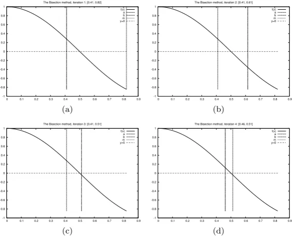
3.6.2 Summarizing Example: Bisection Root Finding . 152 3.7 Exercises . . . 160
4 Array Computing and Curve Plotting . . . 169
4.1 Vectors . . . 170
4.1.1 The Vector Concept . . . 170
4.1.2 Mathematical Operations on Vectors . . . 171
4.1.3 Vector Arithmetics and Vector Functions . . . 173
4.2 Arrays in Python Programs . . . 175
4.2.1 Using Lists for Collecting Function Data . . . 175
4.2.2 Basics of Numerical Python Arrays . . . 176
4.2.3 Computing Coordinates and Function Values . . . 177
4.2.4 Vectorization . . . 178
4.3 Curve Plotting . . . 179
4.3.1 The SciTools and Easyviz Packages . . . 180
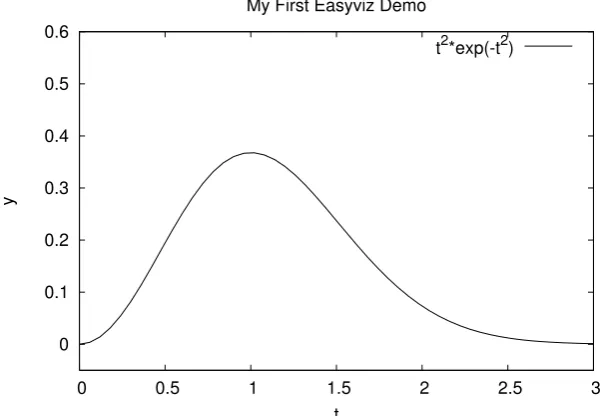
4.3.2 Plotting a Single Curve . . . 181
4.3.3 Decorating the Plot . . . 183
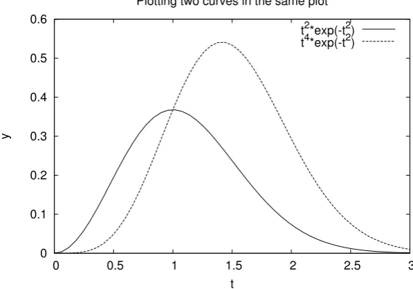
4.3.4 Plotting Multiple Curves . . . 183
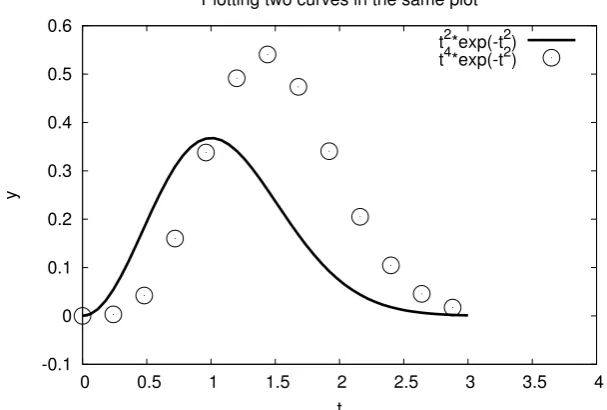
4.3.5 Controlling Line Styles . . . 185
4.3.6 Interactive Plotting Sessions . . . 189
4.3.7 Making Animations . . . 190
4.3.8 Advanced Easyviz Topics . . . 193
4.3.9 Curves in Pure Text . . . 198
4.4 Plotting Difficulties . . . 199
xii Contents
4.4.2 Rapidly Varying Functions . . . 205
4.4.3 Vectorizing StringFunction Objects . . . 206
4.5 More on Numerical Python Arrays . . . 207
4.5.1 Copying Arrays . . . 207
4.5.2 In-Place Arithmetics . . . 207
4.5.3 Allocating Arrays . . . 208
4.5.4 Generalized Indexing . . . 209
4.5.5 Testing for the Array Type . . . 210
4.5.6 Equally Spaced Numbers . . . 211
4.5.7 Compact Syntax for Array Generation . . . 212
4.5.8 Shape Manipulation . . . 212
4.6 Higher-Dimensional Arrays . . . 213
4.6.1 Matrices and Arrays . . . 213
4.6.2 Two-Dimensional Numerical Python Arrays . . . . 214
4.6.3 Array Computing . . . 216
4.6.4 Two-Dimensional Arrays and Functions of Two Variables . . . 217
4.6.5 Matrix Objects . . . 217
4.7 Summary . . . 219
4.7.1 Chapter Topics . . . 219
4.7.2 Summarizing Example: Animating a Function . . 220
4.8 Exercises . . . 225
5 Sequences and Difference Equations . . . 235
5.1 Mathematical Models Based on Difference Equations . . 236
5.1.1 Interest Rates . . . 237
5.1.2 The Factorial as a Difference Equation . . . 239
5.1.3 Fibonacci Numbers . . . 240
5.1.4 Growth of a Population . . . 241
5.1.5 Logistic Growth . . . 242
5.1.6 Payback of a Loan . . . 244
5.1.7 Taylor Series as a Difference Equation . . . 245
5.1.8 Making a Living from a Fortune . . . 246
5.1.9 Newton’s Method . . . 247
5.1.10 The Inverse of a Function . . . 251
5.2 Programming with Sound . . . 253
5.2.1 Writing Sound to File . . . 253
5.2.2 Reading Sound from File . . . 254
5.2.3 Playing Many Notes . . . 255
5.3 Summary . . . 256
5.3.1 Chapter Topics . . . 256
5.3.2 Summarizing Example: Music of a Sequence . . . . 257
5.4 Exercises . . . 260
6.1 Reading Data from File . . . 269
6.1.1 Reading a File Line by Line . . . 270
6.1.2 Reading a Mixture of Text and Numbers . . . 273
6.1.3 What Is a File, Really? . . . 274
6.2 Dictionaries . . . 278
6.2.1 Making Dictionaries . . . 278
6.2.2 Dictionary Operations . . . 279
6.2.3 Example: Polynomials as Dictionaries . . . 280
6.2.4 Example: File Data in Dictionaries . . . 282
6.2.5 Example: File Data in Nested Dictionaries . . . 283
6.2.6 Example: Comparing Stock Prices . . . 287
6.3 Strings . . . 291
6.3.1 Common Operations on Strings . . . 292
6.3.2 Example: Reading Pairs of Numbers . . . 295
6.3.3 Example: Reading Coordinates . . . 298
6.4 Reading Data from Web Pages . . . 300
6.4.1 About Web Pages . . . 300
6.4.2 How to Access Web Pages in Programs . . . 302
6.4.3 Example: Reading Pure Text Files . . . 302
6.4.4 Example: Extracting Data from an HTML Page 304 6.5 Writing Data to File . . . 308
6.5.1 Example: Writing a Table to File . . . 309
6.5.2 Standard Input and Output as File Objects . . . . 310
6.5.3 Reading and Writing Spreadsheet Files . . . 312
6.6 Summary . . . 317
6.6.1 Chapter Topics . . . 317
6.6.2 Summarizing Example: A File Database . . . 319
6.7 Exercises . . . 323
7 Introduction to Classes. . . 337
7.1 Simple Function Classes . . . 338
7.1.1 Problem: Functions with Parameters . . . 338
7.1.2 Representing a Function as a Class . . . 340
7.1.3 Another Function Class Example . . . 346
7.1.4 Alternative Function Class Implementations . . . . 347
7.1.5 Making Classes Without the Class Construct . . . 349
7.2 More Examples on Classes . . . 352
7.2.1 Bank Accounts . . . 352
7.2.2 Phone Book . . . 354
7.2.3 A Circle . . . 355
7.3 Special Methods . . . 356
7.3.1 The Call Special Method . . . 357
7.3.2 Example: Automagic Differentiation . . . 357
7.3.3 Example: Automagic Integration . . . 360
xiv Contents
7.3.5 Example: Phone Book with Special Methods . . . 363
7.3.6 Adding Objects . . . 365
7.3.7 Example: Class for Polynomials . . . 365
7.3.8 Arithmetic Operations and Other Special Methods . . . 369
7.3.9 More on Special Methods for String Conversion . 370 7.4 Example: Solution of Differential Equations . . . 372
7.4.1 A Function for Solving ODEs . . . 373
7.4.2 A Class for Solving ODEs . . . 374
7.4.3 Verifying the Implementation . . . 376
7.4.4 Example: Logistic Growth . . . 377
7.5 Example: Class for Vectors in the Plane . . . 378
7.5.1 Some Mathematical Operations on Vectors . . . 378
7.5.2 Implementation . . . 378
7.5.3 Usage . . . 380
7.6 Example: Class for Complex Numbers . . . 382
7.6.1 Implementation . . . 382
7.6.2 Illegal Operations . . . 383
7.6.3 Mixing Complex and Real Numbers . . . 384
7.6.4 Special Methods for “Right” Operands . . . 387
7.6.5 Inspecting Instances . . . 388
7.7 Static Methods and Attributes . . . 389
7.8 Summary . . . 391
7.8.1 Chapter Topics . . . 391
7.8.2 Summarizing Example: Interval Arithmetics . . . . 392
7.9 Exercises . . . 397
8 Random Numbers and Simple Games . . . 417
8.1 Drawing Random Numbers . . . 418
8.1.1 The Seed . . . 418
8.1.2 Uniformly Distributed Random Numbers . . . 419
8.1.3 Visualizing the Distribution . . . 420
8.1.4 Vectorized Drawing of Random Numbers . . . 421
8.1.5 Computing the Mean and Standard Deviation . . 422
8.1.6 The Gaussian or Normal Distribution . . . 423
8.2 Drawing Integers . . . 424
8.2.1 Random Integer Functions . . . 425
8.2.2 Example: Throwing a Die . . . 426
8.2.3 Drawing a Random Element from a List . . . 427
8.2.4 Example: Drawing Cards from a Deck . . . 427
8.2.5 Example: Class Implementation of a Deck . . . 429
8.3 Computing Probabilities . . . 432
8.3.1 Principles of Monte Carlo Simulation . . . 432
8.3.2 Example: Throwing Dice . . . 433
8.3.4 Example: Policies for Limiting Population
Growth . . . 437
8.4 Simple Games . . . 440
8.4.1 Guessing a Number . . . 440
8.4.2 Rolling Two Dice . . . 440
8.5 Monte Carlo Integration . . . 443
8.5.1 Standard Monte Carlo Integration . . . 443
8.5.2 Computing Areas by Throwing Random Points . 446 8.6 Random Walk in One Space Dimension . . . 447
8.6.1 Basic Implementation . . . 448
8.6.2 Visualization . . . 449
8.6.3 Random Walk as a Difference Equation . . . 449
8.6.4 Computing Statistics of the Particle Positions . . 450
8.6.5 Vectorized Implementation . . . 451
8.7 Random Walk in Two Space Dimensions . . . 453
8.7.1 Basic Implementation . . . 453
8.7.2 Vectorized Implementation . . . 455
8.8 Summary . . . 456
8.8.1 Chapter Topics . . . 456
8.8.2 Summarizing Example: Random Growth . . . 457
8.9 Exercises . . . 463
9 Object-Oriented Programming. . . 479
9.1 Inheritance and Class Hierarchies . . . 479
9.1.1 A Class for Straight Lines . . . 480
9.1.2 A First Try on a Class for Parabolas . . . 481
9.1.3 A Class for Parabolas Using Inheritance . . . 481
9.1.4 Checking the Class Type . . . 483
9.1.5 Attribute versus Inheritance . . . 484
9.1.6 Extending versus Restricting Functionality . . . 485
9.1.7 Superclass for Defining an Interface . . . 486
9.2 Class Hierarchy for Numerical Differentiation . . . 488
9.2.1 Classes for Differentiation . . . 488
9.2.2 A Flexible Main Program . . . 491
9.2.3 Extensions . . . 492
9.2.4 Alternative Implementation via Functions . . . 495
9.2.5 Alternative Implementation via Functional Programming . . . 496
9.2.6 Alternative Implementation via a Single Class . . 497
9.3 Class Hierarchy for Numerical Integration . . . 499
9.3.1 Numerical Integration Methods . . . 499
9.3.2 Classes for Integration . . . 501
9.3.3 Using the Class Hierarchy . . . 504
9.3.4 About Object-Oriented Programming . . . 507
xvi Contents
9.4.1 Mathematical Problem . . . 508 9.4.2 Numerical Methods . . . 510 9.4.3 The ODE Solver Class Hierarchy . . . 511 9.4.4 The Backward Euler Method . . . 515 9.4.5 Verification . . . 518 9.4.6 Application 1:u′=u. . . 518 9.4.7 Application 2: The Logistic Equation . . . 519 9.4.8 Application 3: An Oscillating System . . . 521 9.4.9 Application 4: The Trajectory of a Ball . . . 523 9.5 Class Hierarchy for Geometric Shapes . . . 525 9.5.1 Using the Class Hierarchy . . . 526 9.5.2 Overall Design of the Class Hierarchy . . . 527 9.5.3 The Drawing Tool . . . 529 9.5.4 Implementation of Shape Classes . . . 530 9.5.5 Scaling, Translating, and Rotating a Figure . . . . 534 9.6 Summary . . . 538 9.6.1 Chapter Topics . . . 538 9.6.2 Summarizing Example: Input Data Reader . . . 540 9.7 Exercises . . . 546
B Differential Equations . . . 605 B.1 The Simplest Case . . . 606 B.2 Exponential Growth . . . 608 B.3 Logistic Growth . . . 612 B.4 A General Ordinary Differential Equation . . . 614 B.5 A Simple Pendulum . . . 615 B.6 A Model for the Spread of a Disease . . . 619 B.7 Exercises . . . 621
C A Complete Project. . . 625 C.1 About the Problem: Motion and Forces in Physics . . . 626 C.1.1 The Physical Problem . . . 626 C.1.2 The Computational Algorithm . . . 628 C.1.3 Derivation of the Mathematical Model . . . 628 C.1.4 Derivation of the Algorithm . . . 631 C.2 Program Development and Testing . . . 632 C.2.1 Implementation . . . 632 C.2.2 Callback Functionality . . . 635 C.2.3 Making a Module . . . 636 C.2.4 Verification . . . 637 C.3 Visualization . . . 639 C.3.1 Simultaneous Computation and Plotting . . . 639 C.3.2 Some Applications . . . 642 C.3.3 Remark on Choosing ∆t. . . 643 C.3.4 Comparing Several Quantities in Subplots . . . 644 C.3.5 Comparing Approximate and Exact Solutions . . 645 C.3.6 Evolution of the Error as ∆tDecreases . . . 646 C.4 Exercises . . . 649
D Debugging . . . 651 D.1 Using a Debugger . . . 651 D.2 How to Debug . . . 653 D.2.1 A Recipe for Program Writing and Debugging . . 654 D.2.2 Application of the Recipe . . . 656
xviii Contents
E.5.1 Variable Number of Positional Arguments . . . 679 E.5.2 Variable Number of Keyword Arguments . . . 681 E.6 Evaluating Program Efficiency . . . 683 E.6.1 Making Time Measurements . . . 683 E.6.2 Profiling Python Programs . . . 685
Bibliography. . . 687
List of Exercises
Exercise 1.1 Compute 1+1 . . . 42 Exercise 1.2 Write a “Hello, World!” program . . . 43 Exercise 1.3 Convert from meters to British length units . . . 43 Exercise 1.4 Compute the mass of various substances . . . 43 Exercise 1.5 Compute the growth of money in a bank . . . 43 Exercise 1.6 Find error(s) in a program . . . 43 Exercise 1.7 Type in program text . . . 43 Exercise 1.8 Type in programs and debug them . . . 44 Exercise 1.9 Evaluate a Gaussian function . . . 44 Exercise 1.10 Compute the air resistance on a football . . . 45 Exercise 1.11 Define objects in IPython . . . 45 Exercise 1.12 How to cook the perfect egg . . . 46 Exercise 1.13 Evaluate a function defined by a sum . . . 46 Exercise 1.14 Derive the trajectory of a ball . . . 47 Exercise 1.15 Find errors in the coding of formulas . . . 48 Exercise 1.16 Find errors in Python statements . . . 48 Exercise 1.17 Find errors in the coding of a formula . . . 49 Exercise 2.1 Make a Fahrenheit–Celsius conversion table . . . 99 Exercise 2.2 Generate odd numbers . . . 99 Exercise 2.3 Store odd numbers in a list . . . 100 Exercise 2.4 Generate odd numbers by the range function . . . . 100 Exercise 2.5 Simulate operations on lists by hand . . . 100 Exercise 2.6 Make a table of values from formula (1.1) . . . 100 Exercise 2.7 Store values from formula (1.1) in lists . . . 100 Exercise 2.8 Work with a list . . . 100 Exercise 2.9 Generate equally spaced coordinates . . . 100 Exercise 2.10 Use a list comprehension to solve Exer. 2.9 . . . 101 Exercise 2.11 Store data from Exer. 2.7 in a nested list . . . 101 Exercise 2.12 Compute a mathematical sum . . . 101 Exercise 2.13 Simulate a program by hand . . . 101
xx List of Exercises
Exercise 2.14 Use a for loop in Exer. 2.12 . . . 102 Exercise 2.15 Index a nested lists . . . 102 Exercise 2.16 Construct a double for loop over a nested list . . . . 102 Exercise 2.17 Compute the area of an arbitrary triangle . . . 102 Exercise 2.18 Compute the length of a path . . . 102 Exercise 2.19 Approximatepi. . . 103 Exercise 2.20 Write a Fahrenheit-Celsius conversion table . . . 103 Exercise 2.21 Convert nested list comprehensions to nested
standard loops . . . 103 Exercise 2.22 Write a Fahrenheit–Celsius conversion function . . 104 Exercise 2.23 Write some simple functions . . . 104 Exercise 2.24 Write the program in Exer. 2.12 as a function . . . 104 Exercise 2.25 Implement a Gaussian function . . . 104 Exercise 2.26 Find the max and min values of a function . . . 104 Exercise 2.27 Explore the Python Library Reference . . . 105 Exercise 2.28 Make a function of the formula in Exer. 1.12 . . . . 105 Exercise 2.29 Write a function for numerical differentiation . . . . 105 Exercise 2.30 Write a function for numerical integration . . . 105 Exercise 2.31 Improve the formula in Exer. 2.30 . . . 106 Exercise 2.32 Compute a polynomial via a product . . . 106 Exercise 2.33 Implement the factorial function . . . 106 Exercise 2.34 Compute velocity and acceleration from position
data; one dimension . . . 107 Exercise 2.35 Compute velocity and acceleration from position
data; two dimensions . . . 107 Exercise 2.36 Express a step function as a Python function . . . . 107 Exercise 2.37 Rewrite a mathematical function . . . 108 Exercise 2.38 Make a table for approximations of cosx. . . 108 Exercise 2.39 Implement Exer. 1.13 with a loop . . . 109 Exercise 2.40 Determine the type of objects . . . 109 Exercise 2.41 Implement the sum function . . . 109 Exercise 2.42 Find the max/min elements in a list . . . 110 Exercise 2.43 Demonstrate list functionality . . . 110 Exercise 2.44 Write a sort function for a list of 4-tuples . . . 110 Exercise 2.45 Find prime numbers . . . 111 Exercise 2.46 Condense the program in Exer. 2.14 . . . 111 Exercise 2.47 Values of boolean expressions . . . 112 Exercise 2.48 Explore round-off errors from a large number of
Exercise 2.55 Explore problems with inaccurate indentation . . . 115 Exercise 2.56 Find an error in a program . . . 115 Exercise 2.57 Find programming errors . . . 116 Exercise 2.58 Simulate nested loops by hand . . . 117 Exercise 2.59 Explore punctuation in Python programs . . . 117 Exercise 2.60 Investigate a for loop over a changing list . . . 117 Exercise 3.1 Make an interactive program . . . 160 Exercise 3.2 Read from the command line in Exer. 3.1 . . . 160 Exercise 3.3 Use exceptions in Exer. 3.2 . . . 160 Exercise 3.4 Read input from the keyboard . . . 161 Exercise 3.5 Read input from the command line . . . 161 Exercise 3.6 Prompt the user for input to the formula (1.1) . . . 161 Exercise 3.7 Read command line input for the formula (1.1) . . 161 Exercise 3.8 Make the program from Exer. 3.7 safer . . . 161 Exercise 3.9 Test more in the program from Exer. 3.7 . . . 161 Exercise 3.10 Raise an exception in Exer. 3.9 . . . 161 Exercise 3.11 Look up calendar functionality . . . 162 Exercise 3.12 Use the StringFunction tool . . . 162 Exercise 3.13 Extend a program from Ch. 3.2.1 . . . 162 Exercise 3.14 Why we test for specific exception types . . . 162 Exercise 3.15 Make a simple module . . . 163 Exercise 3.16 Make a useful main program for Exer. 3.15 . . . 163 Exercise 3.17 Make a module in Exer. 2.39 . . . 163 Exercise 3.18 Extend the module from Exer. 3.17 . . . 163 Exercise 3.19 Use options and values in Exer. 3.18 . . . 163 Exercise 3.20 Use optparse in the program from Ch. 3.2.4 . . . 163 Exercise 3.21 Compute the distance it takes to stop a car . . . 163 Exercise 3.22 Check if mathematical rules hold on a computer . 164 Exercise 3.23 Improve input to the program in Exer. 3.22 . . . 164 Exercise 3.24 Apply the program from Exer. 3.23 . . . 165 Exercise 3.25 Compute the binomial distribution . . . 165 Exercise 3.26 Apply the binomial distribution . . . 166 Exercise 3.27 Compute probabilities with the Poisson
distribution . . . 166 Exercise 4.1 Fill lists with function values . . . 225 Exercise 4.2 Fill arrays; loop version . . . 226 Exercise 4.3 Fill arrays; vectorized version . . . 226 Exercise 4.4 Apply a function to a vector . . . 226 Exercise 4.5 Simulate by hand a vectorized expression . . . 226 Exercise 4.6 Demonstrate array slicing . . . 227 Exercise 4.7 Plot the formula (1.1) . . . 227 Exercise 4.8 Plot the formula (1.1) for several v0 values . . . 227
Exercise 4.9 Plot exact and inexact Fahrenheit–Celsius
xxii List of Exercises
xxiv List of Exercises
xxvi List of Exercises
Exercise 9.15 Compute convergence rates of numerical
integration methods . . . 550 Exercise 9.16 Add common functionality in a class hierarchy . . 551 Exercise 9.17 Make a class hierarchy for root finding . . . 552 Exercise 9.18 Use the ODESolver hierarchy to solve a simple
Computing with Formulas
1
Our first examples on computer programming involve programs that evaluate mathematical formulas. You will learn how to write and run a Python program, how to work with variables, how to compute with mathematical functions such as ex and sinx, and how to use Python for interactive calculations.
We assume that you are somewhat familiar with computers so that you know what files and folders1
are, how you move between folders, how you change file and folder names, and how you write text and save it in a file.
All the program examples associated with this chapter can be found as files in the folder src/formulas. We refer to the preface for how to download the folder tree src containing all the program files for this book.
1.1 The First Programming Encounter: A Formula
The first formula we shall consider concerns the vertical motion of a ball thrown up in the air. From Newton’s second law of motion one can set up a mathematical model for the motion of the ball and find that the vertical position of the ball, called y, varies with time taccording to the following formula2
:
y(t) =v0t−
1 2gt
2. (1.1)
1 Another frequent word for folder is directory.
2 This formula neglects air resistance, which is usually small unless
v0 is large – see
Exercise 1.10.
Here,v0is the initial velocity of the ball,gis the acceleration of gravity,
andtis time. Observe that theyaxis is chosen such that the ball starts aty= 0 when t= 0.
To get an overview of the time it takes for the ball to move upwards and return to y = 0 again, we can look for solutions to the equation
y= 0:
v0t−
1 2gt
2 =t(v 0−
1
2gt) = 0 : t= 0 or t= 2v0/g .
That is, the ball returns after 2v0/g seconds, and it is therefore
rea-sonable to restrict the interest of (1.1) tot∈[0,2v0/g].
1.1.1 Using a Program as a Calculator
Our first program will evaluate (1.1) for a specific choice ofv0,g, and
t. Choosingv0 = 5m/s and g = 9.81 m/s2 makes the ball come back
after t = 2v0/g ≈ 1 s. This means that we are basically interested in
the time interval [0,1]. Say we want to compute the height of the ball at timet= 0.6s. From (1.1) we have
y= 5·0.6−1
2·9.81·0.6
2
This arithmetic expression can be evaluated and its value can be printed by a very simple one-line Python program:
print 5*0.6 - 0.5*9.81*0.6**2
The four standard arithmetic operators are written as +,-, *, and
/in Python and most other computer languages. The exponentiation employs a double asterisk notation in Python, e.g., 0.62 is written as
0.6**2.
Our task now is to create the program and run it, and this will be described next.
1.1.2 About Programs and Programming
1.1 The First Programming Encounter: A Formula 3
Another perception of the word “program” is a file that can be run (“double-clicked”) to perform a task. Sometimes this is a file with tex-tual instructions (which is the case with Python), and sometimes this file is a translation of all the program text to a more efficient and computer-friendly language that is quite difficult to read for a human. All the programs in this chapter consist of short text stored in a single file. Other programs that you have used frequently, for instance Fire-fox or Internet Explorer for reading web pages, consist of program text distributed over a large number of files, written by a large number of people over many years. One single file contains the machine-efficient translation of the whole program, and this is normally the file that you “double-click” on when starting the program. In general, the word “program” means either this single file or the collection of files with
textual instructions.
Programming is obviously about writing programs, but this process is more than writing the correct instructions in a file. First, we must understand how a problem can be solved by giving a sequence of in-structions to the computer. This is usually the most difficult thing with programming. Second, we must express this sequence of instructions correctly in a computer language and store the corresponding text in a file (the program). Third, we must run the program, check the validity of the results, and usually enter a fourth phase where errors in the pro-gram must be found and corrected. Mastering this process requires a lot of training, which implies making a large number of programs (ex-ercises in this book, for instance) and getting the programs to work.
1.1.3 Tools for Writing Programs
Since programs consist of plain text, we need to write this text with the help of another program that can store the text in a file. You have most likely extensive experience with writing text on a computer, but for writing your own programs you need special programs, callededitors, which preserve exactly the characters you type. The widespread word processors, Microsoft Word being a primary example3
, are aimed at producing nice-looking reports. These programs format the text and arenotgood tools for writing your own programs, even though they can save the document in a pure text format. Spaces are often important in Python programs, andeditors for plain text give you complete control of the spaces and all other characters in the program file.
3 Other examples are OpenOffice, TextEdit, iWork Pages, and BBEdit. Chapter 6.1.3
Emacs, XEmacs, and Vim are popular editors for writing programs on Linux or Unix systems, including Mac4
computers. On Windows we recommend Notepad++ or the Window versions of Emacs or Vim. None of these programs are part of a standard Windows installation.
A special editor for Python programs comes with the Python soft-ware. This editor is called Idle and is usually installed under the name
idle (or idle-python) on Linux/Unix and Mac. On Windows, it is
reachable from the Python entry in the Start menu. Idle has a gentle learning curve, but is mainly restricted to writing Python programs. Completely general editors, such as Emacs and Vim, have a steeper learning curve and can be used for any text files, including reports in student projects.
1.1.4 Using Idle to Write the Program
Let us explain in detail how we can use Idle to write our one-line program from Chapter 1.1.1. Idle may not become your favorite editor for writing Python programs, yet we recommend to follow the steps below to get in touch with Idle and try it out. You can simply replace the Idle instructions by similar actions in your favorite editor, Emacs for instance.
First, create a folder where your Python programs can be located. Here we choose a folder name py1st under your home folder (note that the third character is the number 1, not the letter l – the name reflects your 1st try of Python). To write and run Python programs, you will need a terminal window on Linux/Unix or Mac, sometimes called a console window, or a DOS window on Windows. Launch such a window and use thecd (change directory) command to move to the
py1st folder. If you have not made the folder with a graphical file
& folder manager you must create the folder by the command mkdir
py1st(mkdirstands for make directory).
The next step is to start Idle. This can be done by writing idle&
(Linux) or start idle (Windows) in the terminal window. Alterna-tively, you can launch Idle from the Start menu on Windows. Fig-ure 1.1 displays a terminal window where we create the folder, move to the folder, and start Idle5
.
If a window now appears on the screen, with “Python Shell” in the title bar of the window, go to its File menu and choose New Window.
4 On Mac, you may want to download a more “Mac-like” editor such as the Really
Simple Text program.
5 The ampersand after
1.1 The First Programming Encounter: A Formula 5
Fig. 1.1 A terminal window on a Linux/Unix/Mac machine where we create a folder (mkdir), move to the folder (cd), and start Idle.
The window that now pops up is the Idle editor (having the window name “Untitled”). Move the cursor inside this window and write the line
print 5*0.6 - 0.5*9.81*0.6**2
followed by pressing the Return key. The Idle window looks as in Fig-ure 1.2.
Fig. 1.2 An Idle editor window containing our first one-line program.
is no need to navigate and change folder. Simply fill in the name of the program. Any name will do, but we suggest that you choose the
name ball_numbers.pybecause this name is compatible with what we
use later in this book. The file extension .py is common for Python programs, but not strictly required6
.
Press the Save button and move back to the terminal window. Make sure you have a new file ball_numbers.py here, by running the com-mandls(on Linux/Unix and Mac) ordir(on Windows). The output should be a text containing the name of the program file. You can now jump to the paragraph “How to Run the Program”, but it might be a good idea to read the warning below first.
Warning About Typing Program Text. Even though a program is just a text, there is one major difference between a text in a program and a text intended to be read by a human. When a human reads a text, she or he is able to understand the message of the text even if the text is not perfectly precise or if there are grammar errors. If our one-line program was expressed as
write 5*0.6 - 0.5*9.81*0.6^2
most humans would interpretwriteand print as the same thing, and many would also interpret6^2as 62. In the Python language, however,
write is a grammar error and 6^2 means an operation very different
from the exponentiation 6**2. Our communication with a computer through a program must be perfectly precise without a single grammar error7
. The computer will only do exactly what we tell it to do. Any error in the program, however small, may affect the program. There is a chance that we will never notice it, but most often an error causes the program to stop or produce wrong results. The conclusion is that computers have a much more pedantic attitude to language than what (most) humans have.
Now you understand why any program text must be carefully typed, paying attention to the correctness of every character. If you try out program texts from this book, make sure that you type them inexactly as you see them in the book. Blanks, for instance, are often important in Python, so it is a good habit to always count them and type them in correctly. Any attempt not to follow this advice will cause you frus-trations, sweat, and maybe even tears.
6 Some editors, like Emacs, have many features that make it easier to write Python
programs, but these features will not be automatically available unless the program file has a.pyextension.
7“Programming demands significantly higher standard of accuracy. Things don’t
1.1 The First Programming Encounter: A Formula 7
1.1.5 How to Run the Program
The one-line program above is stored in a file with name
ball_numbers.py. To run the program, you need to be in a
termi-nal window and in the folder where the ball_numbers.py file resides. The program is run by writing the commandpython ball_numbers.py
in the terminal window8
:
Terminal
Unix/DOS> python ball_numbers.py 1.2342
The program immediately responds with printing the result of its calcu-lation, and the output appears on the next line in the terminal window. In this book we use the promptUnix/DOS>to indicate a command line in a Linux, Unix, Mac, or DOS terminal window (a command line means that we can run Unix or DOS commands, such ascd andpython). On your machine, you will likely see a different prompt. Figure 1.3 shows what the whole terminal window may look like after having run the program.
Fig. 1.3 A terminal window on a Linux/Unix/Mac machine where we run our first one-line Python program.
From your previous experience with computers you are probably used to double-click on icons to run programs. Python programs can also be run that way, but programmers usually find it more convenient to run programs by typing commands in a terminal window. Why this is so will be evident later when you have more programming experience. For now, simply accept that you are going to be a programmer, and that commands in a terminal window is an efficient way to work with the computer.
Suppose you want to evaluate (1.1) for v0 = 1 and t= 0.1. This is
easy: move the cursor to the Idle editor window, edit the program text to
print 1*0.1 - 0.5*9.81*0.1**2
Save the file, move back to the terminal window and run the program as before:
Terminal
Unix/DOS> python ball_numbers.py 0.05095
We see that the result of the calculation has changed, as expected.
1.1.6 Verifying the Result
We shouldalways carefully control that the output of a computer pro-gram is correct. You will experience that in most of the cases, at least until you are an experienced programmer, the output is wrong, and you have to search for errors. In the present application we can simply use a calculator to control the program. Setting t= 0.6and v0 = 5 in
the formula, the calculator confirms that 1.2342 is the correct solution to our mathematical problem.
1.1.7 Using Variables
When we want to evaluatey(t)for many values oft, we must modify the
tvalue at two places in our program. Changing another parameter, like
v0, is in principle straightforward, but in practice it is easy to modify
the wrong number. Such modifications would be simpler to perform if we express our formula in terms of variables, i.e., symbols, rather than numerical values. Most programming languages, Python included, have variables similar to the concept of variables in mathematics. This means that we can define v0,g,t, and y as variables in the program, initialize the former three with numerical values, and combine these three variables to the desired right-hand side expression in (1.1), and assign the result to the variabley.
The alternative version of our program, where we use variables, may be written as this text:
v0 = 5 g = 9.81 t = 0.6
y = v0*t - 0.5*g*t**2 print y
Figure 1.4 displays what the program looks like in the Idle editor win-dow. Variables in Python are defined by setting a name (here v0, g,
1.1 The First Programming Encounter: A Formula 9
Fig. 1.4 An Idle editor window containing a multi-line program with several variables.
Note that this second program is much easier to read because it is closer to the mathematical notation used in the formula (1.1). The pro-gram is also safer to modify, because we clearly see what each number is when there is a name associated with it. In particular, we can change
t at one place only (the linet = 0.6) and not two as was required in the previous program.
We store the program text in a fileball_variables.py. Running the program,
Terminal
Unix/DOS> python ball_variables.py
results in the correct output1.2342.
1.1.8 Names of Variables
Introducing variables with descriptive names, close to those in the mathematical problem we are going to solve, is considered important for the readability and reliability (correctness) of the program. Vari-able names can contain any lower or upper case letter, the numbers from 0 to 9, and underscore, but the first character cannot be a num-ber. Python distinguishes between upper and lower case, soXis always different fromx. Here are a few examples on alternative variable names in the present example9
:
initial_velocity = 5
acceleration_of_gravity = 9.81 TIME = 0.6
VerticalPositionOfBall = initial_velocity*TIME - \
0.5*acceleration_of_gravity*TIME**2 print VerticalPositionOfBall
9 In this book we shall adopt the rule that variable names have lower case letters
With such long variables names, the code for evaluating the formula becomes so long that we have decided to break it into two lines. This is done by a backslash at the very end of the line (make sure there are no blanks after the backslash!).
We note that even if this latter version of the program contains variables that are defined precisely by their names, the program is harder to read than the one with variablesv0,g,t, andy0.
The rule of thumb is to use the same variable names as those ap-pearing in a precise mathematical description of the problem to be solved by the program. For all variables where there is no associated precise mathematical description and symbol, one must usedescriptive
variable names which explain the purpose of the variable. For example, if a problem description introduces the symbolDfor a force due to air resistance, one applies a variableDalso in the program. However, if the problem description does not define any symbol for this force, one must apply a descriptive name, such as air_resistance, resistance_force,
ordrag_force.
1.1.9 Reserved Words in Python
Certain words are reserved in Python because they are used to build up the Python language. These reserved words cannot be used as variable names: and, as, assert, break, class, continue, def, del, elif, else,
except, False, finally, for, from, global, if, import, in, is, lambda,
None,nonlocal,not,or,pass,raise,return,True,try,with,while, and
yield. You may, for instance, add an underscore at the end to turn a
reserved word into a variable name. See Exercise 1.16 for examples on legal and illegal variable names.
1.1.10 Comments
Along with the program statements it is often informative to provide some comments in a natural human language to explain the idea behind the statements. Comments in Python start with the # character, and everything after this character on a line is ignored when the program is run. Here is an example of our program with explanatory comments:
# program for computing the height of a ball thrown up in the air v0 = 5 # initial velocity
g = 9.81 # acceleration of gravity t = 0.6 # time
y = v0*t - 0.5*g*t**2 # vertical position print y
1.1 The First Programming Encounter: A Formula 11
Good comments together with well-chosen variable names are nec-essary for any program longer than a few lines, because otherwise the program becomes difficult to understand, both for the programmer and others. It requires some practice to write really instructive comments. Never repeat with words what the program statements already clearly express. Use instead comments to provide important information that is not obvious from the code, for example, what mathematical variable names mean, what variables are used for, and general ideas that lie behind a forthcoming set of statements.
1.1.11 Formatting Text and Numbers
Instead of just printing the numerical value of y in our introductory program, we now want to write a more informative text, typically some-thing like
At t=0.6 s, the height of the ball is 1.23 m.
where we also have control of the number of digits (here y is accurate up to centimeters only).
Such output from the program is accomplished by a print state-ment where we use something often known as printf formatting10
. For a newcomer to programming, the syntax of printf formatting may look awkward, but it is quite easy to learn and very convenient and flexible to work with. The sample output above is produced by this statement:
print ’At t=%g s, the height of the ball is %.2f m.’ % (t, y)
Let us explain this line in detail. The print statement now prints a string: everything that is enclosed in quotes (either single: ’, or
dou-ble:") denotes a string in Python. The string above is formatted using
printf syntax. This means that the string has various “slots”, start-ing with a percentage sign, here %g and %.2f, where variables in the program can be put in. We have two “slots” in the present case, and consequently two variables must be put into the slots. The relevant syntax is to list the variables inside standard parentheses after the string, separated from the string by a percentage sign. The first vari-able,t, goes into the first “slot”. This “slot” has a format specification
%g, where the percentage sign marks the slot and the following char-acter, g, is a format specification. The g that a real number is to be written as compactly as possible. The next variable, y, goes into the second “slot”. The format specification here is.2f, which means a real number written with two digits after comma. Thefin the .2fformat
10This formatting was originally introduced by a functionprintfin the C
stands for float, a short form for floating-point number, which is the term used for a real number on a computer.
For completeness we present the whole program, where text and numbers are mixed in the output:
v0 = 5 g = 9.81 t = 0.6
y = v0*t - 0.5*g*t**2
print ’At t=%g s, the height of the ball is %.2f m.’ % (t, y)
You can find the program in the file ball_output1.py in the
src/formulasfolder.
There are many more ways to specify formats. For example,ewrites a number inscientific notation, i.e., with a number between 1 and 10 followed by a power of 10, as in 1.2432·10−3. On a computer such a
number is written in the form 1.2432e-03. Capital E in the exponent is also possible, just replace eby E, with the result1.2432E-03.
For decimal notation we use the letter f, as in %f, and the output number then appears with digits before and/or after a comma, e.g.,
0.0012432 instead of 1.2432E-03. With the g format, the output will
use scientific notation for large or small numbers and decimal notation otherwise. This format is normally what gives most compact output of a real number. A lower casegleads to lower caseein scientific notation, while upper caseG impliesE instead of e in the exponent.
One can also specify the format as10.4f or 14.6E, meaning in the first case that a float is written in decimal notation with four decimals in a field of width equal to 10 characters, and in the second case a float written in scientific notation with six decimals in a field of width 14 characters.
Here is a list of some important printf format specifications11
:
%s a string
%d an integer
%0xd an integer padded with x leading zeros %f decimal notation with six decimals
%e compact scientific notation, e in the exponent %E compact scientific notation, E in the exponent %g compact decimal or scientific notation (with e) %G compact decimal or scientific notation (with E) %xz format z right-adjusted in a field of width x %-xz format z left-adjusted in a field of width x %.yz format z with y decimals
%x.yz format z with y decimals in a field of width x %% the percentage sign (%) itself
The programprintf_demo.pyexemplifies many of these formats. We may try out some formats by writing more numbers to the screen in our program (the corresponding file isball_output2.py):
11For a complete specification of the possible printf-style format strings, follow the
1.2 Computer Science Glossary 13
v0 = 5 g = 9.81 t = 0.6
y = v0*t - 0.5*g*t**2 print """
At t=%f s, a ball with initial velocity v0=%.3E m/s is located at the height %.2f m. """ % (t, v0, y)
Observe here that we use atriple-quoted string, recognized by starting and ending with three single or double quotes: ’or""". Triple-quoted strings are used for text that spans several lines.
In the print statement above, we write t in the f format, which by default implies six decimals;v0 is written in the.3Eformat, which implies three decimals and the number spans as narrow field as possible; and y is written with two decimals in decimal notation in as narrow field as possible. The output becomes
Terminal
Unix/DOS> python ball_fmt2.py
At t=0.600000 s, a ball with initial velocity v0=5.000E+00 m/s is located at the height 1.23 m.
You should look at each number in the output and check the formatting in detail.
The Newline Character. We often want a computer program to write out text that spans several lines. In the last example we obtained such output by triple-quoted strings. We could also use ordinary single-quoted strings and a special character for indicating where line breaks should occur. This special character reads\n, i.e., a backslash followed by the letter n. The two printstatements
print """y(t) is the position of our ball."""
print ’y(t) is\nthe position of\nour ball’
result in identical output:
y(t) is
the position of our ball.
1.2 Computer Science Glossary
debug, debugging, execute, executable, implement, implementation, in-put, library, operating system, outin-put, statement, syntax, user, verify, and verification.
These words are frequently used in English in lots of contexts, yet they have a precise meaning in computer science.
Program and code are interchangeable terms. A code/program seg-mentis a collection of consecutive statements from a program. Another term with similar meaning iscode snippet. Many also use the word ap-plication in the same meaning as program and code. A related term is
source code, which is the same as the text that constitutes the program. You find the source code of a program in one or more text files12
. We talk about running a program, or equivalently executing a pro-gram or executing a file. The file we execute is the file in which the program text is stored. This file is often called an executable or an
application. The program text may appear in many files, but the ex-ecutable is just the single file that starts the whole program when we run that file. Running a file can be done in several ways, for instance, by double-clicking the file icon, by writing the filename in a terminal window, or by giving the filename to some program. This latter tech-nique is what we have used so far in this book: we feed the filename to the programpython. That is, we execute a Python program by execut-ing another program python, which interprets the text in our Python program file.
The term library is widely used for a collection of generally useful program pieces that can be applied in many different contexts. Hav-ing access to good libraries means that you do not need to program code snippets that others have already programmed (most probable in a better way!). There are huge numbers of Python libraries. In Python terminology, the libraries are composed ofmodules and pack-ages. Chapter 1.4 gives a first glimpse of the math module, which con-tains a set of standard mathematical functions for sinx, cosx, lnx,ex, sinhx, sin−1x, etc. Later, you will meet many other useful modules.
Packages are just collections of modules. The standard Python dis-tribution comes with a large number of modules and packages, but you can download many more from the Internet, see in particular
www.python.org/pypi. Very often, when you encounter a programming
task that is likely to occur in many other contexts, you can find a Python module where the job is already done. To mention just one example, say you need to compute how many days there are between two dates. This is a non-trivial task that lots of other programmers must have faced, so it is not a big surprise that Python comes with a module datetimeto do calculations with dates.
12Note that text files normally have the extension.txt, while program files have an
![Fig. 2.1Illustration of two variables:21, 29, 4.0]var2 = [20, 21, 29, 4.0] var1 refers to an int object with value 21,created by the statement var1 = 21, and var2 refers to a list object with value [20,, i.e., three int objects and one float object, created by the statement.](https://thumb-us.123doks.com/thumbv2/123dok_us/1488015.688864/89.547.279.373.318.415/illustration-variables-created-statement-refers-objects-created-statement.webp)
![Figure 3.2 displays graphically the first four steps of this algorithmfor solving the equation[0 cos(πx) = 0, starting with the interval, 0.82]](https://thumb-us.123doks.com/thumbv2/123dok_us/1488015.688864/186.547.57.243.480.606/figure-displays-graphically-algorithmfor-solving-equation-starting-interval.webp)