Obstacle avoidance &motion planning by stochastic processes, spatial description, sensor integration and trajectory generation in the domain of embedded systems, mechatronics, artificial intelligence, robotics and machine learning

OBSTACLE AVOIDANCE &MOTION PLANNING BY STOCHASTIC PROCESSES, SPATIAL

DESCRIPTION, SENSOR INTEGRATION AND TRAJECTORY GENERATION IN THE

DOMAIN OF EMBEDDED SYSTEMS, MECHATRONICS, ARTIFICIAL

INTELLIGENCE, ROBOTICS AND MACHINE LEARNING

*,1

_{Pavleen S Bali,}

_{Prof. (Dr.) A K Raghav,}

_{Ankur Siwach,}

_{Yash Narula,}

1

_{Research Associate, E & C Engg. Dept., Amity University Haryana, Gurgaon 122 413, India}

2

_{Director, Industrial R&D, Amity University Haryana, Gurgaon 122413, India}

3

_{Asst. Professor, E & C Engg. Dept., Amity University Haryana, Gurgaon 122 413, India}

4

_{Mechanical Engg. Dept., Amity University Haryana, Gurgaon 122 413, India}

5

_{Computer Science Engg. Dept., MRKIE}

ARTICLE INFO ABSTRACT

In this paper, we describe a representation for spatial information, called the stochastic map, and associated procedures for building it, reading information from it, and revising it incrementally as new information is obtained. The ma

all the available information. The procedures provide a general solution to the problem of estimating uncertain relative spatial relationships and trajectory

the previous, very conservative, worst context of state

Traditionally, the dynamic model, i.e., the equations of motion, of a robotic system is derived from Euler Lagrange (EL) or Newton

generalized coordinates, whereas the NE equations are based on the Cartesian coordinates. The NE equations consider various forces and moments on the free body diagram of each link of the robotic system at hand, and, hence, require the calculation of the constrai

motion of the coupled system. Hence, the principle of elimination of constraint forces has been proposed in the literature. One such methodology is based on the Decoupled Natural Orthogonal C

reported elsewhere. It is shown in this paper that one can also begin with the EL equations of motion based on the kinetic and potential energies of the system, and use the DeNOC matrices to obtain the independent equations of motion. The advantage of the proposed approach is that a computationally more efficient forward dynamics algorithm for the serial robots having slender rods is obtained, which is numerically stable. The typical six of-freedom PUMA robot is considered

obstacle avoidance, motion planning and dynamic simulation comes in the trajectory generation part. Spatial description and trajectory generation work simultaneously for the proper func

trajectory generation is in common usage in robotics to provide smooth, continuous motion from one set of n joint angles to another, for instance for moving between two distinct Cartesian poses for which the inverse pose has yielded two distinct sets of n joint angles. The joint

joints independently but simultaneously.

Copyright © 2016, Pavleen S Bali et al. This is an open access article distributed under use, distribution, and reproduction in any medium, provided the original work is properly cited.

INTRODUCTION

In many applications of robotics, such as industrial automation, and autonomous mobility, there is a need to represent and reason about spatial uncertainty. In the past, this need has been

*Corresponding author: Pavleen S Bali,

Research Associate, E & C Engg. Dept., Amity University Haryana, Gurgaon 122 413, India.

ISSN: 0975-833X

Article History: Received 23rd January, 2016 Received in revised form 26th _{February, 2016}

Accepted 09th _{March, 2016}

Published online 26th _April,2016

Key words: Stochastic Process, Spatial Description, Frame Transformation, Inverse Kinematics, Forward Kinematics, Trajectory Generation, Obstacle Avoidance, Motion Planning, R Matrix, DH Parameters, D Cosines etc.

Citation: Pavleen S Bali, Prof. (Dr.) A K Raghav, Manoj Pandey

description, sensor integration and trajectory generation in the domain of embedded systems, mechatronics, artificial intelli learning”, International Journal of Current Research, 8, (04),

RESEARCH ARTICLE

MOTION PLANNING BY STOCHASTIC PROCESSES, SPATIAL

DESCRIPTION, SENSOR INTEGRATION AND TRAJECTORY GENERATION IN THE

DOMAIN OF EMBEDDED SYSTEMS, MECHATRONICS, ARTIFICIAL

INTELLIGENCE, ROBOTICS AND MACHINE LEARNING

Prof. (Dr.) A K Raghav,

_{Manoj Pandey,}

_{Shuvam Gupta,}

Yash Narula,

_{Rahul Verma,}

_{Deepak Jataywal and}

Research Associate, E & C Engg. Dept., Amity University Haryana, Gurgaon 122 413, India

trial R&D, Amity University Haryana, Gurgaon 122413, India

Asst. Professor, E & C Engg. Dept., Amity University Haryana, Gurgaon 122 413, India

Mechanical Engg. Dept., Amity University Haryana, Gurgaon 122 413, India

Computer Science Engg. Dept., MRKIET, Rewari 123401, Haryana, India

In this paper, we describe a representation for spatial information, called the stochastic map, and associated procedures for building it, reading information from it, and revising it incrementally as new information is obtained. The map contains the estimates of relationships among objects in the map, and their uncertainties, given all the available information. The procedures provide a general solution to the problem of estimating uncertain relative spatial relationships and trajectory description. The estimates are probabilistic in nature, an advance over the previous, very conservative, worst-case approaches to the problem. Finally, the procedures are developed in the context of state-estimation and filtering theory, which provides a

Traditionally, the dynamic model, i.e., the equations of motion, of a robotic system is derived from Euler Lagrange (EL) or Newton–Euler (NE) equations. The EL equations begin with a set of generally independent

ized coordinates, whereas the NE equations are based on the Cartesian coordinates. The NE equations consider various forces and moments on the free body diagram of each link of the robotic system at hand, and, hence, require the calculation of the constrained forces and moments that eventually do not participate in the motion of the coupled system. Hence, the principle of elimination of constraint forces has been proposed in the literature. One such methodology is based on the Decoupled Natural Orthogonal C

reported elsewhere. It is shown in this paper that one can also begin with the EL equations of motion based on the kinetic and potential energies of the system, and use the DeNOC matrices to obtain the independent equations of otion. The advantage of the proposed approach is that a computationally more efficient forward dynamics algorithm for the serial robots having slender rods is obtained, which is numerically stable. The typical six

freedom PUMA robot is considered here to illustrate the advantages of the proposed algorithm. Moreover obstacle avoidance, motion planning and dynamic simulation comes in the trajectory generation part. Spatial description and trajectory generation work simultaneously for the proper func

trajectory generation is in common usage in robotics to provide smooth, continuous motion from one set of n joint angles to another, for instance for moving between two distinct Cartesian poses for which the inverse pose has yielded two distinct sets of n joint angles. The joint-space trajectory generation occurs at runtime for all n joints independently but simultaneously.

is an open access article distributed under the Creative Commons Attribution License, which use, distribution, and reproduction in any medium, provided the original work is properly cited.

In many applications of robotics, such as industrial automation, and autonomous mobility, there is a need to represent and reason about spatial uncertainty. In the past, this need has been

Engg. Dept., Amity University Haryana, Gurgaon

circumvented by special purpose methods such as precision engineering, very accurate sensors and the use of fixtures and calibration points. While these methods sometimes supply sufficient accuracy to avoid the need to represent uncertainty explicitly, they are usually costly. An alternative approach is to use multiple, overlapping, lower resolution sensors and to combine the spatial information (including the uncertainty) from all sources to obtain the best spatial estimate.

Available online at http://www.journalcra.com

International Journal of Current Research

Vol. 8, Issue, 04, pp.29360-29371, April, 2016

INTERNATIONAL

Pavleen S Bali, Prof. (Dr.) A K Raghav, Manoj Pandey et al. 2016. “Obstacle avoidance &motion planning by stochastic processes, spatial description, sensor integration and trajectory generation in the domain of embedded systems, mechatronics, artificial intelli

, 8, (04), 29360-29371.

z

MOTION PLANNING BY STOCHASTIC PROCESSES, SPATIAL

DESCRIPTION, SENSOR INTEGRATION AND TRAJECTORY GENERATION IN THE

DOMAIN OF EMBEDDED SYSTEMS, MECHATRONICS, ARTIFICIAL

INTELLIGENCE, ROBOTICS AND MACHINE LEARNING

Shuvam Gupta,

_{Harivansh, K.,}

Deepak Jataywal and

_{Sandeep Singh}

Research Associate, E & C Engg. Dept., Amity University Haryana, Gurgaon 122 413, India

trial R&D, Amity University Haryana, Gurgaon 122413, India

Asst. Professor, E & C Engg. Dept., Amity University Haryana, Gurgaon 122 413, India

Mechanical Engg. Dept., Amity University Haryana, Gurgaon 122 413, India

T, Rewari 123401, Haryana, India

In this paper, we describe a representation for spatial information, called the stochastic map, and associated procedures for building it, reading information from it, and revising it incrementally as new information is p contains the estimates of relationships among objects in the map, and their uncertainties, given all the available information. The procedures provide a general solution to the problem of estimating uncertain description. The estimates are probabilistic in nature, an advance over case approaches to the problem. Finally, the procedures are developed in the estimation and filtering theory, which provides a solid basis for numerous extensions. Traditionally, the dynamic model, i.e., the equations of motion, of a robotic system is derived from Euler–

Euler (NE) equations. The EL equations begin with a set of generally independent ized coordinates, whereas the NE equations are based on the Cartesian coordinates. The NE equations consider various forces and moments on the free body diagram of each link of the robotic system at hand, and, ned forces and moments that eventually do not participate in the motion of the coupled system. Hence, the principle of elimination of constraint forces has been proposed in the literature. One such methodology is based on the Decoupled Natural Orthogonal Complement (DeNOC) matrices, reported elsewhere. It is shown in this paper that one can also begin with the EL equations of motion based on the kinetic and potential energies of the system, and use the DeNOC matrices to obtain the independent equations of otion. The advantage of the proposed approach is that a computationally more efficient forward dynamics algorithm for the serial robots having slender rods is obtained, which is numerically stable. The typical

six-degree-here to illustrate the advantages of the proposed algorithm. Moreover obstacle avoidance, motion planning and dynamic simulation comes in the trajectory generation part. Spatial description and trajectory generation work simultaneously for the proper functioning of the robot. Joint-space trajectory generation is in common usage in robotics to provide smooth, continuous motion from one set of n joint angles to another, for instance for moving between two distinct Cartesian poses for which the inverse pose solution space trajectory generation occurs at runtime for all n

ribution License, which permits unrestricted

circumvented by special purpose methods such as precision engineering, very accurate sensors and the use of fixtures and calibration points. While these methods sometimes supply sufficient accuracy to avoid the need to represent uncertainty y are usually costly. An alternative approach is to use multiple, overlapping, lower resolution sensors and to combine the spatial information (including the uncertainty) from all sources to obtain the best spatial estimate.

INTERNATIONAL JOURNAL OF CURRENT RESEARCH

Fig 1. Configuration Parameters

This integrated information can often supply sufficient accuracy to avoid the need for the hard engineered approach. In addition to lower hardware cost, the explicit estimation of uncertain spatial information makes it possible to decide in advance whether proposed operations are likely to fail because of accumulated uncertainty, and whether proposed sensor information will be sufficient to reduce the uncertainty to tolerable limits. In situations utilizing inexpensive mobile robots, perhaps the only way to obtain sufficient accuracy is to combine the (uncertain information from many sensors. However, a difficulty in combining uncertain spatial information arises because it often occurs in the form of uncertain relative information. This is particularly true where many different frames of reference are used, and the uncertain spatial information must be propagated between these frames. This paper presents a general solution to the problem of estimating uncertain spatial relationships, regardless of which frame the information is presented in, or in which frame the answer is required, previous methods for representing spatial uncertainty in typical robotic applications numerically computed min-max bounds on the errors. Brooks developed other methods for computing min-max bounds symbolically. These min-max approaches are very conservative compared to the probabilistic approach in this paper, because they combine many pieces of information, each with worst case bounds on the errors. Working on problem in off-line programming of industrial automation tasks, proposed operations that could reduce graphs of uncertain relationships (represented by multivariate probability distributions) to a single, best estimate of some relationship of interest. The current paper extends that work, but in the formal setting of estimation theory, and does not utilize graph transformations. In summary, many important applications require a representation of spatial uncertainty. In addition, methods for combining uncertain spatial information and transforming such information from one frame to another are required. This paper presents a representation that makes explicit the uncertainty of each degree of freedom in the spatial relationships of interest. A method is given for combining uncertain information regardless of which frame it is presented

in, and it allows the description of the spatial uncertainty of one frame relative to any other frame. The necessary procedures are presented in matrix form, suitable for efficient implementation. In particular, methods are given for incrementally building the best estimate "map" and its uncertainty as new pieces of uncertain spatial information are added.

A typical robotic task is to grasp a work piece supplied by a conveyer belt or similar mechanism in an automated manufacturing environment, transfer it to a new position and place it correctly on a second work piece. (i.e. placing micro-processors on a PCB). To do this the end effector of the robot must be correctly positioned relative to the work piece.

 Robots often operate in situations without the assistance of sophisticated jigs and fixturing.

 They have many more degrees of freedom than a CNC machine would have.

 There may be some variation in the exact position of the work piece presented.

The problem presented to the engineer is:

Firstly, how can one position the end effector of a robot in the correct position initially to grasp the work piece? Secondly, how best to move the robotic arm to move the part without impacting any surrounding equipment (or people) and reposition the manipulator to the new position? The key information needed to complete the task is:

 Where is the work piece

 Where is the end effector

 In the case of a mobile robot one may also ask the important question; where is the robot.

We need to introduce a set of tools and notations for describing positions and orientations. It is important to note that these tools are not specific to robotics, but rather are tools that come from the more general discipline of engineering dynamics. Start with an inertial frame of reference. Inertial frame of reference: Also termed the universe coordinate system/frame or base frame. Is a frame of reference in which dynamics of an object are inertial. Usually has a fixed stationary origin

.

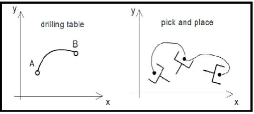
Fig. 2. Manipulator

Fig. 3. Object Tracing

Specifying Positions

A position in space may be denoted by a triple of numbers:

Position itself is a physical quantity independent of any frame. However it is often useful to express the position of a point in space relative to some frame. The left superscript on AP denotes the frame {A} in which the position is expressed. If one considers a different base frame {B}, the location of the physical point P does not change, however the triple of reals (i.e. BP) that denote its position in the new coordinates system of {B} certainly do

A

P≠B P

In fact, as we shall see later,

A

P = A PBorg +B P

Where A PBorg denotes the position of the origin of {B}

expressed in frame {A}.

Specifying Orientations

A single point in space has no orientation. We are usually interested in describing the orientation in space of some rigid body (e.g. robot end effector). The approach is to attach a frame fixed to the body. Associate the coordinate system (XA;

YA; ZA) to the inertial frame of reference {A}. The objects

(XA; YA; ZA) are unit vectors representing the coordinate

directions in {A}. By construction

Attach a frame to the body in space whose orientation we wish to describe. Denote this frame by {B}. Assume the situation that the origin of {B} is coincident to {A}, i.e. only orientation is important. Then associate the coordinate system (XB; YB;

ZB) to {B} so that the change in orientation from the inertial

frame to the new frame is a rotation of the basis (XA; YA; ZA)

to the new basis (XB; YB; ZB). Note that by convention, all

frames of reference are right-hand frames. The coordinate directions (XB; YB; ZB) fully determine the orientation of {B},

and we can describe this orientation with respect to the frame of reference {A} by the triple of vectors (AXB; AYB; AZB).

Compact notation is achieved by grouping the triple of vectors representing the orientation {B} relative to the frame of reference {A} by a matrix,

Such a matrix is known as a rotation matrix. How can one explicitly calculate the values of the entries of a rotation matrix? Let <X; Y> denote the usual inner (i.e. dot) product between two vectors.

Since YA and XB are unit vectors, their dot product is given by the cosine of the angle between them,

<YA; XB> = r21 = cos (Ѳ)

It is for this reason that the entries of a rotation matrix are known as direction cosines.

Properties of Rotation Matrices

All rotation matrices are orthogonal matrices RTR = I3. (i.e. both the rows and columns form an orthonormal basis; each row/column has length 1, an each are mutually perpendicular). Due to the symmetry of the inner product.

Recalling the orthogonal property one has,

Thus, the rotation matrix representing {B} with respect to {A} is the inverse of the matrix representing {A} with respect to {B}.

In fact rotation matrices form a group in matrix space termed the special orthogonal group,

The Group operations are, R.Q = RQ; Group multiplication R-1 = RT; Inverse operation

Rotation Matrices as Transform Mapping

We have seen that one use of a rotation matrix is to define the orientation of one frame with respect to another. Another use for a transformation matrix is as a transform mapping, i.e. a mapping that takes a vector quantity expressed in one frame, and expresses it in another. A representation of a vector V relies on a frame of reference

A vector may be represented in different frames of reference. For example if BV is known then,

Thus, the second interpretation is that the rotation matrix is a mapping between representations of free vectors.

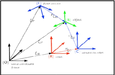
Frame analogy & transformations

Stochastic Map

Our knowledge of the spatial relationships among objects is inherently uncertain. A manmade object does not match its geometric model exactly because of manufacturing tolerances.

Even if it did, a sensor could not measure the geometric features, and thus locate the object exactly,

measurement errors. And even if it could,

sensor cannot manipulate the object exactly

because of hand positioning errors. These errors can be

29363 Pavleen S Bali et al. Obstacle avoidance &motion planning by stochastic pr

generation in the domain of embedded systems, mechatronics, artificial intelligence, robotics and machine learning

In fact rotation matrices form a group in matrix space termed

one use of a rotation matrix is to define the orientation of one frame with respect to another. Another use for a transformation matrix is as a transform mapping, i.e. a mapping that takes a vector quantity expressed in one frame, her. A representation of a vector V

A vector may be represented in different frames of reference.

Thus, the second interpretation is that the rotation matrix is a representations of free vectors.

Our knowledge of the spatial relationships among objects is inherently uncertain. A manmade object does not match its because of manufacturing tolerances. a sensor could not measure the geometric

exactly, because of

even if it could, a robot using the

exactly as intended, because of hand positioning errors. These errors can be

reduced to negligible limits for some tasks, by "pre engineering" the solution

environment and using specially equipment - but at great cost

rather than treat spatial uncertainty as a side issue in geometrical reasoning, we believe it must be treated as an intrinsic part of spatial representations. In this paper, uncertain spatial relationships will be tied togeth

called the stochastic map.

Fig. 4. Stochastic Frames

It contains estimates of the spatial relationships, their uncertainties, and their inter

structure will be described, followed by methods for extr information from it. Finally, a procedure will be given for building the map incrementally, as

obtained. To illustrate the theory, we will present an example of a mobile robot acquiring knowledge about its location and the organization of its environment by making sensor observations at different times and in different pl

Representation

In order to formalize the above ideas, we will define the following terms. A spatial relationship

the vector of its spatial variables,

and orientation of a mobile robot can be described by its coordinates, z and y, in a two dimensional cartesian reference frame and by its orientation, given as a rotation about the axis:

An uncertain spatial relationship,

by a probability distribution over its spatial variables

a probability density function that assigns a probability to each particular combination of the spatial variables, x:

P(x) = f(x) dx

Such detailed knowledge of the probability distribution is usually unnecessary for making decisions, such as whether the

Pavleen S Bali et al. Obstacle avoidance &motion planning by stochastic processes, spatial description, sensor integration and trajectory generation in the domain of embedded systems, mechatronics, artificial intelligence, robotics and machine learning

reduced to negligible limits for some tasks, by "pre-engineering" the solution - structuring the working environment and using specially-suited high-precision of time and expense. However, rather than treat spatial uncertainty as a side issue in geometrical reasoning, we believe it must be treated as an intrinsic part of spatial representations. In this paper, uncertain spatial relationships will be tied together in a representation

Stochastic Frames

It contains estimates of the spatial relationships, their uncertainties, and their inter-dependencies. First, the map structure will be described, followed by methods for extracting information from it. Finally, a procedure will be given for incrementally, as new spatial information is obtained. To illustrate the theory, we will present an example of a mobile robot acquiring knowledge about its location and the organization of its environment by making sensor observations at different times and in different places.

In order to formalize the above ideas, we will define the

spatial relationship will be represented by

spatial variables, x. For example, the position

and orientation of a mobile robot can be described by its and y, in a two dimensional cartesian reference given as a rotation about the z

spatial relationship, moreover, can be represented over its spatial variables - i.e., by a probability density function that assigns a probability to each particular combination of the spatial variables, x:

Such detailed knowledge of the probability distribution is usually unnecessary for making decisions, such as whether the

robot will be able to complete a given task (e.g. passing through a doorway). Furthermore, most measuring devices provide only a nominal value of the measured relationship, and we can estimate the average error from the sensor specifications. For these reasons, we choose to model an uncertain spatial relationship by estimating the first two moments of its probability distribution-the mean, x and the

covariance, C(x), defined as:

where E is the expectation operator, and 2 is the deviation from the mean. For our mobile robot example, these are:

Interpretation

For some decisions based on uncertain spatial relationships, we must assume a particular distribution that fits the estimated moments. For example, a robot might need to be able to calculate the probability that a certain object will be in its field of view, or the probability that it will succeed in passing through a doorway. Given only the mean, x, and covariance matrix, C(x), of a multivariate probability distribution, the principle of maximum entropy indicates that the distribution which assumes the least information is the normal distribution. Furthermore if the spatial relationship is calculated by combining many different pieces of information the central limit theorem indicates that the resulting distribution will tend to a normal distribution:

We will graph uncertain spatial relationships by plotting contours of constant probability from a normal distribution with the given mean and covariance information. These contours are concentric ellipsoids (ellipses for two dimensions) whose parameters can be calculated from the covariance matrix, C(x). It is important to emphasize that we do not assume that the uncertain spatial relationships are described by normal distributions. We estimate the mean and variance of their distributions, and use the normal distribution only when we need to calculate specific probability contours. In the figures in this paper, the plotted points show the actual locations of objects, which are known only by the simulator and displayed for our benefit. The robot's information is shown by the ellipses which are drawn centered on the estimated

mean of the relationship and such that they enclose a 99.9% confidence region (about four standard deviations) for the relationships.

Object Sensing

Throughout this paper we will refer to a two dimensional example involving the navigation of a mobile robot with three degrees of freedom. In this example the robot performs the following sequence of actions:

 The robot senses object #1

 The robot moves.

 The robot senses an object (object #2) which it determines cannot be object #l.

 Trying again, the robot succeeds in sensing object #1, thus helping to localize itself, object #1, and object #2.

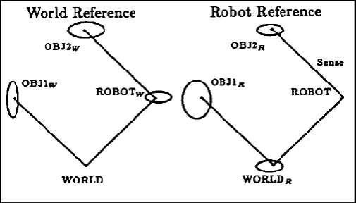
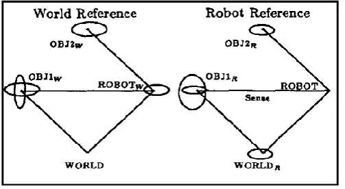
Fig. 5. The robot senses object 1 and moves

Figure shows two examples of uncertain spatial relationships - the sensed location of object #1, and the end-point of a planned motion for the robot. The robot is initially sitting at a landmark which will be used as the world reference location. There is enough information in our stochastic map at this point for the robot to be able to decide how likely a collision with the object is, if the motion is made. In this case the probability is vanishingly small. The same figure shows how this spatial knowledge can be presented from the robot's new reference frame after its motion. As expected, the uncertainty in the location of object #1becomes larger when it is compounded with the uncertainty in the robot's motion.

Fig. 6. The robot senses object 2

From this new location, the robot senses object #2. The robot is able to determine with the information in its stochastic map that this must be a new object and is not object #1which it observed earlier.

Fig. 7. The robot senses object 1 again

In Fig 7, the robot senses object #1again. This new sensor measurement acts as a constraint and is incorporated into the map, reducing the uncertainty in the locations of the robot, object #1 and Object #2.

Frame Analogy

We have used the term frame to this point as some coordinate system either translated or rotated relative to some base inertial coordinate system. In general we would like our frames both translated and rotated relative to the inertial system. So a general frame of reference {B} is fully specified by:

1.The position of the origin of the frame (expressed in the inertial frame of reference).

A

PBorg origin of frame {B} relative to frame {A}

2.The orientation of the frame, expressed as a rotation matrix relative to a reference frame.

A

BR Orientation of {B} relative to {A}

RB, R Orientation of {B} relative to inertial frame

Mapping between Frames

As in the pure rotation case, we are interested in deriving something like a rotation matrix that allows:

1. A description of an arbitrary frame in a concise format 2. The machinery to be able to transfer the description of vector quantities from one frame to another.

Assume an inertial frame {A}, and another frame {B} which is located somewhere in space and has arbitrary orientation to {A} (maybe {B} could be attached to the robot end effector for example). It is clear to see that any point P expressed in terms of frame {B}, i.e. BP, can be expressed in terms of frame {A} according to:

A

P: = ABRBP + APBorg

However, while this description solves 1, it provides a clumsy solution to 2. The trick here is to embed R3 into R4 by creating the matrix operator, denoted as AB T, by forming the matrix

where this matrix is termed a homogeneous transformation matrix, so that the previous expression for AP can be arrived at as:

The theory of homogeneous transformations is also heavily used in the Computer Graphics and Computer Vision fields, where the last row in ABT can be other than [0, 0, 0, 1] to effect

perspective and scaling operations. This more general machinery takes care of the special translation and pure-rotation cases.

Transformation Operator

A third interpretation of a homogeneous transform is as a transformation operator on a vector quantity in a single frame. Imagine we have a vector P expressed in a frame {A}, and we wish to rotate and translate that vector by some amount with respect to {A}. A homogeneous transform can be shown to achieve this operation. Although this operation seems quite different to the mapping interpretation introduced previously, the mathematics behind it is the same. Intuitively, one can see why this is the case:

1.Keeping the vector unmoved and expressing it in a frame that has been translated and rotated backwards" (i.e. the mapping between frames interpretation), is the same mathematically as

2.Keeping the frame unmoved and translating and rotating the vector forwards" (the operator interpretation). Since the operator interpretation is relevant to a single frame, we can drop the previous pre-super/subscripts, and simply use the notation T.

Robot kinematics

Introduction

Kinematics is the science of motion which treats motion without regard to the forces which cause it. Within the science of kinematics one studies the position, velocity, acceleration, and all higher order derivatives of the position variables. Hence, the study of the kinematics of robots refers to all geometrical and time-based properties of the motion. A very basic problem to be solved is: How to relate the robot’s

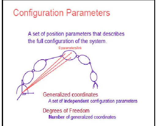
configuration or pose to the position and orientation of its end effector. A configuration of an n-degree of freedom robot is an n-vector (q,q...qn) 1 2, where each i q is either a rotational joint angle or a prismatic joint translation. This is known as the forward kinematics of the robot.

Fig. 8. Robot Kinematics

This is the static geometrical problem of computing the position and orientation of the end-effector of the robot. Specifically, given a set of joint angles, the forward kinematic problem is to compute the position and orientation of the TCP relative to the base frame. Sometimes we think of this as changing the representation of robot position from joint space description into a cartesian space description. The following problem is considered the inverse kinematics: Given the position and orientation of the end-effector of the robot, calculate all possible sets of joint angles which could be used to attain the given position and orientation. The inverse kinematics is not as simple as the forward kinematics. Because the kinematic equations are nonlinear, their solution is not always easy or even possible in a closed form. The existence of a kinematic solution defines the workspace of a given robot. The lack of a solution means that the robot cannot attain the desired position and orientation because it lies outside the robot’s workspace. In addition to dealing with static positioning problems, we may wish to analyse robots in motion. Often in performing velocity analysis of a mechanism it is convenient to define a matrix quantity called the jacobian of the robot. The jacobian specifies a mapping from velocities in joint space to velocities in cartesian space. The nature of this mapping changes as the configuration of the robot varies. At certain points, called singularities, this mapping is not invertible. An understanding of this phenomenon is important to designers and users of robots.

Definitions

• A robot maybe thought of as a set of bodies connect edinachain by joints.

• These bodies are called links.

• Joints form a connection between a neighbouring pairoflinks

Properties

• Normally robots consist of joints with one degree of freedom (1DOF).

• Revolute/prismatic joints

• n-DOF joints can be modelledasnjointswith1 DOF connected withn-1links of zero length

• Position in garobot in 3-space a minimum of six joints is required

• Typical robot consist of6joints • Join taxis are defined by lines in space

• Alinkcanbespecifiedbytwonumberswhichdefinetherelativel ocationofthetwo joint axes in space: link leng than d link twist

• Linklength:measuredalongthelinewhichismutuallyperpendic ulartobothaxes

• Link twist:measured in the plane defined by the perpendicular axis

Link Connection Description by Denavit-Hartenberg Notation

Neighbouring links have a common joint axis between them Parameters:

• Distance along common axis from one link to the other (link offset)

• Amount of rotation about this common axis between one link and its neighbour (joint angle)

Fig. 9. The length and twist of a link

A serial link robot consists of as equence of links connected

together by actuated joints. For ann DOF robot, there will been joints and n links. Thebaseoftherobotislink0andis not

considered one of the (n=6) links. Link 1is connected to the base link by joint1. There is no joint at the end of the final link (TCP). The only significance of links is that they maintain affixed relationship between the robot joints at each end of the link. Any link can be characterized by two dimensions: the common normal distance ai (called link length) and the angle Ѳi(called link twist) between the axes in a plane perpendicular to ai (see Fig 9). Generally, two links are connected a teach join taxis.

The axis will have two normals to it, one for each link. The relative position of two such connected links is given by di, the distance between the normals along the joint axis, and Ѳi the angle between the normals measured in aplane normal to the axis. di and Ѳi are called the distance and the angle between the links, respectively. Inordertode scribe the relationship between links, we will assign coordinate systems (frames) to each link. We will first consider revolute joints in which Ѳi is

the joint variable. The origin of the frame of linki is set to beat the inter section of the common normal between the axes of jointsiandi+1andtheaxisofjointi+1.Incase of intersecting joint axes, the origin is at the point of intersection of the joint axes. If the axes are parallel, the origin is chosen to make the joint distance zero for the next link whose coordinate rig in is defined. The axis for linki will be aligned with the axis of jointi+ 1. The axis will be aligned with any common normal which exists and is directed along the normal from jointi to jointi + 1. In case of intersecting joints, the direction of the axis is parallel or antiparallel to the vector cross product zi-1xzi. Notice that this condition is also satisfied for the axis directed along the normal between joints i and i+ 1. Ѳi is zero for the i-th revolute joint when xi-1 and xi are parallel and have i-the same direction. In case of prismatic joint, the distance di is the joint variable. The direction of the joint axis is the direction in which the joint moves. The direction of the axis is defined but, un like a revolute joint, the position in space is not defined. In the case of a prismatic joint, the length ai has no meaning and is setto zero. The origin of the frame for a prismatic joint is coincident with the next defined link origin. The zaxis of the prismatic joint is aligned with theaxisofjointi+1.The xi axis is parallelor ant parallel to the vector cross product of the direction of the prismatic joint and zi. For a prismatic joint we will define the zero position when di=0. With the robot in its zero position, the positive sense of rotation or revolute jointsor displacement for prismatic joints can be decided and the sense of the direction of thez axis determined. The origin of the base link (zero) will be coincident with the origin of link 1 If it is desired to define a different reference frame, then the relationship between the reference and base frames can be described by affixed homogeneous transformation. At the end of the robot, the final displacement 6 or rotation Ѳ6 occurs

with respecttoz _5.The origin of the frame for

link6ischosentobecoincidentwiththat of the link 5 frame. If a tool (or end effector) is used who seorigin and axes do not coincide with the frame of link 6, the tool can be related by affixed homogeneous trans formation to link 6. Having assigned frames to all links according to the preceding scheme, we can establish the relationshipbetweensuccessiveframesi-1, I by the following rotations and translations:

(a)Ѳi=the angle between Xi-1 and Xi measured about Zi-1 (b)di=the distance from Xi-1 to Ximeasured along Zi-1 (c)ai=the distance from Zi-1 to Zi measured along Xi (d)αi= the angle between Zi-1 and Zi measured about Xi

Due to the authors of this method attaching frames to links, these four parameters are called the Denavit Hartenberg parameters (DH parameters).

Forward Kinematics

Forward kinematics refers to the use of

the kinematic equations of a robot to compute the position of

the end-effector from specified values for the joint parameters. Given the joint values of the robot within degrees of freedom, the homogenous matrix defining the position and orientation of the TCP is:

The vectors p,n,o,a are described in the base (world) frame. This mapping from robot coordinates to world coordinates is unique.

Forward kinematics: mapping from robot coordinates to world coordinates

Inverse Kinematics

The reverse process that computes the joint parameters that achieve a specified position of the end-effector is known as inverse kinematics. Given the position and orientation of the TCP with respect to the base frame calculate the joint coordinates of the robot which correspond it.

Inverse kine matics: mapping from world coordinates to robot coordinates

Trajectory generation & motion planning

Introduction

Scope: methods of computing a trajectory in multidimensional

space

Definition: trajectory refers to a time history of position,

velocity and acceleration for each degree of freedom.

Issues:

 Specification of trajectories

 Motion description easy for robot operators

 Start and end point

 Geometrical properties

 Representation of trajectories in the robot control

 Computing trajectories on-line (a trun time)

General considerations

 Motion of robot is described as motion of TCP (tool frame)

 Supports robot operator’s imagination

 Decoupling the motion description from any robot, end-effector (modularity)

 Exchange ability with other robots

 Supports the idea of moving frames (conveyer belt)

Basic problem: move the robot from the start position, given by the tool frame T_initial to the end position given by the tool frame T_final.

Spatial motionconstraints:

 Specification of motion might include so called via points

 Viapoints:intermediate points bet

 Weenstart and end points

Temporal motion constraints:

 Specification of motion might include elapsed time between via points

Requirements:

 Execution of smooth motions

 Smooth (motion) function:functionand its first derivativeis continuous

 Jerky motions increase wear on the mechanism (gears)and cause vibrations by exciting resonances of the robot.

There are two methods of path generation:

 Joints pace schemes: paths hapes in space and time are described in terms of functions of joint angles. This motion type is named Point-to-Pointmotion (PTP)

 Cartesian space schemes: path shapes in space and time are described in terms of functions of Cartesian co ordinates. This motion type is named Continuous Pathmotion (CP)

Trajectory Generation in Joint Space (PTP Motions)

 Path shape (in space and time) described in terms of functions of joint angles

 Description of path points (via points plus start and end point) interms of tool frames

 Each path point is converted in to joint angles by application of inverse kinematics

 Identifying as mooth function for each of then joints passing through the via points and ends at the target point

 Synchronisation of motion (each joint starts and ends at the same time)

 Joint which travels the longest distance defines the travel time (assuming same maximal acceleration for each joint)

 In between via points the shape of the path is complex if described in artesian space

 Joint space trajectory generation schemes are easy to compute

 Each joint motion is calculated independently from other joints

Many, actually infinite, smooth functions exist for such motions.

Four constraints on the (single) joint function q (t) are evident:

 Start configuration q(0) = qA, end configuration end B

q(tend) = qB

 Velocities q(0) = 0, q(tend)=0



Fig. 10. PTP motion between two points

Four constraints can be satisfied by a polynomial of degree 3 or higher.

In case of via points the velocity is not zero.

 Start configuration q(0) = qA, end configuration end q(tend)

= B

 Velocities q(0)=q0, q(tend) = qB

Choosing velocities by

 Robot user

 Automatically chosen by the robot control

Using these type of polynomials does not in general generate time optimal motions.

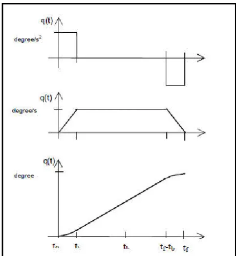
Linear function with parabolic blends:

Fig. 11. Path with trapezoidal velocity profile

Smooth motion constructed by adding parabolic blends to the linear function

Assumptions:

 Constant acceleration during blend

 Same duration for the (two) parabolic blends

 Therefore symmetry about the halfway point in time t

Trajectory Generation in Cartesian Space

Robot user would like to control the motion between start and end point several possibilities:

 Straight line motion (TCP follows a straight line)

 Circular motion (TCP follows a circle segment)

 Spline motion

 Inverse kinematics needs to be calculated at run time

 Computational expensive (depending on the robot)

Issues:

 Interpolation of TCP position (linear change of coordinates)

 Interpolation of orientation (linear change of matrix elements would fail)

Motion Planning

Motion planning (also known as the "navigation problem" or

the "piano mover's problem") is a term used in

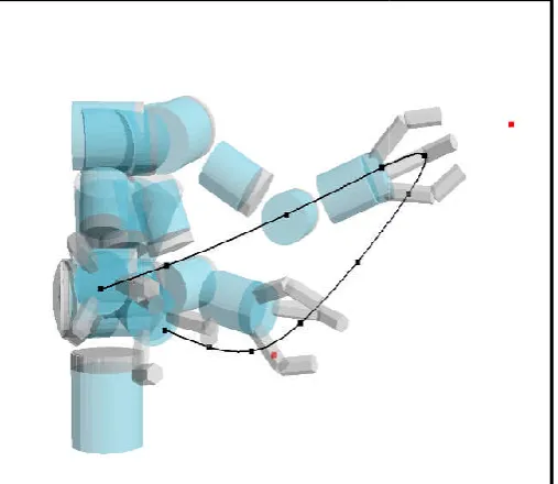
process of breaking down a desired movement task into discrete motions that satisfy movement constraints and possibly optimize some aspect of the movement. For example, consider navigating a mobile robot inside a building to a distant waypoint. It should execute this task while avoiding walls and not falling down stairs.

Fig. 12. Motion Planning

29369 Pavleen S Bali et al. Obstacle avoidance &

generation in the domain of embedded systems, mechatronics, artificial intelligence, robotics and machine learning

Smooth motion constructed by adding parabolic blends to the

Same duration for the (two) parabolic blends

point in time th

Robot user would like to control the motion between start and

line motion (TCP follows a straight line) motion (TCP follows a circle segment)

kinematics needs to be calculated at run time expensive (depending on the robot)

of TCP position (linear change of

of orientation (linear change of matrix

(also known as the "navigation problem" or the "piano mover's problem") is a term used in robotics for the process of breaking down a desired movement task into discrete motions that satisfy movement constraints and possibly optimize some aspect of the movement. For example, inside a building to a distant waypoint. It should execute this task while avoiding

A motion planning algorithm would take a description of these tasks as input, and produce the speed and turning commands sent to the robot's wheels. Motion planning algorithms might address robots with a larger number of joints (e.g., industrial manipulators), more complex tasks (e.g. manipulation of objects), different constraints (e.g., a car that can only drive forward), and uncertainty (e.g. imperfect models of the environment or robot). Motion planning has several robotics applications, such as autonomy,

in CAD software, as well as applications in other fields, such as animating digital characters,

intelligence, architectural design, study of biological molecules.

Configuration Space

A configuration describes the pose of the robot, and the configuration space C is the set of all possible configurations. For example:

 If the robot is a single point (zero

dimensional plane (the workspace), C is a plane, and a configuration can be represented using two parameters (x, y).

 If the robot is a 2D shape that can translate and rotate, the workspace is still 2-dimensional. However

Euclidean group SE (2) = the special orthogonal group configuration can be represented θ).

 If the robot is a solid 3D shape that can translate and rotate, the workspace is 3-dimensional, but C is the special Euclidean group SE (3)= R

requires 6 parameters: (x, y, z) for translation, angles (α, β, γ).

 If the robot is a fixed-base manipulator with N revolute joints (and no closed-loops), C is N

Free Space

The set of configurations that avoids collision with obstacles is called the free space Cfree. The complement of C

called the obstacle or forbidden region. Often, it is prohibitively difficult to explicitly compute the shape of C However, testing whether a given configu

efficient. First, forward kinematics

the robot's geometry, and collision detection geometry collides with the environment's geometry.

Robotic programing languages

Introduction:

Robot programming systems are the interface between the robot and the human user. The sop

interface is becoming very important as robots are applied to more and more demanding industrial applications. In considering the programming of manipulators, it is important to remember that they are typically only a minor part automated process. The term work cell is used to describe a local collection of equipment which may include one or more

Pavleen S Bali et al. Obstacle avoidance &motion planning by stochastic processes, spatial description, sensor integration and trajectory generation in the domain of embedded systems, mechatronics, artificial intelligence, robotics and machine learning

planning algorithm would take a description of these tasks as input, and produce the speed and turning commands sent to the robot's wheels. Motion planning algorithms might address robots with a larger number of joints (e.g., industrial complex tasks (e.g. manipulation of objects), different constraints (e.g., a car that can only drive (e.g. imperfect models of the Motion planning has several robotics autonomy, automation, and robot design software, as well as applications in other fields, such digital characters, video game artificial architectural design, robotic surgery, and the

A configuration describes the pose of the robot, and C is the set of all possible

int (zero-sized) translating in a 2-dimensional plane (the workspace), C is a plane, and a configuration can be represented using two parameters (x,

If the robot is a 2D shape that can translate and rotate, the dimensional. However, C is the special

R2 SO (2) (where SO (2) is special orthogonal group of 2D rotations), and a configuration can be represented using 3 parameters (x, y,

If the robot is a solid 3D shape that can translate and rotate, dimensional, but C is the special

R3 SO (3), and a configuration requires 6 parameters: (x, y, z) for translation, and Euler

base manipulator with N revolute loops), C is N-dimensional.

avoids collision with obstacles is . The complement of Cfree in C is

called the obstacle or forbidden region. Often, it is prohibitively difficult to explicitly compute the shape of Cfree.

However, testing whether a given configuration is in Cfree is

forward kinematics determine the position of collision detection tests if the robot's geometry collides with the environment's geometry.

obotic programing languages

Robot programming systems are the interface between the robot and the human user. The sophistication of such a user interface is becoming very important as robots are applied to more and more demanding industrial applications. In considering the programming of manipulators, it is important to remember that they are typically only a minor part of an automated process. The term work cell is used to describe a local collection of equipment which may include one or more

robots, conveyor systems, part feeders and fixtures. At the next higher level, work cells might be interconnected in factory wide networks so that a central control computer can control the overall factory flow.

Levels of Programing

Three levels of robot programming exist:

 Teach In programming

 Explicit robot languages

 Task level programming languages

Teach in Programming

The robot will be moved by the human user through interaction with a teach pendant (sometimes called teach box). Teach pendant are hand-held button boxes which allow control of each robot joint or of each cartesian degree of freedom. Today’s controllers allow alphanumeric input, testing and branching so that simple programs involving logic can be entered.

Explicit Robot Languages

With the arrival of inexpensive and powerful computers, the trend has been increasingly toward programming robots via programs written in computer programming languages. Usually these computer programming languages have special features which apply to the problems of programming robots. An international standard has been established with the programming language IRL (Industrial Robot Language, DIN 66312)

Task Level Programming

The third level of robot programming methodology is embodied in task-level programming languages. These are languages which allow the user to command desired sub goals of the task directly, rather than to specify the details of every action the robot is to take. In such a system, the user is able to include instructions in the application program at a significantly higher level than in an explicit programming language. A task-level programming system must have the ability to perform many planning tasks automatically. For example, if an instruction to grasp the bolt is issued, the system must plan a path of the manipulator which avoids collision with any surrounding obstacles, automatically choose a good grasp location on the bolt, and grasp it. In contrast, in an explicit robot language, all these choices must be made by the programmer. The border between explicit robot programming languages is quite distinct. Incremental advances are being made to explicit robot programming languages which help to ease programming, but these enhancements cannot be counted as components of a task-level programming system. True task-level programming of robots does not exist yet in industrial controllers but is an active topic of research.

Requirements of a Robot Programming Language

Important requirements of a robot programming language are:

 World modelling

 Motion specification

 Flow of execution

 Sensor integration

World Modelling

 Existence of geometric types to present

 joint angle sets

 Cartesian positions

 Orientations

 Representation of frames

 Ability to do math on structured types like frames, vectors and rotation matrices

 Ability to describe geometric entities like frames in several different convenient representations with the ability to convert between representations

Motion Execution:

 Description of desired motion (motion type, velocity, acceleration)

 Specifications of via points, goal points, corner smoothing parameters

 Ability to specify goals relative to various frames, including frames defined by the user and frames in motion (on a conveyor for example)

Flow of Execution:

 Support of concepts like testing and branching

 Looping, calls to subroutines

 Parallel processing, signal and wait primitives

 Interrupt handling

Sensor Integration:

 Interaction with sensors

 Integration with vision systems

 Sensor to track the conveyor belt motion

 Force torque sensor for force control strategies

DISCUSSION AND CONCLUSION

This paper presents a general theory for estimating uncertain relative spatial relationships between reference frames in a network of uncertain spatial relationships. Such networks arise, for example, in industrial robotics and navigation for mobile robots, because the system is given spatial information in the form of sensed relationships, prior constraints, relative motions, and so on. The theory presented in this paper allows the efficient estimation of these uncertain spatial relations. This theory can be used, for example, to compute in advance whether a proposed sequence of actions (each with known uncertainty) is likely to fail due to too much accumulated uncertainty; whether a proposed sensor observation will reduce the uncertainty to a tolerable level; whether a sensor result is so unlikely given its expected value and its prior probability of failure that it should be ignored, and so on. This paper applies state estimation theory to the problem of estimating parameters

of an entire spatial configuration of objects, with the ability to transform estimates into any frame of interest. The estimation procedure makes a number of assumptions that are normally met in practice. The angular errors are "small". This requirement arises because we linearize inherently nonlinear relationships. In Monte Carlo simulations, angular errors with a standard deviation as large as 5O gave estimates of the means and variances to within 1% of the correct values. Estimating only two moments of the probability density functions of the uncertain spatial relationships is adequate for decision making. We believe that this is the case since we will most often model a sensor observation by a mean and variance, and the relationships which result from combining many pieces of information become rapidly Gaussian, and thus are accurately modelled by only two moments. Although the examples presented in this paper have been solely concerned with spatial information, there is nothing in the theory that imposes this restriction. Provided that functions are given which describe the relationships among the components to be estimated, those components could be forces, velocities, time intervals, or other quantities in robotic and non-robotic applications.

REFRENCES

Alas, B., Cassell, A., Li, J., Meyyappan, M., and Callen, P. 2007. Friction of Partially Embedded Vertically Aligned Carbon Nano fibers Inside Elastomers. Applied Physics Letters, 91.

Ashley-Rollman, M. P., De Rosa, M., Srinivasa, S. S., Pillai, P., Goldstein, S.C., & Campbell, J. D. 2007a. Declarative Programming for Modular Robots. In Workshop on Self-Reconfigurable Robots/Systems and Applications at IROS '07.

Ashley-Rollman, M. P., Goldstein, S. C., Lee, P., Mowry, T. C. and Pillai, P. 2007b. Meld: A Declarative Approach to Programming Ensembles. In Proceedings of the IEEE International Conference on Intelligent Robots and Systems IROS'07.

Byrne, Seamus, 2008, December 22. Morphing Programmable Gadgets Could Soon Be a Reality. Retrieved February20, 2010from http://www.news.com.au/morphing-gadgets-could-soon-be-a-reality/story-0-1111118387380.

De Rosa, M., Goldstein, S. C., Lee, P., Campbell, J.D. and Pillai, P. 2008. Programming Modular Robots with Locally Distributed Predicates. In Proceedings of the IEEE International Conference on Robotics and Automation ICRA '08.

De Rosa, M., Goldstein, S.C., Lee, P., Pillai, P. and Campbell, J. 2009. ATale of Two Planners: Modular Robotic Planning with LDP. 2009 IEEE/RSJ International Conference on Intelligent Robots and Systems, IROS2009, October11, 2009 -October15.

*******