Using MCMC Probit Model to Value Coastal Beach Quality Improvement

doi:10.4236/jep.2011.21012 Published Online March 2011 (http://www.SciRP.org/journal/jep)

Using MCMC Probit Model to Value Coastal

Beach Quality Improvement

Zuozhi Li, Erda Wang, Jingqin Su, Yang Yu

School of Management, Dalian University of Technology, Dalian, China.

Email: LZZ200603@mail.dlut.edu.cn, edwang@dlut.edu.cn, jingqin@dlut.edu.cn, yuyang770727@hotmail.com

Received revised October 18th_{, 2010; revised November 25}th_{, 2010; accepted December 29}th_{, 2010.}

ABSTRACT

Dichotomous choice elicitation technique of contingent valuation method is broadly used in the research fields of envi-ronmental resource and recreational activity management. The binary choice type of questions are generally analyzed by using Logit or Probit probability distribution models in which a common analysis procedure is to apply MLE for estimating variable parameters before calculating the respondents’ willingness to pay. In this paper, a MCMC Gibbs sampling Probit model is adopted to maintain the three advantages it has in dealing with heteroscedasticity, high di-mension numerical integral and sample size restriction problems. The results revealed that the MCMC model and MLE Probit model are strikingly consistent, which suggests that the former is much simple and reliable estimation method. At the same time, the empirically based existence value estimation of coastal beach quality improvement in Dalian, China is RMBҰ168 per person.

Keywords: Value of Coastal Beach Quality, Markov Chain Monte Carlo (MCMC), Probit Model

1. Introduction

Contingent valuation technique is commonly used in environmental resource management fields, and monetized benefit measurement for improvements of environmental goods. Abundant research in beach nourishment has been conducted by applied economists [1-4]. In this paper, we are primarily concerned over the subject of coastal beach quality improvement with a particular emphasis on the relationship between tourism beach nourishment and tourists’ socioeconomic characteristics and the nature of their tourism activities as well. Beach conditions such as slope, width, mud, debris, congestion etc. are easily ob-servable and perceptively recognized by the tourists through photos presented to them. Tourists’ responses to the improved situation of coastal tourism resource quality is depended on a sequence of bidding value data to let respondent decide “Yes” or “No” regarding acceptance or rejection in an empirical survey. The type of binary dependent variable model in the empirical study can be estimated utilizing Logit or Probit probability distribu-tion which is firstly explored by Bishop and Heberlein (1979) with dichotomous choice (DC) elicitation model of CVM [5], which is called single-bounded DC.

The theoretical base of this method used in consumer welfare measurement is analyzed by Hanemann (1984) using Random Utility Maximization (RUM) [6]. With the support of the US Department of Commerce’s Na-tional Oceanic and Atmospheric Administration (NOAA) [7], RUM based utility difference DC model has been widely accepted and broadly extended. Traditionally, parameterized method of OLS or MLE is used, but it requires satisfying with homoscedastic assumption in order to be able to carry out a regression procedure in OLS, as well as a high dimension numerical integral which sometimes causes difficulty in solving consumer surplus based on MLE. Therefore, in this paper, we try to examine the performance of the non-parametric kernel heteroscedastic MCMC method by comparing its results against those generated by MLE in order to reveal the robustness of MCMC Gibbs sampling method.

2. Probit Regression Models

2.1. Heteroscedastic Regression Model

Bayesian treatment of the independent student t linear model, in which, variances of random error are embodied in heteroscedastic characteristics broken through the tra-ditional model to ensure a better statistical fitness (Ge-weke, 1993) [8]. The useful model is



2





, 0, 1,

i i i i i

y  x  N   i _,n



(1) Or

 





















2 1 1 1 1 1 1

, var , diag , , , , , , , , , , n n n

n k n

n n y y                             y X y

X x x

  

 

(2)

And the likelihood function is



  









2

2

1 2 2

1 1

, , ; , 2

exp 2

n n

n n

i i i

i i L y              _ _{  }  _ 





y X x   i   _ 



According to (1), there exist three hyper-parameters, and then the prior density is



, ,



1

 

2

  

3

         

Bayesian Markov chain Monte Carlo (MCMC) method is a comprehensive approach to solve high dimension numerical integral, because the analytical solution of exact posterior moments cannot be done, in the paper, the Gibbs sampler is used to draw a sequence of data. To use MCMC, the key point is to find the conditional posterior distributions. Hyper-parameter vector ω is not finally focused on, and it can be transformed into a single hy-per-parameter v to assigns an independent _2

 

_{v v} prior distribution to i terms. Furthermore, the jth

drawing data set is based on _ j 



_ j, j ,_ j,v j



_. In his study, the conditional posterior distributions are









1

1 2 -1 1 2 -1

1

2 1 2 -1

, N ,

                    _  _{ }        _  _    

X X G T G X y G T g

X X G T G

 

(3)



2



2





2



1

,

n

i i

i

u     



 

 





 n



(4)



2 2





_,



2



i i

u v v

    

   

  1



(5)

2.2. Probit Parameter Method

Probit model is one of binary choice probability distribu-tion models, which is usually used to solve dichotomous choice models of contingent valuation method (CVM) in valuing environmental resource or leisure activities. For binary choice model, given sampling from i = 1 to n, the explicit dependent variable is evaluated “0” or “1” as zi

in (6), which is representing the relationship between implicit dependent variable of continuous distribution as yiin (6) and explanation variables. Its basic format is as

(6).

0 if 0 1 if 0

i i i y z y     _

 (6)

In benefit measurement for improvements of tourism goods, tourists are asked information of willingness to pay (WTP) for environment or policy change. The WTP is a bidding value (explanation variable BID in this pa-per), furthermore, consumer surplus or environmental improvement value is measured through mean or median of WTP probability distribution after estimating parame-ters mentioned β above. Based on the utility difference model by Hanemann (1984), the implicit dependent va-riable yiexplained with a vector of independent variables

xi can be considered as the utility difference, and his

mentioned utility difference model is like (1) [6]. Ac-cording to his RUM assumption, given bidding value B, there is the probability expression as (7).



"Yes"









i i



 

i

P P B WTP P   y F y (7)

Traditional probability distribution of random error is paid attention to Logit or Probit model [5,6]. In Probit model, error accords with 0 and standard Normal distribution, whose cumulative density function (CDF) is as (8).

2 ₁

 



"Yes"





_i 1



 

_i

P P z  WTP   y (8) Integrated (7) with (8), WTP’s probability density function (PDF) and CDF could be written as Equation (9) and (10).

  

x





1 2



exp



 



2

f x     _  _

 X X  (9)





 







2



1, 1, ,

1 1 2 exp 2

i

P z i n x x

t d





   

 

_

X 





t (10)

Through MLE function (11), coefficient parameters β

can be estimated.

 





 





0

1n n i1n 1 i 1n 1

i

L z x z x







_ _  _   _ (11)

2.3. MCMC Probit Regression Model

In Probit model, i is distributed as standard normal

be- 

low, all of n original samples (yi, i = 1 to n) are revalued

for estimating the hyper-parameters.

The Gibbs sampling MCMC steps can be organized as follows.

1) The initial value is conveniently

assigned using OLS results with  ₀



₂



 0

, 



 

 0





1

,



   X X X y





 





 







0 2   _{ }  _  

   y X y X

 0

_

_

1 1,1, ,1_n

 _



n k , as well as

and v = 200 is a fixed value for sim-plifying calculation.

2) Given _ j 



_ j, j ,_ j,v j



_{to sample in step} j. Referred to z_i, i1, ,_ n in (6) to sample _y j

1

i

z

from normal distribution for left zero-truncation if  and right zero-truncation if z_i 0.



3) Draw _j1 conditional on _ j _{and } j _using

 j

 and (3), which means calculating the mean and variance of _j1 depended on _ j _{in last loop.}

4) Draw _j1 conditional on _j1 and _ j us-ing (4), which means decidus-ing in (4) after

com-puting , randomly drawing

and using

j1  1  j   j1 j1

 

_ 1

  j

y x





  



2 _n

 _ j _.

5) Draw _j1 conditional on _j1 and _j1 using (5), which means deciding in (5) after

computing , randomly

drawing and using . j1



j

 



 



v1

 

_{ }

 1

1 1 

 _  _{ } j

j _y j _x



_j1 1 2



6) Express a sampling route from step (2-5), repeat the route 3000 times, and obtain Markov chain {s1001, s1002, , s3000} after deleting the first 1000 set of data. 

In this process, a Bayesian regression approach is pre-sented for the chief purpose of getting hyper parameters β. According to the steps above, the Mean [β(1001)_{, β}(1002)_, , β(3000)_{], a point estimator of β, can be easily achieved.} Hereto the estimated βof MCMC approach together with β of MLE point estimator are obtained in use to value WTP of coastal beachquality improvement below.



3. WTP Estimators

Transform Equation (1) to (12) after retaining variable BID and calculating the remainder to get estimated con-stant α replaced explained variables with respective means.

ˆ ˆ

ˆ _x

y   x (12) Using the symmetrical property of the PDF curve for a standard normal distribution, we can set up F(y) = 0.5 in (7), from which the WTP median of equation (12) can be computed based on (13). Using Equations of (9) and (12), WTP mean can be obtained as through Equation (14).





_ˆ ˆ

x

Median WTP    (13)





  







2

ˆ _{1 2}

ˆ ˆ

ˆ ˆ

exp 2

x

x x

Median WTP X

x dx x

             _{ }  _{ }    



(14)

4. Statistical Analyses

4.1. Variables and Empirical Data

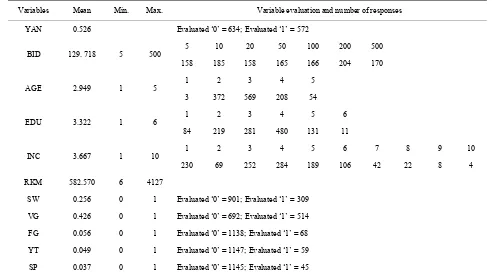
Tourism site survey was conducted from September 25 to October 10 in 2009 lasting for 15 days. Of which one week (Oct.1 - 7) is the Chinese national holiday that is so-called “golden week” period. The selected survey sites included four primary tourism sites in Dalian of northeastern China, including Tiger Beach Park, Fujiaz-huang Bathing Beach, Xinghai Square Beach, and Xing-hai Park. A pilot survey was conducted for pretest pur-pose before a formal interview survey was implemented. The survey sampled 1 276 individual tourists, of which 1 206 observations are valid responses after eliminating those incomplete survey response questionnaire. Thus, the effective survey response rate was 94.5%. The statis-tical descriptive information is listed in Table 1.

Variable YAN is binary choice dependent variable which is specified as ‘1’ given a “Yes” response, and ‘0’ for “No” response. BID is the priority variable which represents WTP of individual interviewee and it is la-beled as 7-levels of payment including Ұ5, Ұ10, Ұ20,

[image:4.595.50.543.102.377.2]

Table 1. The variables and descriptive statistics of survey data.

Variables Mean Min. Max. Variable evaluation and number of responses

YAN 0.526 Evaluated ‘0’ = 634; Evaluated ‘1’ = 572

5 10 20 50 100 200 500

BID 129. 718 5 500

158 185 158 165 166 204 170

1 2 3 4 5 AGE 2.949 1 5

3 372 569 208 54

1 2 3 4 5 6 EDU 3.322 1 6

84 219 281 480 131 11

1 2 3 4 5 6 7 8 9 10

INC 3.667 1 10

230 69 252 284 189 106 42 22 8 4

RKM 582.570 6 4127

SW 0.256 0 1 Evaluated ‘0’ = 901; Evaluated ‘1’ = 309

VG 0.426 0 1 Evaluated ‘0’ = 692; Evaluated ‘1’ = 514

FG 0.056 0 1 Evaluated ‘0’ = 1138; Evaluated ‘1’ = 68

YT 0.049 0 1 Evaluated ‘0’ = 1147; Evaluated ‘1’ = 59

SP 0.037 0 1 Evaluated ‘0’ = 1145; Evaluated ‘1’ = 45

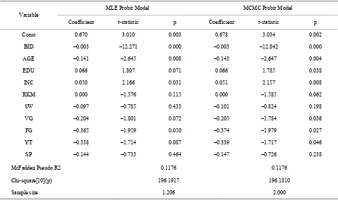
4.2. Results and Discussion

Based on Equations of (12), (13) and (14), the median WTP and mean WTP can be computed through using explanation variables show in Table 2, respectively,

where and

.



MLE





MLE



166.99

Mean WTP Median WTP



WTPMCMC



Median WTP



MCMC



168.20

 Mean

In Table 2, statistical tested were conducted to evalu-ate the regression model performance. It turns out that there are three asymptotically equivalent statistical tests including the likelihood ratio statistic, the Wald statistic, and the Lagrange multiplier statistic, which can measure goodness-of-fit and joint significance of all coefficients except the constant, but McFadden pseudo R2 _{and the} likelihood ratio test are commonly used. In these two models, the test results are almost identical with each other. McFadden pseudo R2 _{and the likelihood ratio can} be used to evaluate a model’s goodness-of-fits, and they all reach excellent level of significance in both models. T-test indicates that all explanatory variables reach 0.10 or better statistical significance except for variables of SW and SP. These highly consistent results suggest that the MCMC Probit model is effective method for DC- CVM type of analysis.

In estimating for both MLE parameters and hy-per-parameters of MCMC, two different models were used and both got consistent t-statistics as p-value indi-cated, which suggest that all those main estimators are

acceptable for the WTP estimations. Thus, in case a re-searcher is mainly interested in the study procedure to deal with complicated problems, a non-parameter esti-mation program should be recommended.

Connotation reflected through coefficients of explana-tory variables transmits the information that BID, AGE, and activities variables are negatively correlated with latent utility difference. The negative signs of coeffi-cients have different meaning for WTP measurement because BID’s is a denominator and the other explana-tory variables are embedded in the numerator of WTP calculation. Coefficient modulus of BID expresses an inverse ratio relationship with WTP, while the other ex-planatory variables are truly negative correlations with WTP.

5. Conclusions

[image:5.595.58.537.101.385.2]

Table 2. Probit model estimation and comparison.

MLE Probit Model MCMC Probit Model

Variable

Coefficient t-statistic p Coefficient t-statistic p

Const 0.670 3.010 0.003 0.678 3.034 0.002

BID –0.003 –12.271 0.000 –0.003 –12.842 0.000

AGE –0.141 –2.645 0.008 –0.143 –2.647 0.004

EDU 0.066 1.807 0.071 0.066 1.785 0.038

INC 0.050 2.166 0.031 0.051 2.157 0.008

RKM 0.000 –1.576 0.115 0.000 –1.585 0.062

SW –0.097 –0.785 0.433 –0.101 –0.824 0.198

VG –0.204 –1.801 0.072 –0.205 –1.784 0.036

FG –0.365 –1.959 0.050 –0.374 –1.979 0.027

YT –0.338 –1.714 0.087 –0.339 –1.717 0.046

SP –0.144 –0.733 0.464 –0.147 –0.726 0.238

McFadden Pseudo R2 0.1176 0.1176

Chi-square[10](p) 196.1917 196.1810

Sample size 1,206 2,000

As well as, a MCMC Gibbs sampling model holds better qualities because of the three advantages in dealing with heteroscedasticity, high dimension numerical inte-gral and sample size restriction problems. Parametric model based on OLS or MLE test procedures is widely applied for estimation of consumer surplus although the existence of heteroscedasticity does not fit in OLS and a high dimension numerical integral is also difficult to be solved using traditional parametric method. The non- parametric model using MCMC has been gradually rec-ognized as a handy method for estimating regression models. In the process, applying the MCMC Gibbs sam-pling to get hyper-parameters estimators is well received [9,10]. However, it is worth of noting the importance that it is necessary to get the conditional posterior distribu-tions.

The authors used the utility difference model to mate environmental resources via comparing and esti-mating a non-parametric regression model with 2000 enlarged samplers. Analyzed the regression coefficients, the finding is that education and income represent similar elasticity implication, which is the opposite of age and activities. The result indicates that the existence value of the coastal beach environmental quality improvement in Dalian, China is RMB Ұ168 per person, and this result is so consistent with the one obtained from using a tradi-tional method.

REFERENCES

[1] V. K. Smith, X. Zhang and R. B. Palmquist, “Marine Debris, Beach Quality, and Non-Market Values,”

Envi-ronmental and Resource Economics, Vol. 10, No. 3, 1997,

pp. 223-247. doi:10.1023/A:1026465413899

[2] J. C. Whitehead, C. F. Dumas, J. Herstine, J. Hill and B. Buerger, “Valuing Beach Access and Width with Re-vealed and Stated Preference Data,” Marine Resource

Economics, Vol. 23, No. 2, 2008, pp. 119-135.

[3] C. E. Landry, A. G. Keeler and W. Kriesel, “An Eco-nomic Evaluation of Beach Erosion Management Alter-natives,” Marine Resource Economics, Vol. 18, No. 2, 2003, pp. 105-127.

[4] C. Oh, A. W. Dixon, J. W. Mjelde and J. Draper, “Valu-ing Visitors’ Economic Benefits of Public Beach Access Points,” Ocean and Coastal Management, Vol. 51, No. 12, 2008, pp. 847-853.

doi:10.1016/j.ocecoaman.2008.09.003

[5] R. C. Bishop and T. A. Heberlein, “Measuring Values of Extra-market Goods: Are Indirect Measures Biased,”

American Journal of Agricultural Economics, Vol. 61,

No. 5, 1979, pp. 926-930.

doi:10.1016/j.ocecoaman.2008.09.003

[6] W. M. Hanemann, “Welfare Evaluations in Contingent Valuation Experiments with Discrete Responses,”

Amer-ican Journal of Agricultural Economics, Vol. 66, No. 3,

1984, pp. 332-341.

and H. Schuman, “Report of the NOAA Panel on Con-tingent Valuation,” 1993.

http://www.darrp.noaa.gov/library/pdf/cvblue.pdf [8] J. Geweke, “Bayesian Treatment of the Independent

Stu-dent t Linear Model,” Journal of Applied Econometrics, Vol. 8, No. 1, 1993, pp.19-40.

doi:10.1002/jae.3950080504

[9] S. Chib and E. Greenberg, “Markov Chain Monte Carlo

Simulation Methods in Econometrics,” Econometric

Theory, Vol. 12, No. 3, 1996, pp. 409-431.

doi:10.1017/S0266466600006794