Tests for conditional heteroscedasticity with functional data and goodness of fit tests for FGARCH models

Munich Personal RePEc Archive

Tests for conditional heteroscedasticity

with functional data and goodness-of-fit

tests for FGARCH models

Rice, Gregory and Wirjanto, Tony and Zhao, Yuqian

University of Waterloo, University of Waterloo, University of

Waterloo

31 March 2019

TESTS FOR CONDITIONAL HETEROSCEDASTICITY WITH FUNCTIONAL DATA AND GOODNESS-OF-FIT TESTS FOR FGARCH MODELS

GREGORY RICE∗, TONY WIRJANTO∗ AND YUQIAN ZHAO∗

∗_{Department of Statistics and Actuarial Science, University of Waterloo, Canada}

Abstract. Functional data objects that are derived from high-frequency financial data often

exhibit volatility clustering characteristic of conditionally heteroscedastic time series. Versions of functional generalized autoregressive conditionally heteroscedastic (FGARCH) models have recently been proposed to describe such data, but so far basic diagnostic tests for these models are not available. We propose two portmanteau type tests to measure conditional heteroscedasticity in the squares of financial asset return curves. A complete asymptotic theory is provided for each test, and we further show how they can be applied to model residuals in order to evaluate the adequacy, and aid in order selection of FGARCH models. Simulation results show that both tests have good size and power to detect conditional heteroscedasticity and model mis-specification in finite samples. In an application, the proposed tests reveal that intra-day asset return curves exhibit conditional heteroscedasticity. Additionally, we found that this conditional heteroscedasticity cannot be explained by the magnitude of inter-daily returns alone, but that it can be adequately modeled by an FGARCH(1,1) model.

JEL Classification:C12, C32, C58, G10

Keywords:Functional time series, Heteroscedasticity testing, Model diagnostic checking, High-frequency volatility models, Intra-day asset price

1. Introduction

Since the seminal work of Engle (1982) and Bollerslev (1986), generalized autoregressive

con-ditionally heteroscedastic (GARCH) models and their numerous generalizations have become

a cornerstone of financial time series modeling, and are frequently used as a model for the

volatility of financial asset returns. As the name suggests, the main feature that these models

account for is conditional heteroscedasticity, which for an uncorrelated financial time series can

be detected by checking for the presence of serial correlation in the series of squared returns of

the asset. This basic observation leads to several ways of testing for the presence of conditional

heteroscedasticity in a given time series or series of model residuals by applying portmanteau

tests to the squared series. Such tests have been developed by McLeod and Li (1983) and Li and

Mak (1994) to test for conditional heteroscedasticity and perform model selection for GARCH

models as well as autoregressive moving average models with GARCH errors. Diagnostic tests

of this type are summarized in the monograph by Li (2003), and with a special focus on GARCH

models in Francq and Zakoïan (2010). Many of these methods have also been extended to

mul-tivariate time series of a relatively small dimension; see also Francq and Zakoïan (2010), Tse

and Tsui (1999), Tse (2002), Duchesne and Lalancette (2003), Kroner and Ng (1998), Bauwens

et al. (2006), and Cataniet al. (2017).

In many applications, dense intra-day price data of financial assets are available in addition to

the daily asset returns. One way to view such data is as daily observations of high dimensional

vectors (consisting of hundreds or thousands of coordinates) that may be thought of as discrete

observations of an underlying noisy intra-day price curve or function. We illustrate with the data

that motivate our work and will be further studied below. On consecutive daysi_{∈ {}1, . . . , N_}, observations of the price of an asset, for instance the index of Standard & Poor’s 500, are available

at intra-day times u, measured at a 1-minute (or finer) resolution. These data may then be represented by a sequence of discretely observed functions_{Pi(u) : 1 ≤i≤T, u∈[0, S]}, with

Sdenoting the length of the trading day. Transformations of these functions towards stationarity that are of interest include the horizonhlog returns,Ri(u) = logPi(u)−logPi(u−h), where

his some given length of time, such as five minutes. For a fixed h, on any given trading day

to Bosq (2000), Ramsay and Silverman (2006), and Horváth and Kokoszka (2012) for a review

of functional data analysis and linear functional time series. Studying such data through the

lens of a functional data analysis has received considerable attention in recent years. The basic

idea of viewing transformations of densely observed asset price data as sequentially observed

stochastic processes appears in studies such as Barndorff-Nielson and Shepard (2004), Müller

et al. (2011) and Kokoszka and Reimherr (2013), among others.

Curves produced as described above exhibit a non-linear dependence structure and volatility

clustering reminiscent of GARCH-type time series. Recently functional GARCH (FGARCH)

models have been put forward as a model for curves derived from the dense intra-day price

data, beginning with Hörmannet al. (2013), who proposed an FARCH(1) model, which was

generalized to FGARCH(1,1) and FGARCH(p, q) models by Aueet al., (2017), and Cerovecki

et al. (2019), respectively. An important determination an investigator may wish to make

before she employs such a model is whether or not the observed functional time series exhibits

substantial evidence of conditional heteroscedasticity. To the best of our knowledge, there is

no formal statistical test available to measure conditional heteroscedasticity in intra-day return

curves or generally for sequentially observed functional data. Additionally, if an FGARCH

model is employed, it is desirable to know how well it fits the data, and whether or not the

orderspandq selected for the model should be adjusted. This can be addressed by testing for remaining conditional heteroscedasticity in the model residuals of fitted models.

In this paper, we develop functional portmanteau tests for the purpose of identifying conditional

heteroscedasticity in functional time series. Additionally, we consider applications of the

pro-posed tests to the model residuals from a fitted FGARCH model that can be used to evaluate

the model’s adequacy and aid in the order selection. The development of this later application

entails deriving joint asymptotic results between the autocovariance of the FGARCH

innova-tions and the model parameter estimators that are of independent interest. Simulation studies

presented in this paper confirm that the proposed tests have good size and are effective in

iden-tifying functional conditional heteroscedasticity as well as mis-specification of FGARCH-type

models. In an application to intra-day return curves derived from dense stock price data, our

tests suggest that the FGARCH models are adequate for modeling the observed conditional

heteroscedasticity across curves.

This work builds upon a number of recent contributions related to portmanteau and

goodness-of-fit tests for functional data. Gabrys and Kokoszka (2007) were the first to consider white noise

tests for functional time series, and their initial approach was based on portmanteau statistics

applied to finite-dimensional projections of functional observations. Horváth et al. (2013)

developed a general strong white noise test based on the squared norms of the autocovariance

operators for an increasing number of lags. General weak white noise tests that are robust

to potential conditional heteroscedasticity were developed in Zhang (2016) and Kokoszka et

al. (2017). Zhang (2016), Gabrys et al. (2010) and Chiou and Müller (2007) also consider

goodness-of-fit tests based on model residuals, with the first two being in the context of modeling

functional time series.

The remainder of the paper is organized as follows. In Section 2 we frame testing for

condi-tional heteroscedasticity as a hypothesis testing problem, and introduce test statistics for this

purpose. We further present the asymptotic properties of the proposed statistics, and show

how to apply them to the model residuals of the FGARCH models for the purpose of model

validation/selection. Some details regarding the practical implementation of the proposed tests

and a simulation study evaluating their performance in finite samples are given in Section 4.

An application to intra-day return curves is detailed in Section 5, and concluding remarks are

made in Section 6. Proofs of the asymptotic results are collected in appendices following these

main sections.

We use the following notation below. We letL2_[0,1]d _{denote the space of real valued square} integrable functions defined on unit hypercube[0,1]d_{with normk·kinduced by the inner product}

hx, yi = R1

0 · · ·

R1

0 x(t1, ..., td)y(t1, ..., td)dt1. . . dtd for x, y ∈ L2[0,1]d, the dimension of the

domain being clear based on the input function. Henceforth we write R

instead of R1

0. We

often consider kernel integral operators of the formg(x)(t) =R

g(t, s)x(s)dsforx∈L2_[0,1],

where the kernel functiong is an element ofL2_[0,1]2_{. We useg}(k)_{(x)(t)to denote thek-fold}

convolution of the operatorg. The filtration_Fi is used to denote the sigma algebra generated

by the random elements_{Xj, j ≤i}. We letC[0,1]denote the space of continuous real valued functions on[0,1], with norm defined forx _∈ C[0,1]as_kx_k∞ = supy∈[0,1]|x(y)|. We letχ2K denote a chi-square random variable withK degrees of freedom, and useχ2

quantile. _{k · k}E denotes the standard Euclidean norm of a vector inRd. We use{xi}to denote the sequence_{xi}i∈N, or{x_i}_i∈Z, with the specific usage of which being clear in context.

2. Tests for functional conditional heteroscedasticity

Consider a stretch of a functional time series of lengthN,X1(t), ..., XN(t), which is assumed to have been observed from a strictly stationary sequence _{Xi(t), i ∈ Z, t ∈ [0,1]} of stochastic processes with sample paths in L2_{[0,1]. For instance, below X}

i(t) denotes the intra-day log returns derived from densely observed stock prices on day i at intraday time t

where t is normalized to be in the unit interval. In this paper, we are generally concerned with developing tests that differentiate such series of curves, or model residuals, exhibiting

conditional heteroscedasticity from those that are strong functional white noises.

As emphasized by Engle (1982), conditional heteroscedasticity is generally characterized by

dependence of the conditional variance of an observed scalar time series on the magnitude of

its past values, which manifests itself in serial correlation in the squares of the series. This

leads one to consider the following definition of conditional heteroscedasticity for functional

observations:

Definition 2.1. [Functional Conditional Heteroscedasticity] We say that a sequence _{Xi} is conditionally heteroscedastic inL2_{[0,1]if it is strictly stationary,E[X}

i(t)|Fi−1] = 0, and

cov(X_i2(t), X_i2_+h(s))₆= 0,

for someh≥1, where the equality above is understood to be in theL2_[0,1]2_sense.

Recently, several models have been proposed in order to model series of curves exhibiting

conditional heteroscedasticity. Notably, the functional ARCH(1) and GARCH(1,1) processes

were put forward by Hörmann et al. (2013) and Aueet al. (2017), respectively, and take the

form

Xi(t) = σi(t)εi(t), Eε2i(t) = 1, t ∈[0,1], (2.1)

where

(2.2) FARCH(1) : σ_i2(t) = ω(t) +α(X_i2₋₁)(t) = ω(t) +

Z

α(t, s)X_i2₋₁(s)ds,

or FGARCH(1,1):

σ_i2(t) =ω(t) +α(X_i2₋₁)(t) +β(σ_i2₋₁)(t) = ω(t) +

Z

α(t, s)X_i2₋₁(s)ds+

Z

β(t, s)σ_i2₋₁(s)ds,

respectively. Here ω(t)is a non-negative intercept function, and α(t, s) andβ(t, s)are non-negative kernel functions. General FGARCH(p, q) models are discussed in Cerovecki et al. (2019), in which they also provide natural conditions under which these models admit strictly

stationary and non-anticipative solutions.

We frame testing for conditional heteroscedasticity as a hypothesis testing problem of

H0: The sequence{Xi(t)}is independent, and identically distributed, versus

HA: The sequence of{Xi(t)}is conditionally heteroscedastic given in Definition 2.1. Clearly it is not the case in general that rejecting_H0would directly lead us toHA, becauseXi(t) might instead be dependent or corrleated in the first moment. This concern can be alleviated

though if we test serial correlation in the sequence of squared curves as described in Definition

2.1.

In particular, we might then test _H0 versus HA by measuring the serial correlation in the

time series_kX1k2,...,kXNk2, or in the sequence of curves X12(t),...,XN2(t). Testing for serial correlation in the time series_kXik2can be viewed as measuring to what extent large in magnitude curves increase/decrease the likelihood of subsequent curves being large in magnitude, whereas

testing for serial correlation in the curvesX2

i(t)aims to more directly evaluate whether the data follow Definition 2.1. For some positive integerK, we then consider portmanteau statistics of the form

(2.3) VN,K =N

K

X

h=1

ˆ

ρ2_h, andMN,K =N K

X

h=1

kˆγhk2,

where ρˆh is the sample autocorrelation of the time series kX1k2,...,kXNk2, and γˆh(t, s) ∈

L2_[0,1]2 _{is the estimated autocovariance kernel of the functional time series X}2

i(t)at lag h, defined as

ˆ

γh(t, s) =

1

N

N−h

X

i=1

(X_i2(t)−X¯(2)(t))(X_i2_+h(s)−X¯(2)(s)),

withX¯(2)_{(t)) = (1/N)}PN

whereas the test statisticMN,K is the same as the portmanteau statistic defined in Kokoszkaet

al. (2017) applied to the squared functions.

Under_HA, we expect the statisticsVN,KandMN,Kto be large, and hence a consistent test can be obtained by rejecting_H0whenever they exceed a threshold calibrated according to their limiting

distributions under the null hypothesis. In order to establish the asymptotic distributions of each

portmanteau statistic under_H0, we impose the following moment condition.

Assumption 2.1. E_kXik8 <∞,i∈Z.

Under this assumption, the asymptotic distribution ofMN,Kdepends on the eigenvaluesλi, i≥

1of the kernel integral operator with kernel cov(X2

i(t), Xi2(s)), namely

λiϕi(t) =

Z

cov(X_i2(t), X_i2(s))ϕi(s)ds, (2.4)

where_{ϕi}is an orthonormal sequence of eigenfunctions inL2[0,1]. Assumption 2.1 guarantees that the eigenvalues_{λi}satisfy the condition thatP∞i=1λi <∞.

Theorem 2.1. If_H0 and Assumption 2.1 are satisfied, then we have

VN,K D

→χ2_K, asN → ∞,

(2.5)

and

MN,K D

→

K

X

h=1

∞

X

l,k=1

λlλkχ21(h, ℓ, k), asN → ∞,

(2.6)

where _{χ2

1(h, ℓ, k), 1 ≤ h ≤ K, 1 ≤ ℓ, k < ∞}are independent and identically distributed

χ2

1 random variables.

Theorem 2.1 shows that an approximate test ofH0 of sizeqis to reject ifVN,K > χ2K,1−q or if

MN,K exceeds the q’th quantile of the distribution on the right hand side of (2.6). The latter can be approximated in several ways, and in Section 4 below we describe a Welch-Satterthwaite

styleχ2_{approximation to achieve this.}

2.1. Consistency of the proposed tests. We now turn to studying consistency of each test

under_HA. In particular, we consider the asymptotic behavior ofVN,KandMN,K for sequences

{Xi}such that either: (a) they form a general weakly dependent sequences inL2[0,1]that are conditionally heteroscedastic as described by Definition 2.1, or (b) they follow a FARCH(1)

model as described in (2.2). We use the notion ofLp_{-m-approximability defined in Hörmann} and Kokoszka (2010) in order to describe general weakly dependent sequences, which covers

strictly stationary functional GARCH type processes under suitable moment conditions; see

Ceroveckiet al. (2019).

Theorem 2.2. If_{Xi}isL8-m-approximable andHAholds wherehin Definition 2.1 satisfies

1_≤h_≤K, then

MN,K p

→ ∞, N _{→ ∞}.

(2.7)

If in additionRR cov(X2

i(t), Xi2+h(s))dtds6= 0, then

VN,K p

→ ∞, N _{→ ∞}.

(2.8)

Remark 2.1. In typical financial applications we expect that the sequence of squared returns

are positively correlated, which may be interpreted in this setting as cov(X2

i(t),Xi2+h(s))≥0, for allt, s _∈[0,1],i.e. the covariance surface of the squared process at laghofX2

i(t)is strictly positive. Under this additional requirement the conditions for consistency ofMN,K andVN,K in Theorem 2.2 become equivalent.

Under the FARCH(1) model we can develop more precise results on the rate of divergence

of VN,K andMN,K. The following assumption ensures that a stationary and causal sequence satisfying (2.1) and (2.2) exists inL2_[0,1]:

Assumption 2.2. The sequence_{εi}in(2.1)is independent and identically distributed, and the

kernelα(t, s)in(2.2)is non-negative,_kα_k<1, and satisfies that there exists a constantτ >0

so that

E

Z Z

α2(t, s)ε2₀(s)dtds

τ /2

Theorem 2.3. Suppose that_{Xi}is the strictly stationary solution to the FARCH(1) equations

under Assumption 2.2 so that Assumption 2.1 holds, and letVi(t) =Xi2(t)−σ2i(t). ThenVi(t)

is a mean zero weak white noise inL2_{[0,1](see pg. 72 Bosq (2000)),}

VN,K

N

p

→

K

X

h=1

RR P∞

j=0Eα(j)(Vj)(t)α(j+h)(Vj)(s)dtds

2

RR P∞

j=0Eα(j)(Vj)(t)α(j)(Vj)(s)dtds

2 ,

(2.9)

and

MN,K

N

p

→

K

X

h=1

∞

X

j=0

Eα(j)(Vj)(t)α(j+h)(Vj)(s)

2

.

(2.10)

The right hand side of (2.10) is guaranteed to be strictly positive if RR α(t, s)Eω(t)(ε2 0(t)−

1)ω(s)(ε2

0(s)−1)dtds6= 0.

Remark 2.2. Theorem 2.3 shows that under an FARCH(1) model, the rate of divergence of

VN,K andMN,K depend essentially on the size of the functionα(t, s)as well as how this kernel projects onto the intercept term in the conditional variance ω(t) and the covariance of the squared errorε2

0(t). If for example

RR

α(t, s)E(ε2

0(t)−1)(ε02(t)−1)dtds= 0, then we do not

expect the tests to be consistent.

3. Diagnostic Checking for Functional GARCH Models

The conditional heteroscedasticity tests proposed above can also be used to test for the adequacy

of the estimated functional ARCH and GARCH models, and can aid in the order selection

of these models. We introduce this approach in the context of testing the adequacy of the

FGARCH(1,1) model, although one could more generally consider the same procedure applied

to the FGARCH(p, q) models using the estimation procedures in Cerovecki et al. (2019). To this end, suppose thatXi(t), 1 ≤ i ≤ N follows an FGARCH(1,1) model. To estimate ω(t), and the kernel functionsα(t, s)and β(t, s), following Aue et al. (2017) and Ceroveckiet al. (2019), we suppose that they have finite L-dimensional representations determined by a set of

basis functionsΦL ={φ1, φ2, . . . , φL}inL2[0,1]so that

ω(t) =

L

X

j=1

djφj(t), α(t, s) = L

X

j,j′₌₁

aj,j′φ_j(t)φ_j′(s), β(t, s) =

L

X

j,j′₌₁

bj,j′φ_j(t)φ_j′(s).

(3.1)

Under this assumption, estimating these functions amounts to estimating the coefficients in

their finite dimensional representations, which can be achieved by using, for example,

Quasi-Maximum Likelihood estimation (QMLE) or Least Squares estimation, as is typically employed

in multivariate GARCH models. To see this, under (3.1) we can re-express the FGARCH(1,1)

model in terms of the coefficients as

(3.2) s2

i =D+Ax2i−1+Bs2i−1

wherex2

i = [hXi2(t), φ1(t)i, . . . ,hXi2(t), φL(t)i]⊤, s2

i = [hσi2(t), φ1(t)i, . . . ,hσ2i(t), φL(t)i]⊤, the coefficient vector D = [d1, . . . , dL]⊤ ∈ RL, and the coefficient matrices A and B are

RL×L _{with(j, j}′_{)entries by aj,j}′ andb_j,j′, respectively. To estimate the vector of parameters

θ0 = (D⊤,vec(A)⊤,vec(B)⊤)⊤, Aue et al. (2017) propose a Least Squares type estimator

satisfying

ˆ

θN = arg min θ∈Θ

( _N X

i=2

(x2

i −s2i(θ))⊤(x2i −s2i(θ))

)

,

where Θ_{is a compact subset of} RL+2L2_{. Under certain regularity conditions, detailed at the}

beginning of Appendix B, it can be shown thatθˆN is a consistent estimator ofθ0, and in fact

√

N(ˆθN −θ0)satisfies the central limit theorem. This yields estimated functions given by

ˆ

ω(t) =

L

X

j=1

ˆ

djφj(t), αˆ(t, s) = L

X

j,j′₌₁

ˆ

aj,j′φ_j(t)φ_j′(s), βˆ(t, s) =

L

X

jj′₌₁

ˆ

bj,j′φ_j(t)φ_j′(s).

The functions φj can be chosen in a number of ways, including using a deterministic basis system such as polynomials, b-splines, or the Fourier basis, as well as using a functional

principal component basis; seee.g. Chapter 6 of Ramsay and Silverman (2006). Ceroveckiet

al. (2019) and Aueet al. (2017) suggest using the principal component basis determined by

the squared processesX2

i(t), which we also consider below. Given these function estimates, we can estimate recursivelyσˆ2

To test the adequacy of the FGARCH(1,1) model, we utilize the fact that if the model is well

specified then the sequence of model residuals εi(t), 1 ≤ i ≤ N, should be approximately independent and identically distributed, where

(3.3) εˆi(t) =

Xi(t)

ˆ

σi(t)

.

This suggests that we consider the portmanteau statistics constructed from the residuals

VN,K,ε =N

K

X

h=1

ˆ

ρε,h, andMN,K,ε =N K

X

h=1

kˆγε,hk2,

whereρˆε,his the sample autocorrelation of the scalar time serieskεˆ1k2, ...,kεˆNk2, and

ˆ

γε,h(t, s) =

1

N

N−h

X

i=1

ˆ

ε2_i(t)−1

ˆ

ε2_i+h(s)−1

.

(3.4)

A test of model adequacy of sizeqis to reject ifVN,K,ε > χ2K,1−qor ifMN,K,εexceeds the1−q’th quantile of the distribution on the right hand side of (2.6), where again this distribution must

be estimated from the squared residualsεˆ2

i(t). We abbreviate these tests below as being based on Vheuristic

N,K,ε andMN,K,εheuristic, since even under the assumption that that the model is correctly specified the residualsεˆi are evidently not independent and identically distributed due to their common dependence on the estimated parametersθˆN.

3.1. Accounting for the effect of parameter estimation. The approximate goodness-of-fit

tests proposed above provide a heuristic method to evaluate the model fit of a specified functional

GARCH type model, however we now aim at more precisely describing how the asymptotic

distribution ofMN,K,ε based on the model residualsεˆi(t)depends on the joint asymptotics of the innovation process and the estimated parametersθˆN. In this subsection, we focus only on quantifying this effect for the fully functional statistic MN,K,ε. Further, we assume that the parameter estimateθˆN is obtained by the Least Squares method proposed in Aue et al. (2017), although this could easily be adapted to the QMLE parameter estimate as well.

Given the regularity conditions stated Appendix B, it follows that

(3.5) √N(ˆθN −θ0)

d

→ NL+2L2(0, Q−1

0 H0⊤J0H0Q−01),

where_Np(0,Σ)denotes apdimensional normal random vector with mean zero and covariance matrixΣ. We use the notationσ2

i(t, θ)ands2i(θ)to indicate how each of these terms depends on the vector of parameters defined in (3.1). The termsJ0,H0, andQ0are respectively defined

as

J0 =E{[x20−s20][x20−s20]⊤}, H0 =E

∂˜s2 0(θ)

∂θ

, Q0 =E

(

∂˜s2 0(θ)

∂θ

⊤

∂˜s2 0(θ)

∂θ

)

.

LetGh : [0,1]2 →RL+2L 2

be defined by

Gh(t, s) =−E

1

σ2

i+h(s, θ0)

× ∂σ

2

i+h(s, θ0)

∂θ ×(ε

2

i(t, θ0)−1)

.

(3.6)

We further define the covariance kernels

Cε(t, s, u, v) =E{(ε2i(t)−1)(ε2i(s)−1)}E{(ε2i(u)−1)(ε2i(v)−1)},

and

C_h,gε,θ(t, s, u, v) = E

(ε2−h(t)−1)(ε20(s)−1)G⊤g(u, v)Q−01(

∂s2 0(θ0)

∂θ )

⊤_(x2 0−s20)

.

Theorem 3.1. Suppose that _{Xi} follows an FGARCH(1,1) model. Under the assumptions

detailed in Appendix B, there exists a sequence of non-negative coefficients _{ξ_i,K(ε,θ), i ≥ 1}

such that

MN,K,ε D

→

∞

X

i=1

ξ_i,K(ε,θ)χ2₁(i),

(3.7)

whereχ2

1(i), i≥ 1are independent and identically distributedχ2 random variables with one

degree of freedom. The coefficientsξ_i,K(ε,θ) are the eigenvalues of a covariance operatorΨ(_Kε,θ), defined in(B.1)below, that is constructed from kernels of the form

ψ(_K,h,gε,θ) (t, s,u, v) = Cε(t, s, u, v) +Ch,gε,θ(t, s, u, v) (3.8)

+C_g,hε,θ(u, v, t, s) +G_h⊤(t, s)Q−₀1H₀⊤J0H0Q−01Gg(u, v), 1≤h, g ≤K.

rigorous statement of this result is given in Appendix B along with the necessary assumptions

on the FGARCH model, which basically are taken to be strong enough to imply (3.5), and

that the solution _{Xi} of the FGARCH equations exists in C[0,1] with sufficient moments. These results may be easily generalized to FGARCH models of other orders, for instance, the

FARCH(1) model, which we study in the simulation section below.

4. Implementation of the tests and a simulation study

This section gives details on implementation of the proposed tests and evaluates the performance

of the proposed tests in finite samples. Several synthetic data examples are considered for this

purpose. A simulation study on diagnostic checking for the FGARCH model is also provided

in the last subsection.

4.1. Computation of test statistics and asymptotic critical values. In practice we only

ob-serve each functional data object Xi(t) at a discrete collection of time points. Often in fi-nancial applications these time points can be taken to be regularly spaced and represented as

TJ = {tj = j/J, j = 1, . . . , J} ⊂ (0,1]. Given the observations of the function Xi(tj),

tj ∈ Tj, we can estimate,e.g. the squared normkXik2 by a simple Riemann sum,

kXik2 =

1

J

J

X

j=1

X_i2(tj).

Other norms arising in the definitions ofVN,K and MN,K can be approximated similarly. For data observed at different frequencies, such as tick-by-tick, the norms and inner-products can

be estimated with Riemann sums or alternate integration methods as the data allows. In all of

the simulations below we generate functional observations onJ = 50equally spaced points in the interval[0,1].

The critical values of the null limiting distribution of VN,K can easily be obtained, but esti-mating the limiting null distribution of MN,K defined in (2.6) requires a further elaboration. One option is to directly estimate the eigenvalues of the kernel integral operator with kernel

cov(Xi2(t), Xi2(s))via estimates of the kernel. Here, for the sake of computational efficiency, we propose a Welch-Satterthwaite style approximation of the limiting distribution; see e.g.

Zhang (2013) and Kokoszkaet al. (2017). The basic idea of this method is to approximate the

limiting distribution in (2.6) by a random variableRK ∼βχ2ν, whereβandνare estimated so

that the distribution ofRK has the same first two moments as the limiting distribution on the right hand side of (2.6). IfMK denotes the random variable on the right hand side of (2.6),

µK = E(MK), andσ2K =var(MK), then in order that the first two moments ofRKmatch those ofMK we take

β = σ

2

K

2µK

and ν = 2µ

2

K

σ2

K

.

(4.1)

We verify below that

µK =K

Z

cov(X₀2(t), X₀2(t))dt

2

,

σ_K2 = 2K

Z Z

cov(X₀2(t), X₀2(s))dtds

2

.

(4.2)

These can be consistently estimated by

ˆ

µK =K

Z

1

N

N

X

i=1

(X_i2(t)−X¯(2)(t))2dt

!2

, and

ˆ

σ_K2 = 2K

Z

1

N

N

X

i=1

(X_i2(t)−X¯(2)(t))(X_i2(s)−X¯(2)(s))dtds

!2

,

whereX¯(2)_{(t) = (1/N)}PN

i=1Xi2(t). A test ofH0 with an approximate size ofq is to reject if

MN,K exceeds the1−qquantile of the distribution ofRK ∼βχˆ 2νˆ.

Similarly, in order to estimate the asymptotic critical values of MN,K,ε under the FGARCH model adequacy described in Theorem 3.1, we obtain the parametersβandνof approximated distribution by estimating,

µK =Trace(Ψ(Kε,θ)),

σ_K2 = 2Trace([Ψ(_Kε,θ)]2).

(4.3)

We can consistently estimate these terms using estimators of the form,

ˆ

µK = K

X

h=1

Z Z

ˆ

ψ_K,h,h(ε,θ) (t, s, t, s)dtds, and

ˆ

σ_K2 =

K

X

h,g=1

2

Z Z Z Z

whereψˆ_K,h,g(ε,θ) are consistent estimators of the kernelsψ_K,h,g(ε,θ) , which we define in the last subsection of Appendix B.

Calculating and storing such kernels, which can be thought of as 4-dimensional tensors, is

computationally intractable if J is large, which is commonly the case when considering

high-frequency financial data. For example, J=390 when using 1-minute resolution US stock market

data. To solve this problem, we use a Monte Carlo integration to calculate the integrals above

based on a randomly sparsified sample, with the sparse pointsJ∗_{determined by drawing from} a uniform distribution on[0,1]. Below we useJ∗ _{= 20points to estimate these integrals, which} seems to work well in practice.

4.2. Simulation study of tests for conditional heteroscedasticity. In this subsection we

present the results of a simulation study in which we evaluate the proposed tests for

func-tional condifunc-tional heteroscedasticity applied to simulated data sets. In particular, we consider

the following data generating processes (DGPs). Let _{Wi(t), t ∈ [0,∞), i ∈ Z} denote independent and identically distributed sequences of standard Brownian motions. We let

{ϕi(t), t∈[0,1], i∈ N}denote the standard Fourier basis. We then consider the following five DGPs:

(a) IID-BM:Xi(t) = Wi(t)

(b) FARCH(1): Xi(t)satisfies the FARCH(1) specification, with

α(x)(t) =

Z

12t(1₋t)s(1₋s)x(s)ds,

and ω = 0.01 (a constant function), and the innovation sequence εi(t) follows an Ornstein-Uhlenbeck process, which is also used in other FGARCH-type processes

throughout the paper:

(4.4) εi(t) = e−t/2Wi(et), , t∈[0,1].

(c) FGARCH(1,1): Xi(t)satisfies the FGARCH(1,1) specification, with

α(x)(t) =

Z

12t(1−t)s(1−s)x(s)ds, β(x)(t) =

Z

12t(1−t)s(1−s)x(s)ds,

ω = 0.01(a constant function), andεi(t)follows (4.4). (d) Pointwise (PW) GARCH(1,1): Xi(t)follows (2.1) with

σ2_i(t) =ω(t) +α(t)X_i2₋₁(t) +β(t)σ_i2₋₁(t)

whereα(t) = (t₋0.5)2_{+ 0.1andβ(t) = (t−0.5)}2_{+ 0.4.}

(e) FGARCH-BEKK model: Xi(t)satisfies

(4.5) Xi(t) =σi(εi)(t),

whereσ_i(·)(t)is a linear operator with a kernel functionσi(t, s), with

σi(t, s) =

2

X

ℓ,j=1

Hi(ℓ, j)ϕℓ(t)ϕj(s),

and

εi(t) =

2

X

ℓ=1

Zi,ℓϕℓ(t), Zi,ℓ iid

∼ N(0,1).

The matrixHifollows a BEKK multivariate GARCH specification

Hi2 =C⊤C+Aξi−1ξ⊤i−1A⊤+BHi2−1B⊤,

(4.6)

with

C =





1 0.3 0 1



, A= 



0.3 0.01 0.01 0.3



, andB = 



0.9 0.01 0.01 0.9



.

The process IID-BM satisfies_H0, while the remaining processes satisfyHA. The specific form

of the FARCH and FGARCH processes are inspired by Aueet al. (2017) and produce sample

paths that mimic high-frequency intraday returns. The FGARCH-BEKK process is meant to

model the situation in which the vector valued time series obtained by projecting the functional

series into a finite dimensional space satisfies a multivariate GARCH specification; see Engle

and Kroner (1995) and Francq and Zakoïan (2010). The existence of a stationary and causal

solution inL2_{[0,1]to (4.5) follows if the multivariate GARCH specification in (4.6) has such a}

Each sample of length N from the GARCH-type processes were produced after discarding a burn-in sample of length 50 starting from an initial innovation. In the simulation, we consider

samples sizes of125,250and500, which roughly match the number of trading days in a quarter,

half a year, one year, and two years, respectively.

Table 4.1 displays the percentage of rejections of_H0using the two proposed test statisticsVN,K andMN,K based on 1000 independent simulations from each DGPs for several choices of K and nominal levels of 10%, 5% and 1%. Both test statistics show reasonably good size in finite

samples that improve with increasingN, in accordance with Theorem 2.1. This also suggests that the Welch-Sattherwaite style approximation for the limiting distribution ofMN,Kperforms well.

Regarding the power of each test, we noticed that in general the test based onMN,K had greater power than the test based on VN,K for the examples considered in the simulation. Increasing

K in general reduces the power of the tests, which is expected in these examples, since the level of serial correlation in the squared processes is decreasing at higher lags. However, this

is not always the case when these test statistics are used as a diagnostic of fitted FGARCH

models below, since in that case serial correlation in the squared process is not necessarily

monotonically decreasing with increasing lags. Additionally, in the case of PWGARCH model,

the power ofVN,K test decays more slowly than theMN,K test asKincreases.

4.3. Simulation study of FGARCH goodness-of-fit tests. We now turn to a simulation study

of the proposed test statistics applied to diagnostic checking of FGARCH models as described

in Section 3. In particular, we generate data from the following three DGPs: the FARCH(1),

FARCH(2), and FGARCH(1,1). The specific FARCH(2) model considered is defined as

Xi(t) = σi(t)εi(t)

whereεi(t)is defined in (4.4) and,

σ_i2(t) =ω(t) +

Z

12(t_·(1₋t))(s_·(1₋s))X_i2₋₁(s)ds+

Z

12(t_·(1₋t))(s_·(1₋s))X_i2₋₂(s)ds.

For each simulated sample we then test for the model adequacy of the FARCH(1) model. When

the data follows the FARCH(1) specification, we expect the test to reject the adequacy of the

FARCH(1) model only a specified level of significance, while we expect that the adequacy of

Table 4.1. Empirical rejection rates of the tests for conditional heteroscedastic-ity usingVN,K andMN,K based on 1000 independent simulations at asymptotic levels of 10%, 5%, and 1%.

DGP: IID-BM FARCH(1) FGARCH(1,1) PWGARCH(1,1) FBEKK(1,1) Statistic: V_N,K M_N,K V_N,K M_N,K V_N,K M_N,K V_N,K M_N,K V_N,K M_N,K

K=1

N=125

10% 0.07 0.07 0.93 0.98 0.63 0.80 0.63 0.78 0.40 0.40 5% 0.04 0.04 0.91 0.97 0.56 0.75 0.56 0.73 0.32 0.33 1% 0.01 0.01 0.80 0.94 0.41 0.63 0.39 0.61 0.18 0.20

N=250

10% 0.07 0.07 1.00 1.00 0.89 0.97 0.90 0.96 0.70 0.71 5% 0.04 0.04 1.00 1.00 0.85 0.96 0.85 0.94 0.62 0.64 1% 0.01 0.01 0.99 1.00 0.75 0.92 0.76 0.91 0.49 0.51

N=500

10% 0.10 0.09 1.00 1.00 0.99 1.00 1.00 1.00 0.95 0.95 5% 0.05 0.05 1.00 1.00 0.99 1.00 0.99 1.00 0.92 0.92 1% 0.01 0.01 1.00 1.00 0.97 1.00 0.97 0.99 0.85 0.86

K=5

N=125

10% 0.07 0.08 0.81 0.92 0.67 0.89 0.68 0.90 0.59 0.60 5% 0.04 0.05 0.75 0.89 0.63 0.88 0.60 0.86 0.53 0.55 1% 0.01 0.02 0.60 0.83 0.52 0.81 0.50 0.79 0.41 0.44

N=250

10% 0.08 0.08 0.98 0.99 0.93 0.99 0.93 0.99 0.89 0.90 5% 0.04 0.05 0.98 0.99 0.91 0.99 0.89 0.99 0.87 0.88 1% 0.01 0.02 0.94 0.99 0.84 0.99 0.84 0.98 0.80 0.82

N=500

10% 0.09 0.09 1.00 1.00 1.00 1.00 0.99 1.00 0.99 1.00 5% 0.05 0.05 1.00 1.00 1.00 1.00 0.99 1.00 0.99 1.00 1% 0.01 0.02 1.00 1.00 0.99 1.00 0.99 1.00 0.98 0.99

K=10

N=125

10% 0.06 0.06 0.76 0.86 0.60 0.86 0.66 0.88 0.56 0.57 5% 0.03 0.03 0.68 0.82 0.55 0.82 0.59 0.85 0.49 0.50 1% 0.01 0.01 0.53 0.75 0.43 0.75 0.49 0.79 0.38 0.40

N=250

10% 0.08 0.08 0.97 0.99 0.90 0.99 0.90 0.99 0.91 0.92 5% 0.04 0.04 0.95 0.98 0.87 0.99 0.86 0.99 0.88 0.88 1% 0.01 0.01 0.92 0.97 0.82 0.98 0.79 0.98 0.82 0.83

N=500

10% 0.10 0.09 1.00 1.00 1.00 1.00 0.99 1.00 1.00 1.00 5% 0.05 0.06 1.00 1.00 0.99 1.00 0.99 1.00 1.00 1.00 1% 0.01 0.02 1.00 1.00 0.99 1.00 0.98 1.00 0.99 0.99

K=20

N=125

10% 0.05 0.05 0.52 0.91 0.71 0.77 0.53 0.21 0.18 1.00 5% 0.02 0.02 0.45 0.86 0.66 0.72 0.48 0.19 0.13 0.99 1% 0.01 0.01 0.32 0.73 0.55 0.62 0.40 0.17 0.10 0.96

N=250

10% 0.07 0.07 0.90 0.99 0.96 0.94 0.85 0.42 0.29 1.00 5% 0.04 0.03 0.86 0.97 0.96 0.90 0.81 0.40 0.23 1.00 1% 0.01 0.01 0.74 0.91 0.92 0.83 0.74 0.35 0.13 1.00

N=500

10% 0.09 0.09 1.00 1.00 1.00 1.00 0.98 0.75 0.52 1.00 5% 0.05 0.05 1.00 1.00 1.00 0.99 0.98 0.72 0.32 1.00 1% 0.01 0.01 0.98 1.00 1.00 0.98 0.97 0.65 0.17 1.00

the FARCH(1) model is rejected at a high rate for data generated according to the FARCH(2)

and FGARCH(1,1) models. To estimate these models, we setL= 1in (3.1). Table 4.2 displays the rejection rates of each model using the test statisticsVheuristic

reasonable size for the fitted residuals, although the test based onMheuristic

N,K,ε test was somewhat

over-sized in large samples. Both tests perform well in detecting mis-specified models, with

increasingly better performance for larger sample sizes. Similar to the results obtained in the

last subsection, the Vheuristic

N,K,ε test is comparably less powerful than the MN,K,εheuristic test. As a comparison toMheuristic

N,K,ε test, the asymptoticMN,K,εtest exhibits a improved size whenK = 1 and5under_H0, and slightly less power underHA, and this is accordance with our expectation

because the asymptotic result is sharper for the latter statistic. The tests become in accordance

with the corrected size and slightly over-sized whenK = 10and20and correspondingly more powerful under _HA, we attribute this to the increased error from the number of performed

Monte Carlo integration.

Another observation worthy of a remark is that the rejection rates of the adequacy of the

FARCH(1) model tend to be low for all DGP whenK = 1. This is because fitting a FARCH(1) model tends to remove serial correlation from the squared process at lag one. Hence it is

advisable when using this test for the purpose of model diagnostic checking to incorporate

several lags beyond the order of the applied model.

One avenue that we investigate further is whether or not the size inflation of each test could

be explained by the sampling variability of the estimates of the principal components of the

squared process. In order to evaluate this, we perform the same simulation as described above,

but with the first principal componentφˆ1(t)being replaced by the “oracle" basis function

φ1(t) =t(1−t)/kt(1−t)k.

Using this function in the basis to reduce the dimension of the operators to be estimated is ideal

since for the processes that we consider the operators defining them are rank one with a range

spanned by φ1. The rejection rates of the adequacy of each model with this modification to

the tests are displayed in Table 4.3, which shows that both the size and the power of the test in

general are somewhat improved for all tests. This simulation result suggests that we can improve

the estimation of the FGARCH models by changing the basis used for dimension reduction,

although it is in general not clear how to improve upon the FPCA method; doing so is beyond

the scope of the current paper.

Table 4.2. Rejection rates from 1000 independent simulations of the model adequacy of the FARCH(1) model when applied to FARCH(1), FARCH(2), and FGARCH(1,1) data.

DGP: FARCH(1) FARCH(2) FGARCH(1,1) Statistics: Vheuristic

N,K,ε MN,K,εheuristic MN,K,ε VN,K,εheuristic MN,K,εheuristic MN,K,ε VN,K,εheuristic MN,K,εheuristic MN,K,ε

K=1

10% 0.06 0.06 0.07 0.07 0.07 0.08 0.07 0.07 0.09 N=125 5% 0.03 0.03 0.03 0.04 0.05 0.06 0.04 0.04 0.06 1% 0.01 0.01 0.01 0.02 0.02 0.02 0.01 0.02 0.02 10% 0.10 0.09 0.10 0.09 0.08 0.11 0.11 0.11 0.12 N=250 5% 0.05 0.06 0.05 0.05 0.07 0.08 0.05 0.07 0.09 1% 0.02 0.02 0.01 0.02 0.03 0.04 0.02 0.04 0.04 10% 0.15 0.17 0.14 0.16 0.15 0.14 0.17 0.16 0.16 N=500 5% 0.10 0.11 0.08 0.11 0.10 0.09 0.11 0.11 0.10 1% 0.03 0.05 0.03 0.05 0.06 0.04 0.05 0.05 0.03

K=5

10% 0.07 0.07 0.07 0.64 0.67 0.60 0.39 0.44 0.44 N=125 5% 0.03 0.04 0.04 0.55 0.60 0.50 0.30 0.35 0.34 1% 0.01 0.01 0.01 0.42 0.48 0.32 0.19 0.24 0.22 10% 0.08 0.08 0.07 0.89 0.90 0.87 0.71 0.73 0.74 N=250 5% 0.04 0.05 0.04 0.84 0.86 0.82 0.64 0.67 0.65 1% 0.02 0.03 0.01 0.73 0.77 0.68 0.48 0.55 0.49 10% 0.13 0.12 0.12 0.99 1.00 0.98 0.92 0.93 0.94 N=500 5% 0.08 0.08 0.06 0.99 0.99 0.97 0.89 0.90 0.89 1% 0.02 0.03 0.01 0.97 0.98 0.93 0.80 0.84 0.79

K=10

10% 0.05 0.06 0.09 0.51 0.52 0.53 0.33 0.37 0.40 N=125 5% 0.03 0.03 0.05 0.41 0.45 0.44 0.27 0.31 0.28 1% 0.01 0.01 0.02 0.29 0.34 0.30 0.18 0.22 0.17 10% 0.08 0.08 0.11 0.82 0.84 0.81 0.63 0.65 0.68 N=250 5% 0.04 0.06 0.06 0.76 0.79 0.72 0.54 0.57 0.57 1% 0.01 0.02 0.01 0.63 0.68 0.58 0.40 0.46 0.39 10% 0.11 0.12 0.17 0.98 0.98 0.98 0.89 0.89 0.91 N=500 5% 0.06 0.07 0.08 0.98 0.98 0.97 0.87 0.88 0.87 1% 0.02 0.03 0.03 0.95 0.96 0.94 0.72 0.77 0.76

K=20

10% 0.03 0.03 0.12 0.41 0.39 0.42 0.23 0.24 0.31 N=125 5% 0.02 0.02 0.06 0.35 0.33 0.34 0.18 0.18 0.21 1% 0.01 0.01 0.02 0.22 0.23 0.20 0.11 0.12 0.12 10% 0.07 0.06 0.15 0.75 0.73 0.79 0.49 0.51 0.57 N=250 5% 0.04 0.03 0.08 0.66 0.66 0.70 0.43 0.44 0.45 1% 0.01 0.01 0.02 0.51 0.54 0.53 0.30 0.33 0.32 10% 0.10 0.10 0.16 0.96 0.96 0.95 0.81 0.82 0.85 N=500 5% 0.05 0.06 0.08 0.94 0.94 0.93 0.76 0.78 0.75 1% 0.02 0.02 0.02 0.88 0.89 0.85 0.63 0.66 0.61

5. Application to dense intra-day asset price data

A natural example of functional financial time series data are those derived from densely

recorded asset price data, such as intraday stock price data. Recently there has been a great deal

of research focusing on analyzing the information contained in the curves constructed from such

data. Price curves associated with popular companies are routinely displayed for public review.

Table 4.3. Rejection rates from 1000 independent simulations of the model adequacy of the FARCH(1) model when applied to FARCH(1), FARCH(2), and FGARCH(1,1) data when the first basis function used for dimension reduction isφ1.

DGP: FARCH(1) FARCH(2) FGARCH(1,1) Statistics: Vheuristic

N,K,ε MN,K,εheuristic MN,K,ε VN,K,εheuristic MN,K,εheuristic MN,K,ε VN,K,εheuristic MN,K,εheuristic MN,K,ε

K=1

10% 0.06 0.07 0.07 0.05 0.06 0.06 0.06 0.06 0.08 N=125 5% 0.03 0.04 0.03 0.03 0.03 0.03 0.03 0.04 0.04 1% 0.01 0.01 0.01 0.01 0.02 0.01 0.01 0.02 0.01 10% 0.10 0.11 0.10 0.08 0.08 0.09 0.11 0.10 0.10 N=250 5% 0.06 0.07 0.04 0.05 0.05 0.05 0.06 0.07 0.05 1% 0.02 0.03 0.01 0.02 0.02 0.02 0.02 0.03 0.01 10% 0.16 0.16 0.13 0.15 0.13 0.15 0.15 0.15 0.14 N=500 5% 0.10 0.11 0.06 0.10 0.10 0.09 0.10 0.10 0.08 1% 0.04 0.05 0.02 0.05 0.06 0.03 0.04 0.05 0.03

K=5

10% 0.06 0.08 0.09 0.59 0.62 0.65 0.42 0.47 0.44 N=125 5% 0.04 0.04 0.04 0.52 0.56 0.56 0.33 0.37 0.33 1% 0.01 0.02 0.01 0.36 0.42 0.37 0.19 0.25 0.20 10% 0.11 0.12 0.10 0.90 0.91 0.87 0.68 0.72 0.71 N=250 5% 0.07 0.08 0.05 0.86 0.87 0.81 0.59 0.65 0.62 1% 0.02 0.03 0.01 0.75 0.78 0.65 0.45 0.50 0.44 10% 0.14 0.14 0.13 0.99 1.00 0.99 0.92 0.93 0.93 N=500 5% 0.08 0.09 0.07 0.99 0.99 0.98 0.87 0.89 0.87 1% 0.02 0.04 0.01 0.96 0.97 0.95 0.78 0.78 0.77

K=10

10% 0.06 0.06 0.09 0.51 0.53 0.55 0.35 0.38 0.41 N=125 5% 0.04 0.04 0.04 0.43 0.45 0.45 0.27 0.32 0.31 1% 0.01 0.01 0.01 0.29 0.35 0.30 0.17 0.22 0.18 10% 0.08 0.08 0.11 0.83 0.84 0.82 0.66 0.69 0.70 N=250 5% 0.04 0.06 0.06 0.78 0.80 0.74 0.56 0.61 0.59 1% 0.01 0.01 0.01 0.66 0.71 0.59 0.41 0.48 0.41 10% 0.11 0.13 0.15 0.99 0.99 0.98 0.89 0.90 0.91 N=500 5% 0.07 0.08 0.07 0.98 0.98 0.97 0.85 0.87 0.87 1% 0.03 0.04 0.02 0.95 0.96 0.92 0.73 0.79 0.75

K=20

10% 0.06 0.05 0.11 0.42 0.39 0.43 0.26 0.26 0.31 N=125 5% 0.03 0.03 0.06 0.34 0.33 0.35 0.19 0.20 0.24 1% 0.01 0.01 0.02 0.23 0.24 0.19 0.13 0.14 0.12 10% 0.07 0.06 0.14 0.78 0.77 0.79 0.51 0.52 0.57 N=250 5% 0.04 0.04 0.07 0.71 0.72 0.72 0.44 0.46 0.46 1% 0.02 0.01 0.02 0.58 0.62 0.55 0.32 0.36 0.31 10% 0.10 0.09 0.16 0.97 0.97 0.96 0.82 0.83 0.86 N=500 5% 0.06 0.06 0.08 0.94 0.94 0.93 0.75 0.76 0.75 1% 0.02 0.02 0.02 0.88 0.89 0.86 0.63 0.65 0.62

from the dense intraday price data exhibit conditional heteroscedasticity, and 2) evaluate the

adequacy of FGARCH models for such series.

The specific data that we consider consists of 5 minute resolution closing prices of Standard

& Poor’s 500 market index, so that there are J = 78 observations of the closing price each day. For the purpose of applying a Monte Carlo integration to the asymptotic diagnostic test

MN,K,ε, we employ a sparse grid of J∗ = 39out of the78points. Then, we letPi(t)denote the price of either asset on dayi at intraday timet, wheret is normalized to the unit interval.

We consider time series of curves from these data of length N = 502 taken from the dates between 31/December/2015 to 02/January/2018. There are several ways to define curves that

are approximately stationary based on the raw price curves Pi(t). We consider the following three cases:

(1) Overnight cumulative intra-day log returns (OCIDRs)

Xi(t) = logPi(t)−logPi−1(1)

(2) Cumulative intra-day log returns (CIDRs)

Xi(t) = logPi(t)−logPi(0)

(3) Intra-day log returns (IDRs)

Xi(t) = logPi(t)−logPi(t−w)

The later two functions have been studied in the literature, and the first function measures the

trajectory of cumulative price changes between the current intra-day price and the closing price

from the previous day. A similar overnight return has been used in Koopmanet al. (2005). To

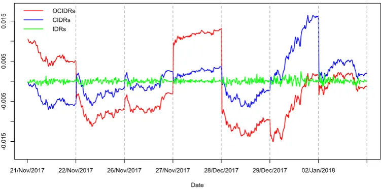
obtain the IDRs, we usew = 1to produce the 5-min intra-day log returns. Figure 5.1 shows these three types of intra-day curves across seven days. The stationarity of all three return

curves is examined by using the stationary tests proposed by Horváthet al. (2014). The results

suggest that all intra-day return series are stationary.

We begin by testing for functional conditional heteroscedasticity for each curve type. The

results of these tests are given in Table 5.1, which suggest that each sample of curves exhibit

strong conditional heteroscedasticity.

A natural next step is to posit and evaluate models to capture this conditional heteroscedasticity.

For this we consider two models: standard scalar GARCH models and FGARCH models. The

motivation for considering standard scalar GARCH models for this purpose is that we might

at first expect that the volatility in each of these curves can be adequately accounted for by

scaling each curve by the conditional standard deviation through the fitting of a GARCH model

to the end-of-day returns, i.e. a large magnitude of the return on the previous day spells high

Figure 5.1. Seven days of Intra-day return curves from S&P 500

-0

.0

1

5

-0

.0

0

5

0.005

0.015

Date

21/Nov/2017 22/Nov/2017 26/Nov/2017 27/Nov/2017 28/Dec/2017 29/Dec/2017 02/Jan/2018 OCIDRs

CIDRs

IDRs

asxi = log(Pi(1))−log(Pi−1(1)),1 ≤i ≤500, to which we fit a scalar GARCH(p,q) model

by using a quasi maximum likelihood estimation approach. The orders _{p, q}are selected as the minimum orders for which the estimated residualsεˆi =xi/σˆi are plausibly a strong white noise as measured by the Li-Mak test; see Li and Mak (1994), resulting in the selection of a

GARCH(1,1) model, as shown in Panel A in Table 5.2.

We then apply the proposed tests for conditional heteroscedasticity to the fitted residuals

func-tions of intra-day returns

˜

εi(t) = Xi(t)/σˆi.

The results of these tests are given in Panel B in Table 5.2, which show that these curves still

exhibit a substantial amount of conditional heteroscedasticity.

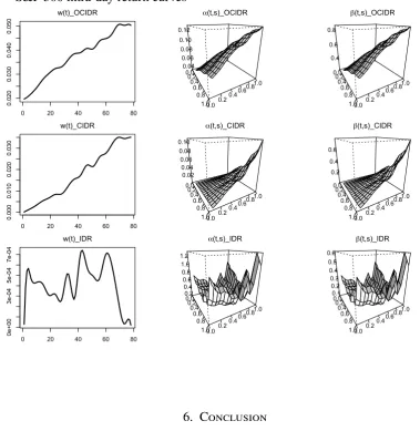
Next, we consider the FARCH(1) and FGARCH(1,1) models for these curves. We fit each

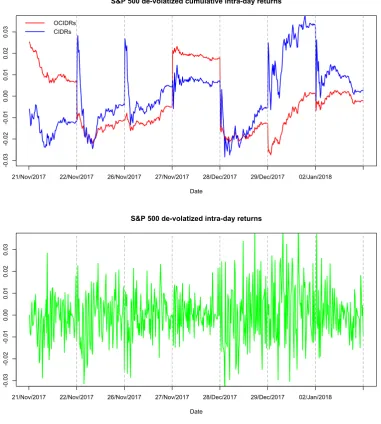
model withL= 1in (3.1) in order to be consistent with the simulation section, and evaluate the adequacy of each model as proposed above. Figure 5.2 shows plots ofw(t)and wire-frame plots of the kernelsα(t, s)andβ(t, s)for the FGARCH(1,1) model for each type of intra-day return curve. We then estimateσˆi(t)recursively with the initial values of wˆ(t), and the de-volatized intra-day returnεˆi(t)is fitted per Equation (3.3). Figure 5.3 exhibits the de-volatized intra-day returns over seven days by using the FGARCH(1,1) model.

Table 5.3 reports the p-values from the diagnostic checks of the FGARCH(1,1) and FARCH(1)

models applied to de-volatized intra-day returns. All of the three diagnostic tests show broadly

consistent results at specified significance levels. The FARCH(1) model is generally deemed to

be inadequate for each curve type, although this model performs as we expected to adequately

model conditional heteroscedasticity at lag 1. By contrast, the P values in Panel B of Table

5.3 suggest that the FGARCH(1,1) model is generally acceptable for modelling the conditional

heteroscedasticity of all three curve types. In conjunction with the above results showing that

these curves cannot be adequately de-volatized simply by scaling with the conditional standard

deviation estimates from GARCH models for the scalar returns, we draw the following tentative

conclusions from this analysis: 1) the magnitude of the return cannot fully explain the volatility

of intraday prices observed on subsequent days; instead we should consider the entire path

of the price curve on previous days in order to adequately model future intra-day conditional

heteroscedasticity, and 2) the FGARCH class of models seems to be effective for modeling

intra-day conditional heteroscedasticity.

Table 5.1. Heteroscedasticity tests on the intra-day returns of S&P 500

K=1 K=5 K=10 K=20

Stats P value Stats P value Stats P value Stats P value

OCIDRs VN,K 6.94 0.01 52.69 0.00 73.70 0.00 76.20 0.00

M_N,K 1.19 0.00 8.44 0.00 12.08 0.00 12.82 0.00

CIDRs _MVN,K 8.73 0.00 36.11 0.00 37.76 0.00 49.35 0.00

N,K 0.06 0.00 0.26 0.00 0.29 0.00 0.42 0.00

IDRs VN,K 189.87 0.00 437.99 0.00 461.05 0.00 481.15 0.00

M_{N,K 4.73e-08 0.00 1.25e-07 0.00 1.55e-07 0.00 2.30e-07 0.00}

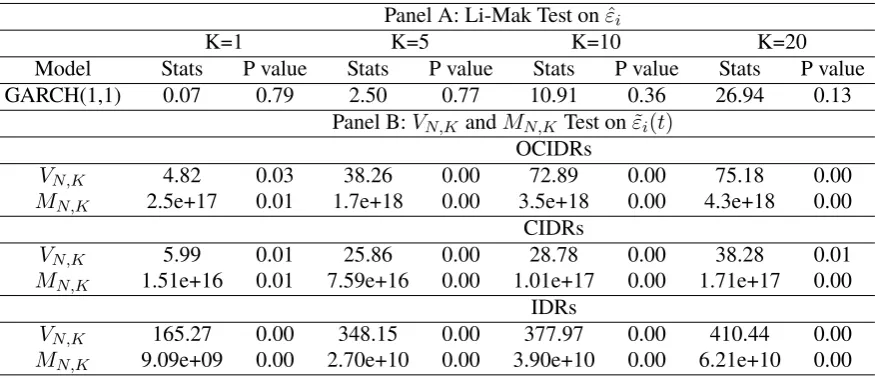
Table 5.2. Heteroscedasticity tests of de-volatized return curves ε˜i(t) using a GARCH(p,q) model

Panel A: Li-Mak Test onεˆ_i

K=1 K=5 K=10 K=20

Model Stats P value Stats P value Stats P value Stats P value GARCH(1,1) 0.07 0.79 2.50 0.77 10.91 0.36 26.94 0.13

Panel B:V_N,KandM_{N,KTest on}ε_˜i(t₎

OCIDRs

V_{N,K 4.82 0.03 38.26 0.00 72.89 0.00 75.18 0.00} M_{N,K 2.5e+17 0.01 1.7e+18 0.00 3.5e+18 0.00 4.3e+18 0.00}

CIDRs

V_{N,K 5.99 0.01 25.86 0.00 28.78 0.00 38.28 0.01} M_{N,K 1.51e+16 0.01 7.59e+16 0.00 1.01e+17 0.00 1.71e+17 0.00}

IDRs

Figure 5.2. Plots of the estimated kernels for the FGARCH(1,1) model for the S&P 500 intra-day return curves

0 20 40 60 80

0.020 0.030 0.040 0.050 w(t)_OCIDR 0.0 0.2 0.4 0.6 0.8 1.00.0 0.2 0.40.6 0.81.0 0.04 0.06 0.08 0.10 0.12 α(t,s)_OCIDR 0.0 0.2 0.4 0.6 0.8 1.00.0 0.2 0.40.6 0.81.0 0.4 0.6 0.8 β(t,s)_OCIDR

0 20 40 60 80

0.000 0.010 0.020 0.030 w(t)_CIDR 0.0 0.2 0.4 0.6 0.8 1.00.0 0.2 0.40.6 0.81.0 0.02 0.04 0.06 0.08 0.10 α(t,s)_CIDR 0.0 0.2 0.4 0.6 0.8 1.00.0 0.2 0.40.6 0.81.0 0.2 0.4 0.6 β(t,s)_CIDR

0 20 40 60 80

0 e +0 0 3 e -0 4 5 e -0 4 7 e -0 4 w(t)_IDR 0.0 0.2 0.4 0.6 0.8 1.00.0 0.20.4 0.60.8 1.0 0.2 0.4 0.6 0.8 1.0 1.2 α(t,s)_IDR 0.0 0.2 0.4 0.6 0.8 1.00.0 0.20.4 0.60.8 1.0 0.1 0.2 0.3 0.4 0.5 0.6 β(t,s)_IDR 6. Conclusion

We proposed two portmanteau-type conditional heteroscedasticity tests for functional time

series. By applying the test statistics to model residuals from the fitted functional GARCH

models, our tests also provide two heuristic and one asymptotically valid goodness-of-fit test for

such models. Simulation results presented in this paper show that both tests have good size and

power to detect conditional heteroscedasticity in functional financial time series and assess the

goodness-of-fit of the FGARCH models in finite samples. In an application to the dense intraday

price data, we investigated the conditional heteroscedasticity of three types of the intra-day return

curves, including the overnight cumulative intra-day returns, the cumulative intra-day returns

and the intra-day log returns from two assets. Our results suggested that these curves exhibit

substantial evidence of conditional heteroscedasticity that cannot be accounted for simply by

rescaling the curves by using measurements of the conditional standard deviation based on the

magnitude of the scalar returns. However, the functional conditional volatility models often

Figure 5.3. Plots of de-volatized S&P 500 intra-day return curves based on an FGARCH(1,1) Model

-0

.0

3

-0

.0

2

-0

.0

1

0.00

0.01

0.02

0.03

S&P 500 de-volatized cumulative intra-day returns

Date

21/Nov/2017 22/Nov/2017 26/Nov/2017 27/Nov/2017 28/Dec/2017 29/Dec/2017 02/Jan/2018 OCIDRs

CIDRs

-0

.0

3

-0

.0

2

-0

.0

1

0.00

0.01

0.02

0.03

S&P 500 de-volatized intra-day returns

Date

21/Nov/2017 22/Nov/2017 26/Nov/2017 27/Nov/2017 28/Dec/2017 29/Dec/2017 02/Jan/2018

appeared to be adequate for modeling this observed functional conditional heteroscedasticity in

financial data.

Appendix A. Proofs of results in Sections 2

Proofs of Theorem 2.1. First we show (2.5). Under_H0and Assumption 2.1 the random variables

Y1,i = kXik2 are independent and identically distributed, and satisfy EY14,i < ∞. (2.5) now follows Theorem 7.2.1 and problem 2.19 of Brockwell and Davis (1991).

In order to show (2.6), we recall some notation and the statement of Lemma 5 in Kokoszkaet

Table 5.3. Diagnostic tests of FGARCH(1,1) and FARCH(1) models applied to the S&P 500 return curves.

Panel A: FARCH(1)

Stats P value Stats P value Stats P value Stats P value

OCIDRs

Vheuristic

N,K,ε 0.26 0.61 33.94 0.00 50.07 0.00 52.53 0.00

Mheuristic

N,K,ε 5.86 0.52 216.08 0.00 324.45 0.00 358.37 0.00

M_{N,K,ε 5.86 0.43 216.08 0.00 324.45 0.00 358.37 0.00}

CIDRs

Vheuristic

N,K,ε 2.40 0.12 33.11 0.00 36.59 0.00 52.32 0.00

Mheuristic

N,K,ε 66.07 0.05 586.09 0.00 737.63 0.00 1264.67 0.00

M_{N,K,ε 66.07 0.14 586.09 0.00 737.63 0.00 1264.67 0.00}

IDRs

Vheuristic

N,K,ε 1.16 0.28 20.84 0.00 26.02 0.00 45.91 0.00

Mheuristic

N,K,ε 120.50 1.00 2942.47 0.34 4299.53 0.97 9407.58 0.96

M_{N,K,ε 120.50 0.98 2942.47 0.00 4299.53 0.00 9407.58 0.00}

Panel B: FGARCH(1,1)

K=1 K=5 K=10 K=20

Stats P value Stats P value Stats P value Stats P value

OCIDRs

Vheuristic

N,K,ε 0.11 0.74 2.15 0.83 5.80 0.83 8.88 0.98

Mheuristic

N,K,ε 5.11 0.59 27.36 0.84 65.30 0.85 106.47 0.99

M_{N,K,ε 5.11 1.00 27.36 1.00 65.30 1.00 106.47 1.00}

CIDRs

Vheuristic

N,K,ε 0.17 0.68 4.00 0.55 8.55 0.58 18.40 0.56

Mheuristic

N,K,ε 25.01 0.87 232.20 0.59 469.33 0.61 923.36 0.72

M_{N,K,ε 25.01 1.00 232.20 1.00 469.33 1.00 923.36 1.00}

IDRs

Vheuristic

N,K,ε 3.95 0.05 11.54 0.04 16.77 0.08 33.25 0.03

Mheuristic

N,K,ε 301.90 1.00 3912.94 1.00 7170.58 1.00 17859.05 1.00

M_{N,K,ε 301.90 0.99 3912.94 0.63 7170.58 0.91 17859.05 0.16}

of functionsf : [0,1]2 _→RK_{, mapping the unit square to the space ofK-dimensional column} vectors with real entries, satisfying

Z Z

{f(t, s)_}⊤f(t, s)dtds <_∞.

This space is a separable Hilbert space when equipped with the inner product

hf, giG,1 =

Z Z

{f(t, s)}⊤g(t, s)dtds.

Let_k·kG,1denote the norm induced by this inner product. Leth·,·iFdenote the matrix Frobenius

inner product, and let _{k · k}F denote the corresponding norm; see Chapter 5 of Meyer (2000).

Further let _G2 denote the space of functions f : [0,1]4 → RK×K, equipped with the inner

product

hf, giG,2 =

Z Z Z Z

hf(t, s, u, v), g(t, s, u, v)iFdtdsdudv.

for which _hf, f_iG,2 < ∞. G2 is also a separable Hilbert space when equipped with this inner

product.

Let ψK : [0,1]4 → RK×K be a matrix valued kernel where the 1 ≤ i, j ≤ K component is denoted byψK,i,j(t, s, u, v). We then defineψKby

(A.1) ψK,i,j(t, s, u, v) =

   

  

cov(X02(t), X02(u))cov(X02(s), X02(v)), 1≤i=j ≤K.

0 1_≤i₆=j _≤K.

The kernelψK defines a linear operatorΨK :G1 → G1 by

ΨK(f)(t, s) =

Z Z

ψK(t, s, u, v)f(u, v)dudv, (A.2)

where the integration is carried out coordinate-wise. Following the preamble to the proof of

Lemma 5 of Kokoszka et al. (2017), it follows that the operator ΨK is compact, symmetric,

and positive definite. Due to these three properties, we have by the spectral theorem for positive

definite, self-adjoint, compact operators, e.g. Chapter 6.2 of Riesz and Nagy (1990), thatΨK

defines a nonnegative and decreasing sequence of eigenvalues and a corresponding orthonormal

basis of eigenfunctionsϕi,K(t, s),1≤i <∞, satisfying

ΨK(ϕi,K)(t, s) =ξi,Kϕi,K(t, s), with ∞

X

i=1

ξi,K <∞. (A.3)

With this notation, we now define

ˆ

ΓN,K(t, s) =

√

N{ˆγ1(t, s), . . . ,γˆK(t, s)}⊤ ∈ G1.

Under _H0 and Assumption 2.1, the sequence {Xi2(t)} satisfies the conditions of Lemma 5 of Kokoszka et al. (2017), which implies that ΓˆN,K(t, s)

D(G1)

→ ΓK(t, s), where ΓK(t, s) is a Gaussian process with covariance operatorΨK, and

D(G1)

→ denotes weak convergence in_G1. It

now follows from the Karhunen-Loéve representation and continuous mapping theorem that

MN,K =kΓˆN,Kk2 D

→ kΓKk2 D

=

∞

X

i=1

A simple calculation based on (A.1) shows that the eigenvalues of ΨK are products of the

eigenvalues defined by (2.4),_{λiλj, 1≤ i, j < ∞}, with each eigenvalue having multiplicity

K, giving the form of the limit distribution in (2.6).

Justification of (4.2). Using proposition 5.10.16 of Bogachev (1998), we have that

E(_kΓKk2H,1) =tr(ΨK) = K

Z

cov(X₀2(t), X₀2(t))dt

2

,

and

var(_kΓKk2H,1) = 2tr(Ψ2K) = 2K

Z Z

cov(X2

0(t), X02(s))dtds

2

.

Proof of Theorem 2.2. We only show (2.7) as (2.8) follows similarly from it. Let Ch(t, s) = cov(X2

i(t), Xi2+h(s))6= 0. It follows from the assumedL8-m-approximability ofXi thatXi2 is

L4_{-m-approximable, from which we can show that}

kγˆh(t, s)−Ch(t, s)k=OP(1/

√

N).

Now MN,K ≥ Nkγˆh(t, s)k2, and kγˆh(t, s)k2 = kγˆh −Chk2 + 2hγˆh −Ch, Chi+kChk2. It follows thatN[kγˆh −Chk2+ 2hγˆh −Ch, Chi] = OP(

√

N), andNkChk2 diverges to positive

infinity at rateN, yielding the desired result.

Proof of Theorem 2.3. Again we only prove (2.10) as (2.9) follows from it by a similar argument.

By squaring both sides of of (2.1) and iterating (2.2), we obtain that

X2

i(t) =ωα(t) + ∞

X

ℓ=0

α(ℓ)(Vi−ℓ)(t),

where the series on the right hand side of the above equation converges inL2_[0,1]with

proba-bility one, and

ωα(t) = ∞

X

ℓ=0

α(ℓ)(ω)(t).

Therefore,X2

i(t)is a linear process inL2[0,1]with meanωα(t)generated by the weak functional white noise innovationsVias defined in Bosq (2000). It now follows from Assumption 2.1 and

the ergodic theorem that

ˆ

γh(t, s)− ∞

X

j=0

Eα(j)(Vj)(t)α(j+h)(Vj)(s)

=oP(1).

It follows from this and the reverse triangle inequality that

MN,K

N =

K

X

h=1

kˆγhk2 p

→

K

X

h=1

∞

X

j=0

Eα(j)(Vj)(t)α(j+h)(Vj)(s)

2

,

as desired.

Appendix B. Proof of Theorem 3.1 and estimation of parameters/kernels

in Section 3.1

We first develop some notation and detail the assumptions that we use to establish Theorem 3.1.

Recall from equation (3.2) that the FGARCH equations along with (3.1) imply that

s2

i =D+Ax2i−1+Bs2i−1

wherex2

i = [hXi2(t), φ1(t)i, . . . ,hXi2(t), φL(t)i]⊤, s2i = [hσi2(t), φ1(t)i, . . . ,hσ2i(t), φL(t)i]⊤, the coefficient vectorD= [d1, . . . , dL]⊤ ∈RL, and the coefficient matricesAandB areRL×L with(j, j′_{)entries bya}

j,j′ andb_j,j′, respectively. LetΓ₀(t, s) = α(t, s)ε2₀(s) +β(t, s). We make

the following assumptions:

Assumption B.1. E R

Γ0(·, s)ds

2

∞ <1, andω ∈C[0,1].

Assumption B.2. Q0 is nonsingular.

Assumption B.3. x2

0is not measurable with respect toF0.

Assumption B.4. infθ∈Θ|det(A)| > 0 and supθ∈ΘkBkop < 1, where k · kop is the matrix

operator norm ofB.

Assumption B.5. E_kε4

0k∞ <∞

Assumptions B.1–B.4 come directly from Aue et al. (2017), and imply both that there exists

a strictly stationary and causal solution to the FGARCH equations inC[0,1], and thatθˆN is a strongly consistent estimator ofθ0 that also satisfies the central limit theorem. Assumption B.5

appears in Cerovecki et al. (2019), and is a somewhat stronger assumption than that of Theorem

3.2 of Aue et al (2018). It is used in the proofs below mainly to establish uniform integrability

of terms of the form_kXi/σik∞. Assumption B.6 is implied by the conditions of Cerovecki et al. (2019) that the functionsφi are strictly positive and thatD∈ ΘD ⊂(0,∞)L, whereΘD is compact, but also may hold under more general conditions.

Theorem B.1(Precise statement of Theorem 3.1:). LetΓ_N,K(ε,θ) = (√Nˆγε,1, ...,

√

Nγˆε,K)⊤ ∈ G1.

Then under Assumption B.1–B.6,

Γ(_N,Kε,θ) D(G1)

→ Γε,θ,

whereΓε,θ is a mean zero Gaussian process inG1 with covariance operatorsΨ(Kε,θ)defined by

Ψ(_Kε,θ)(f)(t, s) =

Z Z

ψ_K(ε,θ)(t, s, u, v)f(u, v)dudv,

(B.1)

whereψ_K(ε,θ)(t, s, u, v)is a matrix valued kernel defined by(3.8). In addition,

MN,K,ε →D ∞

X

i=1

ξi,Kχ21(i),

whereξi,K i≥1are the eigenvalues ofΨ(Kε,θ).

Before proving this result, we introduce further notation. We write σ2

i(t, θ) to indicate the dependence ofσ2

i(t)on the vector of parametersθ, and similarly write

s2

i(θ) = [hσ2i(t, θ), φ1(t)i, . . . ,hσ2i(t, θ), φL(t)i]⊤. It follows that withΦ(t) = (φ1(t), ..., φL(t))⊤,

σ2_i(t, θ) = s2

i(θ)⊤Φ(t). Iterating (3.2), we see using Assumption (B.4) that

σ2_i(t, θ) =

∞

X

ℓ=0

Bℓξi−ℓ

!⊤

Φ_{(t), whereξi−ℓ =D+A}x2

i−1−ℓ. (B.2)

We define

˜

σ_i2(t, θ) =

i−1

X

ℓ=0

Bℓξℓ

!⊤ Φ_(t),

(B.3)

which allows us to define

ˆ

σ_i2(t) = ˜σ2_i(t,θˆN). (B.4)

In addition toγˆε,hdefined in (3.4), we also define

˜

γε,h(t, s, θ) =

1

N

N−h

X

i=1

X2

i(t)

˜

σ2

i(t, θ)−

1 X

2

i+h(s)

˜

σ2

i+h(s, θ)

−1

.

(B.5)

and

γ⋆_ε,h(t, s, θ) = 1

N

N−h

X

i=1

X2

i(t)

σ2

i(t, θ)

−1 X

2

i+h(s)

σ2

i+h(s, θ)

−1

,

(B.6)

so thatˆγε,h(t, s) = ˜γε,h(t, s,θˆN). Below we letθ(j)denote thej′th coordinate ofθ.

Lemma B.1. Under Assumptions B.1–B.6, for allhsuch that1_≤h_≤K,

sup

θ∈Θ

√

Nkγ˜ε,h(·,·, θ)−γε,h⋆ (·,·, θ)k=oP(1), (B.7)

and

max

j∈{1,...,L+2L2

}supθ∈Θ

∂˜γε,h(·,·, θ)

∂θ(j) −

∂γ⋆

ε,h(·,·, θ)

∂θ(j)