Munich Personal RePEc Archive
Trade Liberalization, Technology
Diffusion, and Productivity
Kishi, Keiichi and Okada, Keisuke
Kansai University
August 2018
Online at
https://mpra.ub.uni-muenchen.de/88597/
Trade Liberalization, Technology Diffusion, and Productivity
∗Keiichi Kishi† Keisuke Okada‡
August 22, 2018
Abstract
This study develops the international trade theory of technology diffusion with heterogeneous firms. Each new entrant randomly searches for and meets incumbents and then adopts their existing tech-nology. As in previous international trade models based on firm heterogeneity, trade liberalization induces the least productive firms to exit, and then the resources can be reallocated toward more productive firms. However, we show that this resource reallocation effect is mitigated by the entry of low-productive firms. Trade liberalization facilitates the diffusion of existing low-productive technolo-gies to new entrants, which shifts the weight in the productivity distribution from the upper tail area to the area around the least productivity. Thus, some resources can be reallocated toward low-productive firms. In addition, trade liberalization reduces domestically produced varieties. Consequently, we show the non-monotonic relationship between trade liberalization and aggregate productivity.
JEL classification: F12, L11, O33
Keywords: International trade, Innovation, Productivity distribution
∗The authors would like to thank Yoshiyasu Ono, Tadashi Morita, Masashi Tanaka, and the seminar participants at
Kansai University and Osaka University for their valuable comments. This work received financial support from the JSPS KAKENHI Grant Numbers JP15H03354, JP16H02026, and JP17K13740. We are responsible for any remaining errors.
†Faculty of Economics, Kansai University, 3-3-35 Yamate-cho, Suita-shi, Osaka 564-8680, Japan, E-mail address:
‡Faculty of Economics, Kansai University, 3-3-35 Yamate-cho, Suita-shi, Osaka 564-8680, Japan, E-mail address:
1
Introduction
Trade liberalization has been a central issue in international economics and the costs and benefits of globalization have been an interesting subject for economists and policymakers. International trade models with heterogeneous firms such as those proposed by Melitz (2003) and Melitz and Ottaviano (2008) show that trade liberalization causes low-productive firms to exit because of intense market selection. As a consequence, resources reallocate to high-productive firms under the so-called “resource reallocation effect,” which contributes to increasing aggregate productivity at the industry level. Many empirical studies confirm the resource reallocation effect (or market selection effect) caused by trade liberalization. Based on the foregoing, this study investigates the effects of trade liberalization on productivity, considering the entry and exit of firms. Because the entry and exit of firms occur constantly, it is important to consider what kinds of firms contribute to the productivity gain. Aggregate productivity is affected not only by the market shares of surviving firms but also by the entry and exit of firms. By proposing a new method of productivity decomposition based on Olley and Pakes (1996), Melitz and Polanec (2015) show that the contribution of entering firms in Slovenian manufacturing sectors after economic reforms (e.g., the liberalization of prices and wages, deregulation of firm entry, and privatization of state-owned firms) is overvalued compared with that in previous studies. Specifically, among surviving, entering, and exiting firms, the contribution of entering firms to labor productivity is negative and the contribution to total factor productivity is nil. This result indicates that new entrant firms, which tend to be small and therefore most likely to leave the market (World Trade Organization, 2016), do not necessarily have high productivity after economic reforms. In this study, we refer to this as the “low-productive entrant effect.” By considering this low-productive entrant effect explicitly, we examine how trade liberalization af-fects productivity. In the international trade model presented herein, constructed based on the model of Melitz (2003) with technology diffusion ´a la Aghion and Howitt (1998, Ch. 3), Lucas and Moll (2014), and Perla and Tonetti (2014), trade liberalization causes both the resource reallocation effect (owing to the market selection effect) and the low-productive entrant effect. Each new entrant randomly searches for and meets an incumbent and then learns its existing technology. Some new entrants succeed in adopting the frontier (the most productive) technology, as in Aghion and Howitt (1998, Ch. 3). The other new entrants adopt existing non-frontier technologies, as in Lucas and Moll (2014) and Perla and Tonetti (2014). Then, the model generates theendogenous stationary Pareto productivity distribution.1 Therefore, trade liberalization changes the shape (Pareto exponent) of the distribution. Specifically, we show that trade liberalization increases the Pareto exponent because of the low-productive entrant effect. That is, trade liberalization induces the entry of low-productive firms, which shifts the weight in the productivity distribution from the upper tail area to the area around the least productivity (minimum support of the distribution). Therefore, the endogenous response of the distribution has a negative effect on aggregate productivity. On the contrary, as in the Melitz (2003) model, trade liberalization induces the least productive firms to exit the market, which causes the reallocation of resources to high-productive
1
firms, thereby affecting aggregate productivity positively. In summary, the resource reallocation effect is mitigated by the low-productive entrant effect. In other words, some resources are reallocated toward low-productive new entrants. Further, as shown in the Melitz (2003) model, trade liberalization reduces the number of domestic varieties, which also has a negative effect on aggregate productivity. Then, the net effect of trade liberalization on aggregate productivity depends on whether the resource realloca-tion effect dominates the low-productive entrant effect and the reducrealloca-tion in domestic varieties. Indeed, we numerically demonstrate the non-monotonic relationship between trade liberalization and aggregate productivity.
The low-productive entrant effect also worsens welfare because of the negative effect on aggregate productivity. However, we numerically show that trade liberalization increases welfare in the steady-state level. In the model, real income is the welfare measure in the steady state. Then, two competing effects on real income exist. First, trade liberalization reduces the ideal price index because of the dominant resource reallocation effect and the increase in the share of imported varieties, which has a positive effect on real income. Second, trade liberalization may reduce average assets per capita because of the low-productive entrant effect and reduction in domestic varieties. Then, trade liberalization reduces asset income, which has a negative effect on real income. Consequently, we numerically show that the effect of the reduction in the price index on real income dominates the reduction in asset income and thus trade liberalization increases real income and welfare in the steady-state level.
which to generate an endogenous Pareto exponent. Then, we can analytically clarify the impact of trade liberalization on the distribution through the entry of low-productive firms. By virtue of the endogenous distribution, this study thus incorporates not only the effect of exiting firms on productivity but also the effect of entering firms on productivity.
An extensive body of empirical research has examined the relationship between trade liberalization and productivity both in developed and in developing countries. Studies of developed countries include Bernard et al. (2003) and Bernard et al. (2006) for the United States and Trefler (2004), Lileeva (2008), and Lileeva and Trefler (2010) for Canada. Other studies targeting developing countries include Pavcnik (2002) for Chile, Amiti and Konings (2007) for Indonesia, Fernandes (2007) for Colombia, Goldberg et al. (2010), Nataraj (2011), and Topalova and Khandelwal (2011) for India, Bustos (2011) for Argentina, and Yu (2015) for China.
Most of these studies confirm that trade liberalization increases productivity monotonically at the industry and firm (or plant) levels. There are likely to be two channels through which trade liberalization increases productivity. One is the reallocation of resources from low-productive sectors to high-productive ones as the Melitz (2003) model predicts. Empirical studies such as Pavcnik (2002) and Bernard et al. (2006) support this view. Bernard et al. (2006), for example, use data on U.S. manufacturing industries and plants from 1977 to 2001 to examine the effects of industry-level tariffs and transportation costs. They find that a reduction in trade costs increases industry productivity and that these gains are attributed to the reallocation to high-productive plants within industries. The other is the adoption of more advanced technologies. Bustos (2011) uses data on Argentinean firms and finds that a regional free trade agreement (FTA), MERCOSUR, induces firms to increase investment in technology.23
Although, to the best of our knowledge, no studies explicitly examine the non-monotonic relationship between trade liberalization and productivity, some studies imply such a relationship. Trefler (2004) examines the effects of the Canada-U.S. FTA on the labor productivity of Canadian manufacturing at the industry and plant levels. He shows that U.S. tariff concessions do not have a significant impact on labor productivity at the industry level, although they significantly increase labor productivity at the plant level.4 As a reason for this result, he points out that U.S. tariff concessions may promote the entry
of less productive plants. In this study, we use Trefler’s (2004) dataset and confirm the negative impact of trade liberalization on labor productivity in certain circumstances, as our model predicts.
The contributions of this study to existing research are summarized as follows. First, by incorporating the process of technology diffusion, we derive the endogenous stationary Pareto productivity distribution. Second, we show that trade liberalization changes the shape (Pareto exponent) of the distribution, which is consistent with the low-productive entrant effect through trade liberalization. Finally, we quantitatively
2
Yeaple (2005), Ederington and McCalman (2008), Lileeva and Trefler (2010), and Bustos (2011) theoretically show that trade liberalization induces some firms to invest in new technologies, which increases plant-level productivity.
3
Recently, empirical studies have paid attention to tariff reductions in final goods and imported intermediate goods as measures of trade liberalization. On the one hand, lowering output tariffs leads to competition, which raises firms’ productivity. On the other hand, reductions in input tariffs cause firms to increase efficiency because they can obtain cheaper imported inputs. Most studies show that both input and output tariff reductions have a positive impact on productivity at the firm level (e.g., Amiti and Konings, 2007; Nataraj, 2011; Topalova and Khandelwal, 2011; Yu, 2015).
4
assess the net effect of trade liberalization on aggregate productivity that consists of the resource real-location effect, low-productive entrant effect, and reduction in domestic varieties. Then, we numerically demonstrate the non-monotonic relationship between trade liberalization and aggregate productivity.
The remainder of the paper is organized as follows. In Section 2, we outline the trade model of Melitz (2003) with technology diffusion `a la Aghion and Howitt (1998, Ch. 3), Lucas and Moll (2014), and Perla and Tonetti (2014). In Section 3, we derive the productivity distribution across active firms to yield average productivity. In Section 4, we analytically show the impact of trade liberalization on average productivity. In Section 5, we numerically investigate the impact of trade liberalization on average and aggregate productivities as well as welfare. Section 6 revisits Trefler’s (2004) study and confirms the negative effect of trade liberalization in certain circumstances. Section 7 concludes.
2
Theoretical framework
We develop an international trade model based on technology diffusion. There are 1 +N symmetric countries. When N = 0, the model describes an autarkic economy, whereas when N > 0, the model describes an open economy. Time is continuous. We focus on the balanced-growth equilibrium in which all endogenous variables grow at constant rates. We omit the country index when representing the country’s variables since we focus on symmetric countries.
2.1 Household
There is a representative household with the following utility:
U =
∫ ∞
0
e−ρtLc(t)
1−θ−1
1−θ dt, (1)
where ρ > 0 is the subjective discount rate, θ > 0 is the inverse of the intertemporal elasticity of substitution,c(t) denotes consumption per capita at timet, andLis the population size, which is constant over time. Hereafter, we omit time twhenever no ambiguity results.
The household’s budget constraint expressed in per capita terms is
˙
a= 1 +ra−P c, (2)
where a is the value of assets per capita, 1 represents the wage rate, which is normalized to unity (i.e., we take labor as the num´eraire),r is the interest rate, and P is the price of the consumption good.
The representative household’s optimization problem implies the well-known Euler equation for con-sumption:
˙
c c =
1
θ
(
r−ρ−P˙
P
)
(3)
and the transversality condition:
lim
t→∞
e−ρtc−θa
According to Eq. (2), the growth rates of both a and P c must be zero in the balanced-growth equilibrium:
0 = a˙
a =
˙
P
P +
˙
c
c. (5)
Then, the budget constraint (2) can be rewritten as
P c= 1 +ra. (6)
That is, expenditure P c for consumption equals the sum of wage income 1 and asset income ra in the balanced-growth equilibrium.
2.2 Final good
The final good is produced by using the continuum of intermediate goods under perfect competition, according to the following production function:
Q=
(∫
ω∈Ω
q(ω)σ−σ1dω
) σ σ−1
, (7)
where Q is the output of the final good, q(ω) is the intermediate input of variety ω ∈ Ω used in the production of the final good, Ω is the set of the varieties of the intermediate good available for the production of the final good in a typical country, andσ >1 is the elasticity of substitution between any two intermediate goods. The conditional factor demand function for q(ω) derived from Eq. (7) is
q(ω) = (
P p(ω)
)σ
Q, (8)
wherep(ω) is the price of the intermediate goodω and the price of the final good is
P =
(∫
ω∈Ω
p(ω)1−σdω
) 1 1−σ
. (9)
The final good can be used only for consumption, and thus its market-clearing condition is
Q=cL. (10)
2.3 Intermediate good
τ units of a good must be shipped for 1 unit to arrive in a foreign country. We omit the notation ω, as it is sufficient to identify each firm by its productivityφ.
Under Eq. (8), firms whose productivity is φ choose the domestic price to maximize the domestic profit. Then, the domestic profit for a firm whose productivity is φis given by
Πd(φ) = max
{ 0,
( 1
σ−1 ) (
σ−1
σ
)σ
φσ−1PσQ−f
}
. (11)
From Eq. (11), the exit cutoff productivity φ∗, where firms exit if and only ifφ < φ∗, is given by
Πd(φ∗) = 0 ⇐⇒ (φ∗)σ−1 = (σ−1)
(
σ σ−1
)σ(
f PσQ
)
. (12)
Similarly, firms whose productivity isφchoose the export price to maximize the export profit for a typical country. Then, the export profit for a firm whose productivity is φis given by
Πx(φ) = max
{ 0,
( 1
σ−1 ) (
σ−1
σ
)σ( 1
τ
)σ−1
φσ−1PσQ−fx
}
. (13)
From Eq. (13), threshold productivity φ∗x, where firms choose to export if and only if φ≥φ∗x, is given by
Πx(φ∗x) = 0 ⇐⇒ (φ∗x)
σ−1= (σ−1)( σ
σ−1 )σ
τσ−1
(
fx PσQ
)
. (14)
To simplify the analysis, define the log of relative productivity ϕ ≡ ln(φ/φ∗). Below, we simply
refer to ϕas either relative productivity or productivity whenever no ambiguity results. An active firm’s productivity φ is higher than exit cutoff φ∗; therefore, ϕ ≥ 0 holds for all active firms. Now, we can
rewrite the domestic profit (11) and export profit (13) by using ϕas follows:
πd(ϕ) =
f[e(σ−1)φ−1] forϕ≥0
0 otherwise (15)
πx(ϕ) =
(1
τ
)σ−1
f[e(σ−1)φ−e(σ−1)φ∗
x] for ϕ≥ϕ∗
x
0 otherwise, (16)
whereπd(ϕ)≡Πd(φ∗eφ),πx(ϕ)≡Πx(φ∗eφ), and
ϕ∗x ≡ln ( φ∗ x φ∗ ) = ( 1
σ−1 )
ln (
τσ−1fx
f
)
≥0. (17)
Now, we suppose that ϕ∗
x ≥ 0 ⇐⇒ τσ−1fx ≥ f holds, which ensures that the absolute export cutoff φ∗
x is larger than absolute exit cutoff φ∗ in the equilibrium. For convenience, we restate the following
Assumption 1 The iceberg cost and fixed cost of exporting a variety is sufficiently large:
τσ−1fx ≥f. (18)
Total profits for the firm whose productivity is ϕequal the sum of the domestic profit (15) and export profit (16) across all foreign markets:
π(ϕ)≡πd(ϕ) +N πx(ϕ). (19)
By using the definition of ϕ, we can derive the domestic price pd(ϕ) and the export price px(ϕ) as
follows:
pd(ϕ) = (
σ σ−1
) 1
eφφ∗ forϕ≥0 (20)
px(ϕ) = (
σ σ−1
)
τ
eφφ∗ forϕ≥ϕ ∗
x. (21)
Next, we derive the amount ld(ϕ) of labor required for production for the domestic market and the
amount lx(ϕ) of labor required for production for a foreign market as follows:
ld(ϕ) =
f[(σ−1)e(σ−1)φ+ 1] forϕ≥0
0 otherwise
(22)
lx(ϕ) =
(1
τ
)σ−1
f[(σ−1)e(σ−1)φ+e(σ−1)φ∗
x] forϕ≥ϕ∗
x
0 otherwise.
(23)
Then, total employment used for production by a firm with productivityϕis as follows:
l(ϕ)≡ld(ϕ) +N lx(ϕ). (24)
2.4 Frontier technology
The formation of the frontier technology follows Aghion and Howitt (1998, Ch. 3), Acemoglu et al. (2006), and Kishi (2016). Assume that a certain technology ¯φ(t) exists, whose initial value corresponds to the world frontier technology in the initial period, that is, ¯φ(0) = max{φ(ω)|ω ∈ ΩW(0)}, where
ΩW(0) represents the set of all the varieties of goods in the world (all countries) at time t = 0. Define g as the growth rate of the technology, that is, g ≡ φ˙¯(t)/φ¯(t), which is an exogenous variable. We can show that the technology coincides with the world frontier technology in all time periods, that is,
¯
φ(t) = max{φ(ω)|ω ∈ ΩW(t)} for all t ≥ 0, because later we show that some varieties ω always exist
whose technological level is ¯φ(t), and productivity φ(ω) cannot exceed ¯φ(t) for all t. It does not matter whether we define ¯φ as the domestic frontier technology or world frontier technology since we consider symmetric countries.
Defineµ(ϕ) as the stationary probability density function of an active firm’s log of relative productivity
the maximum support is ¯ϕ≡ln[ ¯φ(t)/φ∗(t)]. If the stationary distributionµ(ϕ) exists, the support of the
distribution must be constant over time. Therefore, the growth rate of φ∗(t) must be equal to that of
¯
φ(t) in the balanced-growth equilibrium, that is,g= ˙φ∗(t)/φ∗(t).
2.5 Technology diffusion and innovation
Innovations result from research and development (R&D) activity. By employing the fixed amountfe >0 of labor, a new entrant (R&D firm) produces one unit of a new intermediate product. The productivity of the new product is a random variable that takes either the frontier technology or the non-frontier technologies owned by existing firms. More precisely, as in Kishi (2016) and Benhabib et al. (2017), we consider the following R&D activities, which combine the elements of Aghion and Howitt (1998, Ch. 3), Lucas and Moll (2014), and Perla and Tonetti (2014). New entrants can attain frontier technology ¯φ
with exogenous probability p ∈ (0,1). This setup follows Aghion and Howitt (1998, Ch. 3). However, with probability 1−p, new entrants draw their productivity from the endogenous domestic productivity distribution µ(ϕ). This setup follows Lucas and Moll (2014) and Perla and Tonetti (2014). It does not matter whether new entrants draw their productivity from either the domestic or the global productivity distribution because we focus on symmetric countries.
In summary, each new entrant tries to improve its new product productivities (e.g., technological level, product management, product quality) by adopting the knowledge of existing firms. These knowledge adoptions (diffusions) create new products equipped with frontier knowledge with probabilityp. However, the knowledge adoptions are incomplete with probability 1−pin the sense that they create new products whose individual productivities are below the frontier.
2.6 Value of the firm and entry
Define the value of the firm with relative productivity ϕ as v(ϕ), which is the sum of discounted total profits (19). Given that firm exits form the market when productivity ϕ reaches the exit cutoff ϕ = 0, the value of the firm must follow the following Hamilton-Jacobi-Bellman (HJB) equation:5
rv(ϕ) =π(ϕ)−gv′(ϕ) for all ϕ >0, (25)
the value-matching condition
v(0) = 0, (26)
and the smooth-pasting condition
v′(0) = 0. (27)
The value-matching condition (26) ensures that the firm at the exit cutoff ϕ = 0 is indifferent between continuation, whose value isv(0), and exit, whose value is zero. According to Eqs. (15), (16), and (19), Eq. (25) at exit cutoff ϕ= 0 becomes rv(0) = −gv′(0). Then, to satisfy the value-matching condition (26), we require the additional condition v′(0) = 0, which is the smooth-pasting condition (27).6
5
The second term on the right-hand side of Eq. (25) represents the capital gaindv(φ)/dt=−gv′(φ).
6
Since total profits (19) are the sum of domestic profit πd(ϕ) and export profit N πx(ϕ) globally, the
value functionv(ϕ) can be written as
v(ϕ) =vd(ϕ) +N vx(ϕ), (28)
where vd(ϕ) is the sum of discounted domestic profits πd(ϕ) and vx(ϕ) is the sum of discounted export
profitsπx(ϕ). Then, vd(ϕ) must follow the following HJB equation:
rvd(ϕ) =πd(ϕ)−gv′d(ϕ) for all ϕ >0, (29)
the value-matching condition
vd(0) = 0, (30)
and the smooth-pasting condition
v′d(0) = 0. (31)
Given that each firm exports the product if and only if ϕ ≥ ϕ∗
x, vx(ϕ) must follow the following HJB
equation:
rvx(ϕ) =πx(ϕ)−gvx′(ϕ) for all ϕ > ϕ∗x, (32)
the value-matching condition
vx(ϕ∗x) = 0, (33)
and the smooth-pasting condition
v′x(ϕ∗x) = 0. (34)
According to Eq. (29), the boundary conditions (30) and (31), and the domestic profit (15), we obtain
vd(ϕ) = f e
(σ−1)φ r+ (σ−1)g −
f r + ( f r ) [
(σ−1)g r+ (σ−1)g
]
e−rT(φ), (35)
whereT(ϕ)≡ϕ/grepresents the waiting time until the firm with current productivityϕexits the domestic market. ϕ= (ϕ−0) of the numerator of T(ϕ) is the distance from current productivity ϕ to exit cutoff
ϕ= 0. On the contrary, gin the denominator ofT(ϕ) is the speed to run the given distance (ϕ−0). The sum of the first and second terms on the right-hand side of Eq. (35) represents the discounted value from the domestic market, in which firms continue to operate forever despite losses. Then, the third term is the additional value of the option to exit in the future. The option value decreases in ϕ and converges to zero asϕ→ ∞. This is because the exit option is invoked in the remote future when ϕbecomes very large, as captured by T(ϕ).
Similarly, according to Eq. (32), the boundary conditions (33) and (34), and the export profit (16), we obtain
vx(ϕ) = (
1
τ
)σ−1[
f e(σ−1)φ r+ (σ−1)g
]
−
( 1
τ
)σ−1
e(σ−1)φ∗x
( f r ) + ( 1 τ
)σ−1
e(σ−1)φ∗x
(
f r
) [
(σ−1)g r+ (σ−1)g
]
e−rTx(φ),
where Tx(ϕ) ≡ (ϕ−ϕ∗x)/g represents the waiting time until the firm with current productivity ϕ exits
the export market. (ϕ−ϕ∗
x) of the numerator of Tx(ϕ) is the distance from current productivity ϕ to
export cutoffϕ∗
x. On the contrary, g in the denominator of Tx(ϕ) is the speed to run the given distance
(ϕ−ϕ∗
x). Similarly, the sum of the first and second terms on the right-hand side of Eq. (36) represents
the discounted value from the foreign market, in which firms continue to export forever despite losses. Then, the third term is the additional value of the option to exit the export market in the future. The option value decreases in ϕ and converges to zero as ϕ→ ∞. This is because the exit option is invoked in the remote future whenϕ becomes very large, as captured byTx(ϕ).
We now derive the free-entry condition. Recall that each new entrant can produce one unit of a new variety of the good by using the fixed amount of labor fe > 0. New firms adopt frontier technology ¯ϕ
with exogenous probability p ∈ (0,1), while firms adopt the productivity drawn from the endogenous productivity distribution µ(ϕ) with probability 1−p. Then, if new firms enter the market, the following free-entry condition must hold:
fe=ve, (37)
where
ve ≡(1−p)
∫ φ¯ 0
v(ϕ)µ(ϕ)dϕ+pv( ¯ϕ). (38)
ve represents the expected benefit from entry. The first term on right-hand side of Eq. (38) represents the expected value from innovation ´a la Lucas and Moll (2014) and Perla and Tonetti (2014). The second term represents the expected value from innovation ´a la Aghion and Howitt (1998, Ch. 3).
2.7 Labor and asset markets
Define ¯M as the measure of Ω, which is the set of the available varieties of goods in a typical country,M
as the measure of the set of the varieties of domestic goods in a typical country, andMxas the measure of the set of the varieties of exported goods in a typical country. Then, the following equation holds because of the presence of symmetric countries:
¯
M =M +N Mx. (39)
That is, the total number ¯M of varieties used in a country is the sum of the number M of domestic varieties and the number N Mx of imported varieties.
The labor market-clearing condition is
L=M
∫ φ¯ 0
l(ϕ)µ(ϕ)dϕ+Mefe, (40)
whereMe represents the number of new entrants per unit of time. Then, according to Eqs. (39) and (40), given the lack of population growth, the following equation must hold in a balanced-growth equilibrium:
0 = M¯˙¯
M =
˙
M
M =
˙
Mx
Mx =
˙
Me
Me. (41)
the asset market-clearing condition requires the aggregate assets owned by the representative household to be equal to the aggregate equity value of all domestic firms:
aL=M
∫ φ¯ 0
v(ϕ)µ(ϕ)dϕ. (42)
Supposing either a closed or an open financial market is irrelevant because of the presence of symmetric countries.
3
Productivity distribution
In this section, we derive the endogenous productivity distribution of active firms. We then provide the economic intuitions behind the distribution.
3.1 Stationary productivity distribution
We derive the stationary productivity distribution µ(ϕ) for the log of relative productivity ϕ. We divide time into short intervals of duration ∆t >0, and theϕspace into short segments, each of length ∆h≡g∆t. Productivityϕfalls by ˙ϕ∆t=−g∆t≡ −∆hduring time interval ∆t. Define the entry rate of new entrants per unit of time as
ϵ≡ Me
M , (43)
which is constant over time in a balanced-growth equilibrium.
Now, consider the segment centered on ϕ ∈ (0,ϕ¯), which starts with the number M µ(ϕ, t)∆h of varieties at timet. In the next unit time period ∆t, all these varieties move to the left segment ϕ−∆h
because of the obsolescence of (reduction in) the log of relative productivity ϕ. New entrants as well as varieties from the right segment ϕ+ ∆h arrive to take their places ϕ. Therefore, the evolution of the productivity distribution is
M µ(ϕ, t)∆h=M µ(ϕ+ ∆h, t−∆t)∆h+ (1−p)Me∆tµ(ϕ, t−∆t)∆h, (44)
for allϕ∈(0,ϕ¯), whereµ(ϕ, t) represents the probability density function of the log of relative productivity
ϕat timet. The left-hand side of Eq. (44) represents the total number of varieties (located in segmentϕ
at time t), the first term on the right-hand side is the inflow of varieties into segmentϕat time tbecause of the obsolescence of the log of relative productivity, and the second term on the right-hand side is the inflow of varieties into segmentϕ at time tbecause of innovations. By canceling the common factor ∆h
in Eq. (44), dividing both sides by M, and noting that Eq. (43) holds, we yield
µ(ϕ, t) =µ(ϕ+ ∆h, t−∆t) + (1−p)ϵ∆tµ(ϕ, t−∆t). (45)
Expanding µ(ϕ+ ∆h, t−∆t) around µ(ϕ, t) following Taylor’s theorem yields
µ(ϕ+ ∆h, t−∆t) =µ(ϕ, t) +∂µ(ϕ, t)
∂ϕ ∆h−
∂µ(ϕ, t)
Higher-order terms of order such as (∆t)2 and (∆t)3 approach zero faster than ∆t, and thus these terms
are omitted from Eq. (46). Substituting Eq. (46) into Eq. (45), dividing both sides by ∆t, imposing ∆t→0, and simplifying yields the Kolmogorov forward equation (KFE):7
∂µ(ϕ, t)
∂t =g
∂µ(ϕ, t)
∂ϕ + (1−p)ϵµ(ϕ, t) for all ϕ∈(0,ϕ¯). (47)
In the stationary productivity distribution, ∂µ(ϕ, t)/∂t= 0 must hold. That is, the productivity distri-bution must be independent of timet. Then, the KFE (47) has the following stationary form:
0 =gµ′(ϕ) + (1−p)ϵµ(ϕ) for all ϕ∈(0,ϕ¯). (48)
We now derive the boundary conditions for the stationary distribution. First, consider the segment at ¯ϕ. The outflow from the varieties during time interval ∆t is M µ( ¯ϕ)∆h because of the obsolescence of relative productivity. The inflow of varieties into segment ¯ϕ during time interval ∆tis pMe∆t+ (1−
p)Me∆tµ( ¯ϕ)∆h because of innovations. In the stationary distribution, the inflow and outflow must be equal:
M µ( ¯ϕ)∆h=pMe∆t+ (1−p)Me∆tµ( ¯ϕ)∆h. (49)
Then, dividing both sides of Eq. (49) by M∆t, noting that Eq. (43) holds, imposing ∆t → 0, and simplifying yields
µ( ¯ϕ) = pϵ
g. (50)
Next, consider the boundary condition for the segment at exit cutoff ϕ= 0. Define δ∆t as the share of the varieties that reach exit cutoff ϕ= 0 during interval ∆t. That is, the following equation holds:
M δ∆t=M µ(∆h)∆h, (51)
where M δ∆t is the number of exiting firms, which equals the number M µ(0 + ∆h)∆h of firms located next to exit cutoffϕ= 0. Then, dividing both sides of Eq. (51) by ∆t, imposing ∆t→0, and simplifying yields
δ =µ(0)g. (52)
Finally, we derive the relationship between entry rate ϵand exit rateδ in a balanced-growth equilib-rium. According to Eq. (41), the number M of varieties is constant over time. Then, the inflow of new entrants and outflow of incumbents must be equal:
Me∆t=δM∆t, (53)
where the left-hand side represents the inflow of new entrants during time interval ∆tand the right-hand side represents the outflow of incumbents (the number of exiting firms) during time interval ∆t. Then,
7
by dividing both sides of Eq. (53) byM∆t, according to Eq. (43), we obtain
ϵ=δ. (54)
That is, entry rateϵis equal to exit rate δ in the balanced-growth equilibrium.
By solving the ordinary differential equation (48) by imposing the condition 1 =∫0φ¯µ(ϕ)dϕand noting Eqs. (52) and (54), we obtain the following lemma.
Lemma 1 The following equations describe the stationary distribution of the log of relative productivity
ϕ:
µ(ϕ) = (
η
1−p
)
e−ηφ for ϕ∈[0,ϕ¯], (55)
where
η ≡ (1−p)ϵ
g >0 and (56)
¯
ϕ =
( 1
η
) ln
( 1
p
)
>0. (57)
Lemma 1 implies thatµ( ¯ϕ) = lim
φ↑φ¯µ(ϕ). Then, the continuity at ¯ϕholds in the stationary distribution, µ(ϕ). That is, we can show that the stationary distribution (55) satisfies the boundary condition (50), even though we do not impose the condition (50) to solve the differential equation (48).
Lemma 1 shows that relative productivity ϕ follows the exponential distribution with the bounded support. This finding implies that absolute productivity φ follows the Pareto (power law) distribution with bounded supportφ∈[φ∗,φ¯]. The variableηis referred to as the Pareto exponent or shape parameter
in the literature.
3.2 Intuitions behind the productivity distribution
The intuition behind Lemma 1 is similar to that of Kishi (2016). This subsection applies the intuitions discussed in Kishi (2016) to the presented model.
As shown in Lemma 1, the slope of the productivity distribution is always negative. We consider the economic intuition behind this result. Since we consider the stationary distribution,µ(ϕ, t) is independent of time, that is, µ(ϕ) holds. Then, by noting Eq. (43), we can rewrite Eq. (44) as
µ(ϕ)∆h=µ(ϕ+ ∆h)∆h+ (1−p)ϵ∆tµ(ϕ)∆h. (58)
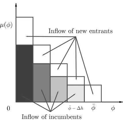
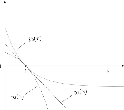
Figure 1: Productivity distribution µ(ϕ) in discrete time.
time interval ∆t, the shareµ( ¯ϕ)∆hof frontier firms moves to the left-hand neighboring segment ( ¯ϕ−∆h) because of the obsolescence of their productivities. Furthermore, the share (1−p)ϵ∆tµ( ¯ϕ−∆h)∆h of new entrants comes into segment ( ¯ϕ−∆h) during the time interval because of innovations, which attain productivity ( ¯ϕ−∆h). Therefore, the total share of firms in segment ( ¯ϕ−∆h) is larger than that in segment ¯ϕ. By maintaining these dynamics of the share of firms for each segment until exit cutoff ϕ= 0, as shown in Fig. 1, productivity distributionµ(ϕ) draws the negative slope for all ϕ.
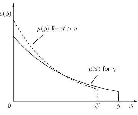
Next, we consider the economic intuition behind the Pareto exponentηof distributionµ(ϕ). According to Fig. 2, a higherηcauses a larger proportion of firms (varieties) around exit cutoffϕ= 0. According to Eq. (56), an increase in entry rateϵraises η. The reasons behind the results are as follows. New entrants tend to develop goods equipped with low productivity since productivity distributionµ(ϕ) has a negative slope because of the repeated summation of the number of new entrants and number of incumbents located in the right-hand neighboring segment. Then, promoting entry rate ϵ leads to a larger inflow of new entrants into the lower productivity region, which results in a higher η. That is, a new entrant tends to meet a low-productive incumbent and then adopt a low-productive technology because of the large number of existing low-productive firms in the economy. This mechanism causes the low-productive entrant effect after the impact of trade liberalization, as shown in Sections 4 and 5.8
There is another interpretation of η. According to Eq. (54), a higher entry rate ϵ leads to a higher exit rate, δ, in the balanced-growth equilibrium. Therefore, firms tend to locate around the exit cutoff,
ϕ= 0, as shown in Fig. 2, which implies a higher η.
8
Figure 2: Effects of Pareto exponent η on productivity distribution µ(ϕ).
4
Balanced-growth equilibrium
In this section, we show the existence of the balanced-growth equilibrium and investigate the impact of trade liberalization on the productivity distribution.
4.1 Growth rate
Consider the determination of the economic growth rate. Differentiating Eq. (12) with respect to time t, recalling that g = ˙φ∗/φ∗, noting that ˙Q/Q = ˙c/c from Eq. (10), according to Eq. (5), and simplifying
yields
˙
Q
Q =
˙
c
c =g. (59)
Therefore, the exogenous growth rate g of the world frontier technology coincides with the economic growth rate in the balanced-growth equilibrium; in other words, the model is an exogenous growth model. If we were to develop additional structures such that the growth g of the frontier technology becomes an endogenous variable, the model would become an endogenous growth model. However, this is beyond the scope of this study. Instead, Appendix C presents the model under p = 0, showing that it becomes an endogenous growth model with an exogenous productivity distribution. This result corresponds with those of Lucas and Moll (2014), Perla and Tonetti (2014), Perla et al. (2015), and Sampson (2016). Then, we show that trade liberalization raises the economic growth rate (see Proposition 5 in Appendix C).9 Further, the model under p = 0 does not have a scale effect, suggesting that the growth rate is independent of population size L(see Appendix C).
To satisfy the transversality condition (4), according to Eqs. (5) and (59), the following equation must
9
[image:17.612.198.420.66.251.2]hold:
−ρ−θc˙ c+ ˙ a a− ˙ P
P <0 ⇐⇒ r =ρ+ (θ−1)g >0. (60)
For convenience, we restate the above assumption.
Assumption 2 The equilibrium interest rate r is positive:
r=ρ+ (θ−1)g >0. (61)
4.2 Equilibrium shape of the productivity distribution
This subsection shows the existence of equilibrium value η and the balanced-growth equilibrium as well as the impact of trade liberalization on the productivity distribution.
The free-entry condition (37) determines the equilibrium Pareto exponent η of the productivity dis-tribution since the expected benefit of entryve is a function of η. To show this, defineµx as
µx ≡
∫ φ¯
φ∗
x
µ(ϕ)dϕ= e
−ηφ∗
x −p
1−p , (62)
whereµxrepresents both the share of exporting firms in a typical country and the probability of becoming an exporting new entrant conditional on drawing probability 1−p. Further, define E[·] and Ex[·] as
E[X(ϕ)] ≡∫0φ¯X(ϕ)µ(ϕ)dϕ and Ex[X(ϕ)]≡ ∫
¯
φ φ∗
x
X(ϕ)[µ(ϕ)/µx]dϕ, respectively. Then, according to Eqs. (28), (35), (36), (38), and (55), we derive the expected benefitve of entry:
ve= (1−p)vd+ (1−p)µxN vx+pvd( ¯ϕ) +pN vx( ¯ϕ), (63)
where
vd≡
∫ φ¯ 0
vd(ϕ)µ(ϕ)dϕ= [
f r+ (σ−1)g
]
E[e(σ−1)φ]−f
r +
(
f r
) [
(σ−1)g r+ (σ−1)g
]
E[e−rT(φ)] (64)
represents the expected value of the firm from a domestic market and
vx≡
∫ φ¯
φ∗
x
vx(ϕ) (
µ(ϕ)
µx ) dϕ = ( 1 τ
)σ−1[
f r+ (σ−1)g
]
Ex[e(σ−1)φ]−
( 1
τ
)σ−1
e(σ−1)φ∗x
( f r ) + ( 1 τ
)σ−1
e(σ−1)φ∗x
(
f r
) [
(σ−1)g r+ (σ−1)g
]
Ex[e−rTx(φ)],
(65)
represents the expected value of the firm from an export market conditional on exporting firms. Since (φ/φ∗)σ−1 =e(σ−1)φ,E[e(σ−1)φ] represents average relative productivity across all varieties:
E[e(σ−1)φ] =∫
¯
φ
0
e(σ−1)φµ(ϕ)dϕ=
[
η η−(σ−1)
] (
1−pe(σ−1) ¯φ
1−p
)
E[e−rT(φ)] represents the average discount factor in the event of reaching exit cutoff ϕ= 0:
E[e−rT(φ)] = ∫ φ¯
0
e−rT(φ)µ(ϕ)dϕ= (
η η+ r
g
) (
1−pe−rg
¯
φ
1−p
)
. (67)
Ex[e(σ−1)φ] represents average relative productivity conditional on exporting firms:
Ex[e(σ−1)φ] =
∫ φ¯
φ∗
x
e(σ−1)φ
(
µ(ϕ)
µx ) dϕ= ( 1 µx ) [ η η−(σ−1)
] [
e−[η−(σ−1)]φ∗
x−pe(σ−1) ¯φ
1−p
]
. (68)
Ex[e−rTx(φ)] represents the average discount factor in the event of reaching export cutoffϕ∗
x conditional
on exporting firms:
Ex[e−rTx(φ)] =
∫ φ¯
φ∗
x
e−rTx(φ)
(
µ(ϕ)
µx
)
dϕ= (
ergφ
∗
x
µx
) (
η η+gr
) [
e−(η+gr)φ
∗
x−pe− r g
¯
φ
1−p
]
. (69)
From Eq. (57),vebecomes a function ofη. Then, the free-entry condition (37) determines the equilibrium Pareto exponentη of the productivity distribution.
If we can yield an equilibrium Pareto exponentηof the productivity distribution, the other endogenous variables can automatically be determined, as shown in Section 4.3, allowing us to ensure the existence of the balanced-growth equilibrium.
Proposition 1 Suppose that Assumptions 1 and 2 hold. Then, if entry cost fe is sufficiently large, there exists a balanced-growth equilibrium.
Proof. See Appendix A.
In the equilibrium, ¯ϕ > ϕ∗
x ⇐⇒ η <(1/ϕ∗x) ln(1/p) must hold to ensure the existence of exporting
firms. A sufficiently largefe causes a sufficiently small equilibriumη, which ensures that ¯ϕ > ϕ∗
x. More
precisely, the large fixed cost feof entry discourages the entry of new firms, which raises average relative
productivity because new entrants tend to draw a lower existing productivity from distribution µ(ϕ). Therefore, the discouragement of new entry caused by a large fe raises average relative productivity, which implies a lower η, as shown in Fig. 2. Then, in Proposition 1, we require the condition that fe is
sufficiently large to ensure the existence of the balanced-growth equilibrium with ¯ϕ > ϕ∗
x. However, when p→0, ¯ϕ > ϕ∗
x ⇐⇒ η <(1/ϕ∗x) ln(1/p) is satisfied without the assumption of a sufficiently large fe. See
Appendix B for more details, where Lemma 3 shows the uniqueness ofη under the additional assumption
p→0.
Proposition 2 Suppose that Assumptions 1 and 2 as well as p→0 hold. Then,
(ii) A decrease in the fixed cost fx of the exporting varieties increases the equilibrium Pareto exponent η of the productivity distribution.
Proof. See Appendix B.
Proposition 2 implies that trade liberalization via a reduction in τ has a negative effect on average productivity in the economy, as implied in Fig. 2. The following average productivities E[e(σ−1)φ] and
Ex[e(σ−1)φ] affect welfare, as shown in Section 4.3. Therefore, we now conduct the comparative statics of
these average productivities.
Proposition 3 Suppose that Assumptions 1 and 2 as well as p→0 hold. Then,
(i) A decrease in iceberg cost τ decreases average relative productivityE[e(σ−1)φ] across all varieties;
(ii) A decrease in iceberg cost τ decreases average relative productivity Ex[e(σ−1)φ] across all exporting
(imported) varieties;
(iii) A decrease in the fixed cost fx of the exporting varieties decreases average relative productivity
E[e(σ−1)φ] across all varieties;
(iv) A decrease in the fixed cost fx of the exporting varieties decreases average relative productivity
Ex[e(σ−1)φ]across all exporting (imported) varieties.
Proof. See Appendix B.
Trade liberalization via a reduction in τ or fx increases the equilibrium Pareto exponent η of the productivity distribution. This then reduces E[e(σ−1)φ] and E
x[e(σ−1)φ] for the following reason. A
reduction in τ orfx increases the expected entry value ve for a given η since each new entrant expects to earn larger export profits because of lower trade barriers. This then fosters the entry of firms into the market. New entrants tend to have low productivity since productivity distributionµ(ϕ) has a negative slope, as explained in Section 3.2. Therefore, fostering the entry of new firms through trade liberalization reducesE[e(σ−1)φ] andEx[e(σ−1)φ] because of the diffusion of inferior existing technologies. That is, trade
liberalization causes the low-productive entrant effect.
4.3 Welfare measure
To prepare for the numerical welfare analysis in Section 5, we consider the determination of welfare and the other variables in the model.
The initial consumption level or real income is the steady-state welfare measure in the model. Define
asset value is aL=M v=M(vd+N µxvx), according to Eqs. (6) and (42), equilibrium consumption per
capita is
c= 1 +ra
P , (70)
where asset value per capita is
a= M v
L =
M(vd+N µxvx)
L . (71)
That is, initial consumption is equal to real income. As we develop the exogenous growth model, we see that initial consumption c, determined from Eq. (70), only affects welfare in the balanced-growth equilibrium. Therefore, the variable cis the welfare measure in the presented model.
Derive the price index as follows:
P = (M p1d−σ +N Mxp1x−σ)
1
1−σ, (72)
where
p1d−σ ≡
∫ φ¯ 0
pd(ϕ)1−σµ(ϕ)dϕ=
(
σ σ−1
)1−σ
E[e(σ−1)φ](φ∗)σ−1 (73)
p1x−σ ≡
∫ φ¯
φ∗
x
px(ϕ)1−σ (
µ(ϕ)
µx
)
dϕ= (
σ σ−1
)1−σ
τ1−σEx[e(σ−1)φ](φ∗)σ−1. (74)
The variables pd and px represent the weighted averages of domestic prices across all domestic varieties
and of import prices across all imported varieties, respectively. Both pd and px are functions ofη. Note that E[e(σ−1)φ](φ∗)σ−1 represents average absolute productivity φσ−1 sinceφσ−1 = (φ/φ∗)σ−1(φ∗)σ−1 =
e(σ−1)φ(φ∗)σ−1. Then, noting Eq. (57) and ¯ϕ= ln( ¯φ/φ∗), the average value ofφσ−1isE[e(σ−1)φ](φ∗)σ−1=
E[e(σ−1)φ]e−(σ−1) ¯φ( ¯φ)σ−1 for a given exogenous state ¯φ. Similarly,E
x[e(σ−1)φ] represents average absolute
productivityφσ−1conditional on imported varieties, as given byE
x[e(σ−1)φ](φ∗)σ−1 =Ex[e(σ−1)φ]e−(σ−1) ¯φ( ¯φ)σ−1
for a given exogenous state ¯φ.
Next, consider the labor market equilibrium, which determines the number M of domestic varieties and the number Mx of exporting varieties. Derive average labor demand for production as follows:
l≡
∫ φ¯ 0
l(ϕ)µ(ϕ)dϕ=ld+µxN lx, (75)
where
ld≡
∫ φ¯ 0
ld(ϕ)µ(ϕ)dϕ=f(σ−1)E[e(σ−1)φ] +f (76)
represents average labor demand for a domestic market and
lx ≡
∫ φ¯
φ∗
x
lx(ϕ) (
µ(ϕ)
µx ) dϕ= ( 1 τ
)σ−1
f[(σ−1)Ex[e(σ−1)φ] +e(σ−1)φ
∗
x]. (77)
market-clearing condition (40), the number of domestic varieties is
M = L
l+ϵfe
. (78)
Notingϵ=gη/(1−p) from Eq. (56), the right-hand side of Eq. (78) becomes a function ofη. Then, if we yield an equilibriumη, Eq. (78) determines the equilibrium numberM of domestic varieties. Mx=µxM
determines the number Mx of exporting varieties in a typical country.
Following Arkolakis et al. (2012), Perla et al. (2015), and Sampson (2016), we can rewrite initial consumptioncby using the domestic trade share. Defineλas the domestic trade share (i.e., the proportion of domestic revenues in total revenues):
λ≡ M
∫φ¯
0 Rd(ϕ)µ(ϕ)dϕ
M∫0φ¯R(ϕ)µ(ϕ)dϕ , (79)
where
R(ϕ)≡Rd(ϕ) +N Rx(ϕ) (80)
represents the total revenue of a firm whose productivity isϕ.
Rd(ϕ)≡pd(ϕ)qd(ϕ) =σe(σ−1)φf (81)
represents the domestic revenue of a firm whose productivity is ϕ and qd(ϕ) is the amount of the
inter-mediate good under domestic price pd(ϕ).
Rx(ϕ)≡px(ϕ)qx(ϕ) =σ
( 1
τ
)σ−1
e(σ−1)φf (82)
represents the exporting revenue of a firm whose productivity is ϕ and qx(ϕ) is the amount of the
inter-mediate good under exporting price px(ϕ). Then, Eq. (79) becomes
λ= E[e
(σ−1)φ]
E[e(σ−1)φ] +N(1
τ
)σ−1
µxEx[e(σ−1)φ]
. (83)
By using the domestic trade share (83), the price index (72) becomes
P =
(
σ σ−1
)
λ
1
σ−1
M
1
σ−1 {E[e(σ−1)φ]} 1
σ−1
φ∗
. (84)
Therefore, initial consumption is
c= (
σ−1
σ
) ( 1
λ
) 1
σ−1
Aggregate absolute productivity
z }| {
M
1
σ−1
{
E[e(σ−1)φ]}
1
σ−1
φ∗
| {z }
Average absolute productivity
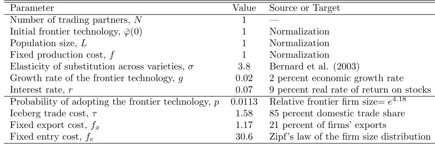
Table 1: Calibration
Parameter Value Source or Target Number of trading partners, N 1 —
Initial frontier technology, ¯φ(0) 1 Normalization Population size,L 1 Normalization Fixed production cost,f 1 Normalization Elasticity of substitution across varieties,σ 3.8 Bernard et al. (2003)
Growth rate of the frontier technology,g 0.02 2 percent economic growth rate Interest rate,r 0.07 9 percent real rate of return on stocks Probability of adopting the frontier technology,p 0.0113 Relative frontier firm size=e4.18 Iceberg trade cost, τ 1.58 85 percent domestic trade share Fixed export cost,fx 1.17 21 percent of firms’ exports
Fixed entry cost,fe 30.6 Zipf’s law of the firm size distribution
Then, the following three variables determine initial consumption and welfare: domestic trade share λ, aggregate absolute productivityMσ−11 {E[e(σ−1)φ]}
1
σ−1
φ∗, and per capita asset levela.
5
Numerical analysis
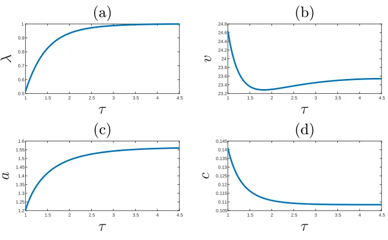
In this section, we numerically show the effect of trade liberalization via a reduction inτ on average and aggregate productivities and welfare in the balanced-growth equilibrium. Since the effect of a reduction infx is similar to that in τ, we report the case offx in Appendix D.
5.1 Calibration
To quantify the productivity and welfare gains or losses from trade liberalization, we calibrate the model. The top panel of Table 1 reports the normalizations and preselected parameters. We set the number of trading partners N to 1.10 That is, we investigate the counterfactual impact of the bilateral trade agreements between symmetric countries. The initial frontier technology ¯φ(0) is an initial state variable, which only affects the scale of absolute exit cutoffφ∗. We normalize this to set ¯φ(0) = 1. According to Eq.
(78), population sizeL only proportionally affects the number M of domestic varieties since entry rateϵ
and aggregate labor demandlare independent ofL. That is,Ldetermines the scale ofM. We normalize this to set L= 1. The parameter choice of fixed production costf has no substantive effect on η, which is a key variable in this paper. Indeed, according to Eq. (17), relative exporting cost τσ−1fx/f affects
export cutoffϕ∗
x. Thus, from Eq. (37), the relative exporting cost and relative fixed entry costfe/f affect
the Pareto exponent η of the productivity distribution. Therefore, we normalize fixed production cost
f to unity. The elasticity of substitution across varieties of 3.8 comes from Bernard et al. (2003). This value implies that the gross markup (the ratio of price to marginal cost) is σ/(σ−1) = 1.36, which is in the range of 1.05–1.4 estimated by Norrbin (1993) and Basu (1996).11 The growth rate g of the frontier
10
GivenN = 5, recalibrating the model to match the data in Table 1 yieldsp= 0.0113,τ= 2.80,fx= 0.23, andfe= 30.5.
Further, givenN = 10, recalibrating yieldsp= 0.0113, τ = 3.59,fx = 0.12, andfe = 30.6. Under both sets of calibrated
parameters withN= 5 andN = 10, we confirm that the results described in Sections 5.2 and 5.3 are generally unchanged.
11
The markup σ/(σ−1) ∈ [1.05,1.4] implies that σ ∈ [3.5,21]. Then, given σ = 3.5, recalibrating yields p = 0.0109,
1 1.5 2 2.5 3 3.5 4 4.5 2.8
[image:24.612.218.392.75.217.2]2.9 3 3.1 3.2 3.3 3.4 3.5
Figure 3: The impact of iceberg trade cost τ on the Pareto exponent η of the productivity distribution.
technology is set to 0.02 to target a 2 percent per capita GDP growth rate in the United States since World War II. The inverse of the intertemporal elasticity of substitutionθ and discount rateρ affect the model only through interest rate r. Then, it is sufficient to specify the value of r. Mehra and Prescott (2003) report a 9 percent average real rate of return on stocks in the United States since World War II. In the model, the real rate of return isr−P /P˙ =r+g. Giveng = 0.02, we set r = 0.07 to match the historical real rate of return on stocks.12
Given the normalizations and preselected parameters, the bottom panel of Table 1 reports the pa-rameters set to target the moments in the data. Benhabib et al. (2017) report that the mean of the ratio of the 90th to 10th percentiles of employment across industries for 1980–2014 in the United States is
e4.18. The 90th percentile of employment is a proxy for the frontier employment and the 10th percentile
is a proxy for the least productive firm’s employment. We set p = 0.0113 to match l( ¯ϕ)/l(0) = e4.18.
Benhabib et al. (2017) also report that the mean of the ratio of the 90th to 10th percentiles of revenue is
e4.39. Under the calibrated parameters in Table 1, our model provides R( ¯ϕ)/R(0) =e4.48, which is close
to the data. Ramondo et al. (2016) report that the average U.S. domestic trade share in manufacturing over 1996–2001 is 85 percent. To match λ= 0.85, we set τ = 1.58. We choose fx = 1.17 to match the proportion of U.S. manufacturing plants that exported in 1992, µx= 0.21, as reported by Bernard et al. (2003). Luttmer (2007) estimates η/(σ−1) = 1.06 based on the distributions of firm size (employment). To satisfyη/(σ−1) = 1.06, we set fe= 30.6.13
5.2 Productivity gains from trade liberalization
Given the calibrated parameters in Table 1, we study the impact of trade liberalization via a reduction inτ on the productivity measures. As shown in Fig. 3, the reduction in τ increases the Pareto exponent
data in Table 1. We confirm that σ= 9.65 is the maximum value that has a solution for the calibration. Givenσ= 9.65, recalibrating yieldsp= 0.0139, τ = 1.16,fx= 1.18, andfe= 13.8. Under both sets of calibrated parameters withσ= 3.5
andσ= 9.65, we confirm that the results described in Sections 5.2 and 5.3 are generally unchanged.
12
Previous studies may set a lower interest rate,r. Then, givenr= 0.01, 0.02, 0.03, 0.04, 0.05, and 0.06, we recalibrate the model to match the data in Table 1. Under each set of calibrated parameters, we confirm that the results described in Sections 5.2 and 5.3 are generally unchanged.
13
1 1.5 2 2.5 3 3.5 4 4.5 3
3.5 4 4.5
1 1.5 2 2.5 3 3.5 4 4.5 0.05
0.055 0.06 0.065 0.07 0.075 0.08 0.085
1 1.5 2 2.5 3 3.5 4 4.5 0.045
0.05 0.055 0.06 0.065 0.07
1 1.5 2 2.5 3 3.5 4 4.5 3.5
3.6 3.7 3.8 3.9 4 4.1
[image:25.612.114.495.77.307.2]10-3
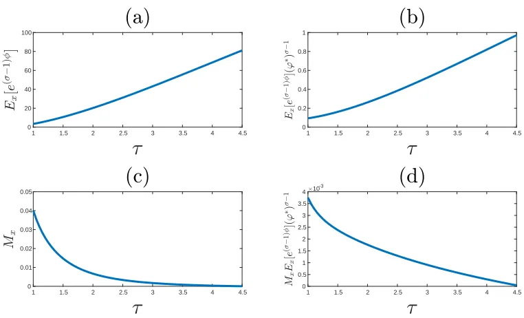
Figure 4: The impact of iceberg trade costτ on the productivities and the mass of domestic varieties. The vertical axis in Fig. (a) represents average productivity relative to the exit cutoff. The vertical axis in Fig. (b) represents average productivity. The vertical axis in Fig. (c) represents the number of domestic varieties. The vertical axis in Fig. (d) represents aggregate productivity.
η of the productivity distribution. This numerical result is consistent with Proposition 2, which is the analytical result under p→0. The increase in η implies the low-productive entrant effect, which reduces average relative productivity E[e(σ−1)φ], as shown in Fig. 4(a). That is, trade liberalization induces
low-productive firms to enter the market, which reduces average relative productivity. The numerical result is also consistent with result (i) of Proposition 3 and result (i) of Lemma 2 in Appendix A. As in the Melitz (2003) model, trade liberalization also has the resource reallocation effect caused by market selection. That is, the reduction in τ increases exit cutoff productivity φ∗. This is because trade liberalization reduces
price index P, as explained in Section 5.3, which reduces demand for each variety (8) and negatively affects the domestic profit (11). That is, trade liberalization fosters competition between varieties. Thus, according to Eq. (12), trade liberalization has a positive effect on exit cutoffφ∗through price indexP. In
addition, trade liberalization has a negative effect on exit cutoff φ∗ because of the increase in aggregate
demand Q = cL for the goods (see Fig. 6(d)). However, the negative effect on φ∗ is sufficiently small
to ensure that trade liberalization increases exit cutoff φ∗. Consequently, trade liberalization facilitates
the exit of low-productive firms, and thus the (labor) resources employed by the exiting low-productive firms can be reallocated toward high-productive firms. This resource reallocation effect contributes to an increase in average absolute productivity in the economy. As shown in Fig. 4(b), the resource reallocation effect dominates the low-productive entrant effect; that is, the reduction in τ increases average absolute productivity E[e(σ−1)φ] (φ∗)σ−1. This numerical result is consistent with analytical result (ii) of Lemma
1 1.5 2 2.5 3 3.5 4 4.5 0
20 40 60 80 100
1 1.5 2 2.5 3 3.5 4 4.5 0
0.2 0.4 0.6 0.8 1
1 1.5 2 2.5 3 3.5 4 4.5 0
0.01 0.02 0.03 0.04 0.05
1 1.5 2 2.5 3 3.5 4 4.5 0
0.5 1 1.5 2 2.5 3 3.5
[image:26.612.114.495.76.307.2]4 10-3
Figure 5: The impact of iceberg trade cost τ on productivities conditional on exporting firms and the mass of exporting varieties. The vertical axis in Fig. (a) represents average productivity relative to the exit cutoff conditional on exporting firms. The vertical axis in Fig. (b) represents average productivity conditional on exporting firms. The vertical axis in Fig. (c) represents the number of exporting varieties. The vertical axis in Fig. (d) represents aggregate productivity conditional on exporting firms.
As in the Melitz (2003) model, according to Fig. 4(c), trade liberalization reduces domestically produced varietiesM, which has a negative effect on aggregate absolute productivity in the economy. Fig. 4(d) shows the non-monotonic (U-shaped) effect of trade liberalization on aggregate absolute productivity
ME[e(σ−1)φ] (φ∗)σ−1. This result implies that the sum of the negative effect on M and low-productive
entrant effect may dominate the resource reallocation effect, and thus trade liberalization may reduce aggregate productivity. Melitz (2003) shows that the resource reallocation effect dominates the negative effect on M, and thus trade liberalization always increases aggregate productivity. On the contrary, by adding the low-productive entrant effect into the Melitz (2003) model, we yield the non-monotonic (U-shaped) relationship between trade liberalization and aggregate productivity.14 Then, according to Eq. (85), trade liberalization has a non-monotonic effect on initial consumption and welfare via aggregate productivity.
Next, we examine the impact of a reduction in τ on productivities conditional on the exporting (imported) varieties. As shown in Fig. 5(a), trade liberalization via the reduction in τ reduces average relative productivity conditional on the exporting varieties Ex[e(σ−1)φ], which is a result of the
low-productive entrant effect. This numerical result is consistent with result (ii) in Proposition 3. Fig.
14
5(b) shows that trade liberalization reduces average absolute productivityEx[e(σ−1)φ] (φ∗)σ−1 conditional
on exporting firms. This finding implies that the low-productive entrant effect dominates the resource reallocation effect when we focus on the average productivity of exporting firms.
According to Fig. 5(c), trade liberalization increases exporting varieties Mx = µxM, which has a
positive effect on aggregate absolute productivity conditional on exporting firms. Figs. 4(c) and 5(c) imply that trade liberalization increases the shareµxof exporting varieties. Trade liberalization has both positive and negative effects on shareµx. According to Eqs. (17) and (62), the reduction inτ has a positive
effect on shareµx because of the reduction in trade barriers. On the contrary, the reduction inτ increases
η, which results in the low-productive entrant effect. That is, trade liberalization increases the share of low-productive firms, which reduces the share µx of high-productive exporting firms. Consequently, we
have a dominant positive effect onµx, and thus the reduction inτ increasesµx. Further, the increase in
µx is sufficiently strong to raise Mx. Then, Fig. 5(d) shows that the reduction in τ increases aggregate absolute productivityMxEx[e(σ−1)φ] (φ∗)σ−1 conditional on exporting firms. This is because the positive
effect on Mx and resource reallocation effect dominate the low-productive entrant effect.
We now consider the reason behind the negative effect of trade liberalization on M, as shown in Fig. 4(c). The labor market-clearing condition (78) determines the number of domestic varietiesM. According to Eqs. (76) and (77), and Figs. 4(a) and 5(a), the reduction inτ causes the low-productive entrant effect, which has a negative effect on average labor demand ldfor a domestic market and average labor demand
lx for an export market conditional on exporting firms. However, the reduction in τ also has a positive effect onlx because it contributes to an increase in the exporting profit (16) and thus raises the average labor demand lx of exporting firms. Furthermore, the reduction in τ raises the share µx of exporting firms, according to Eq. (75), which contributes to an increase in average labor demand l. In addition, according to Fig. 3 andϵ=gη/(1−p), the reduction inτ increases entry rateϵbecause of the reduction in trade barriers. Consequently, trade liberalization must reduce the domestic varietiesM to ensure the labor market-clearing condition because it has dominant positive effects on average labor demandlacross all firms and labor demand ϵfe for entering firms.
5.3 Welfare gains from trade liberalization
Given the calibrated parameters in Table 1, we study the impact of trade liberalization via a reduction inτ
on welfare. Fig. 6(d) implies that the reduction inτ increases welfare in the balanced-growth equilibrium. We consider the reason behind this result.
Fig. 6(a) reports that the reduction in τ decreases domestic trade share λ. According to Eq. (83) and Fig. 5(a), trade liberalization has a positive effect onλ because of the reduction in average relative productivity Ex[e(σ−1)φ] conditional on exporting firms. However, Fig. 6(a) implies that this positive
effect is relatively small. The following three dominant effects contribute to the reduction in domestic trade share λ as τ decreases: an increase in the share µx of exporting firms, the reduction in relative productivityE[e(σ−1)φ] due to the low-productive entrant effect, and an increase in the exporting revenue for each firm because of the reduction in marginal costs. As shown in Eqs. (84) and (85), the reduction in domestic trade shareλhas a positive effect on initial consumptionc and welfare via price indexP.
1 1.5 2 2.5 3 3.5 4 4.5 0.5
0.6 0.7 0.8 0.9 1
1 1.5 2 2.5 3 3.5 4 4.5 23.2
23.4 23.6 23.8 24 24.2 24.4 24.6 24.8
1 1.5 2 2.5 3 3.5 4 4.5 1.2
1.25 1.3 1.35 1.4 1.45 1.5 1.55 1.6
1 1.5 2 2.5 3 3.5 4 4.5 0.105
[image:28.612.113.496.76.313.2]0.11 0.115 0.12 0.125 0.13 0.135 0.14 0.145
Figure 6: The impact of iceberg trade costτ on domestic trade share λ, average assets across all firmsv, per capita assetsa, and initial consumption c.
v. This is because trade liberalization has the following positive or negative effects on v. The low-productive entrant effect reducesvby increasing the share of low-productive firms. On the contrary, trade liberalization increases the shareµx of exporting firms, and thus it raises v. Further, the reduction in τ
increases exporting profits because of the reduction in marginal costs, which increases v. Consequently, as shown in Fig. 6(b), trade liberalization has a non-monotonic effect on the average value of the firm,
v. On the contrary, as shown in Fig. 6(c), the reduction in τ monotonically reduces per capita assets
a. Noting that a = M v/L, the additional negative effect of M on a contributes to the reduction in a. Then, the reduction inahas a negative effect on initial consumption and welfare because it reduces asset income.
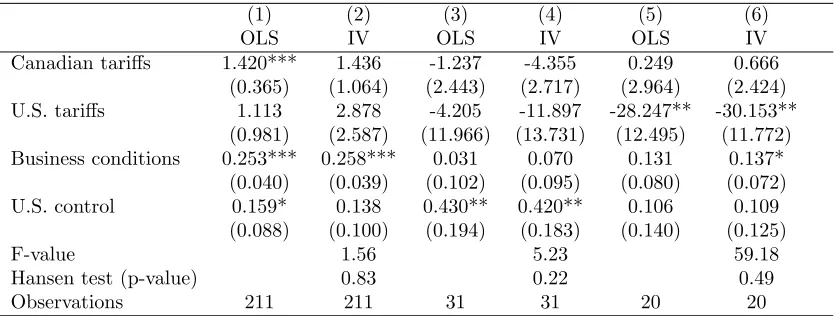
Table 2: Effects of trade liberalization on labor productivity
(1) (2) (3) (4) (5) (6)
OLS IV OLS IV OLS IV
Canadian tariffs 1.420*** 1.436 -1.237 -4.355 0.249 0.666 (0.365) (1.064) (2.443) (2.717) (2.964) (2.424) U.S. tariffs 1.113 2.878 -4.205 -11.897 -28.247** -30.153**
(0.981) (2.587) (11.966) (13.731) (12.495) (11.772) Business conditions 0.253*** 0.258*** 0.031 0.070 0.131 0.137*
(0.040) (0.039) (0.102) (0.095) (0.080) (0.072) U.S. control 0.159* 0.138 0.430** 0.420** 0.106 0.109
(0.088) (0.100) (0.194) (0.183) (0.140) (0.125)
F-value 1.56 5.23 59.18
Hansen test (p-value) 0.83 0.22 0.49
Observations 211 211 31 31 20 20
Notes: The dependent variable is labor productivity. All the estimations include a constant term, although we do not report the results here. The asterisks ***, **, and * indicate the 1%, 5%, and 10% significance levels, respectively. The numbers in parentheses are heteroskedasticity-robust standard errors.
6
Empirical evidence
Fig. 4(d) shows the non-monotonic relationship between trade liberalization and productivity. In this section, we revisit Trefler’s (2004) study of the effect of the Canada-U.S. FTA on the Canadian manufac-turing sector and confirm the negative impact of trade liberalization in certain circumstances. By using his dataset of four-digit standard industrial classification data (213 industries) in Canada, we estimate the baseline specification:
(∆yi1−∆yi0) =θ+βCA(∆τiCA1 −∆τiCA0 )+βU S(∆τiU S1 −∆τiU S0 )+δ(∆bi1−∆bi0)+γ(∆yiU S1 −∆yU Si1 )+vi. (86)
Following the notation presented by Trefler (2004), we let yit be labor productivity in industry i in period t. ∆yi1 is the average annual log change in labor productivity in the FTA period, specifically
∆yi1 = (lnyi,1996−lnyi,1998)/(1996−1988). Likewise, ∆yi0 is the same in the pre-FTA period, specifically
∆yi0 = (lnyi,1986−lnyi,1980)/(1986−1980). ∆τik1 is the change in the FTA-mandated tariff concessions
extended by Canada (the United States) to the United States (Canada) when k indexes CA (US). ∆τk i0
is the average change in tariff concessions when industry i is the automotive sector and zero otherwise. ∆bi captures the business conditions and is the proportion of labor productivity driven by movements in GDP and the real exchange rate. ∆yU S
i is labor productivity in the United States. vi is an error term.
See Trefler (2004) for additional details.
Table 2 shows the estimation results for labor productivity. While Trefler (2004) rescales βCA and
βU S to pay attention to the most impacted, import-competing group of industries, we multiply these
[image:29.612.98.516.104.262.2]