An environmental audio based context recognition system using smartphones

(1)

University of Twente

Master Thesis

An Environmental Audio–Based Context

Recognition System Using Smartphones

Author:

Gebremedhin T. Abreha

Supervisor:

Dr. Nirvana Meratnia Committee:

Prof. Paul Havinga

Ir. Bert Molenkamp

A thesis submitted in fulfilment of the requirements

for the degree of Master of Science in Embedded Systems

Pervasive Systems Chair

Faculty of Electrical Engineering, Mathematics and Computer Science

(2)

University of Twente

Faculty of Electrical Engineering, Mathematics and Computer Science

Master of Science in Embedded Systems

An Environmental Audio–Based Context Recognition System Using

Smartphones

by Gebremedhin T. Abreha

Abstract

Environmental sound/audio is a rich source of information that can be used to infer

a person’s context in daily life. Almost every activity produces some sound patterns,

e.g., speaking, walking, washing, or typing on computer. Most locations have usually

a specific sound pattern too, e.g., restaurants, offices or streets. This thesis addresses

the design and development of an application for real-time detection and recognition

of user activities using audio signals on mobile phones. The audio recognition

applica-tion increases the capability, intelligence and feature of the mobile phones and, thus,

increases the convenience of the users. For example, a smartphone can automatically

go into a silent mode while entering a meeting or provide information customized to

the location of the user. However, mobile phones have limited power and capabilities

in terms of CPU, memory and energy supply. As a result, it is important that the

de-sign of audio recognition application meets the limited resources of the mobile phones.

In this thesis we compare performance of different audio classifiers (k-NN, SVM and

GMM) and audio feature extraction techniques based on their recognition accuracy and

computational speed in order to select the optimal ones. We evaluate the performance

of the audio event recognition techniques on a set of 6 daily life sound classes (coffee

machine brewing, water tape (hand washing), walking, elevator, door opening/closing,

and silence ). Test results show that the k-NN classifier (when used with mel-frequency

cepstral coefficients (MFCCs), spectral entropy (SE) and spectral centroid (SC) audio

features) outperforms other audio classifiers in terms of recognition accuracy and

execu-tion time. The audio features are selected based on simulaexecu-tion results and proved to be

(3)

iii

an Android app (on mobile phones) using the k-NN classifier and the selected optimal

audio features. The application continuously classifies audio events (user activities) by

analyzing environmental sounds sampled from smartphone’s microphone. It provides a

user with real-time display of the recognized context (activity). The impact of other

parameters such as analysis window and overlapping size on the performance of audio

recognition is also analyzed. The test result shows that varying the parameters does not

have significant impact on the performance of the audio recognition technique.

More-over, we also compared online audio recognition results of the same classifier set (i.e.,

(4)

Acknowledgements

First of all, I would like to thank Almighty God, who has blessed and guided me so that

I am able to accomplish this thesis.

In this very special occasion, I would like to express my deepest gratitude and

appreci-ation to my Supervisor, Dr. Nirvana Meratnia, who gave her valuable time, guidance,

advice, criticism and corrections to the thesis from the beginning till the end. She was

always available for my questions and she was positive and gave generously her time

and vast knowledge. I also want to thank all of the lecturers and professors of the

Fac-ulty who have thought and guided me during the years of my study at the University.

In addition, I would like to thank the University of Twente Scholarship for providing

me with financial help and funding, without which it would not have been possible to

successfully finish my study.

(5)

List of Figures

1.1 Project Overview Components . . . 7

2.1 Rectangular Window . . . 15

2.2 Hamming Window . . . 15

3.1 MFCC Process . . . 27

4.1 k-NN Classification . . . 33

4.2 Gaussian Mixture Models . . . 35

4.3 SVM Classification . . . 36

4.4 SVM Mapping . . . 37

5.1 Pre-Processing and Feature Extraction . . . 40

5.2 Signal before Pre-Emphasis . . . 42

5.3 Signal after Pre-Emphasis . . . 42

5.4 Framing Process . . . 43

5.5 Windowing Process with Hamming Window . . . 43

5.6 Classifier Implementation . . . 47

5.7 Post-process Class label Merging Class Sequences . . . 49

6.1 k-NN Performance vs k . . . 59

6.2 SVM Performance for Different Kernel Functions . . . 62

6.3 Low GMM Performance for Small Datasets . . . 66

6.4 GMM Performance for Different Number of GMM Components, k . . . . 67

6.5 Individual Feature Performance . . . 72

7.1 The Classification Process of On-line Audio Recognition . . . 75

7.2 GUI of Android App . . . 76

7.3 On-line phase, Execution Time . . . 79

7.4 Continuous Sound Event Recognition . . . 81

7.5 On-line:- Heap Memory Usage. . . 83

7.6 On-line:- Overall Memory Usage . . . 84

(8)

(9)

List of Tables

6.1 Small Dataset . . . 55

6.2 Big Dataset . . . 55

6.3 k-NN: Confusion Matrix for Small Dataset. . . 60

6.4 k-NN: Confusion Matrix for Big Dataset . . . 60

6.5 SVM performance Confusion Matrix (for Small Dataset) . . . 63

6.6 SVM performance Confusion Matrix (for Big Dataset) . . . 63

6.7 Low GMM Performance Confusion Matrix (LOO) . . . 66

6.8 GMM-Confusion Matrix for Big Dataset . . . 67

6.9 Summary of Classifiers’ Comparison . . . 69

6.10 Parameter Selection . . . 70

(10)

(11)

Dedicated to my Parents.

(12)

(13)

Chapter 1

Introduction

As modern science and information technology advances, device sizes are becoming

smaller and more operations are now feasible on smaller devices. For instance, mobile

devices, such as smart-phone, not only do they work as a telephone, but also their role

now have expanded to taking pictures, texting/receiving messages, playing music/videos,

keeping appointments, etc. Nevertheless, people still want to access or obtain more

intelligent and intuitive knowledge anytime and anywhere using their mobile devices.

The rapid increase in speed and capacity of smart mobiles or embedded devices equipped

with sensors and powerful processors (CPUs) is expected to allow the inclusion of more

applications that can increase the capability, intelligence and feature of mobile devices.

One of the key anticipated future capabilities of smart devices is Context Awareness

(CA). CA enables mobile devices to sense and recognize user’s contextual information

such as user activities, surrounding environment, and provide context relevant

informa-tion for user’s current needs. Many sources such as microphone, camera, gyroscope,

accelerometer, luminance, Global Positioning System (GPS), and etc., are available for

sensing and capturing various types of contextual information. In audio based context

awareness systems, environmental sounds are used to obtain contextual information such

as the type of environment (location context), activities (what a user is doing) and what

activities/evets are going on in a specific location [1–6].

Audio based CA applications provide mobile device (phone) with the ability to

auto-matically know the context of a given environment and use its knowledge to respond to

the mobile user in the most appropraite way. In other words, the CA system enables

(14)

Chapter 1. Introduction 2

a cellphone to change automatically the notification or operation mode based on the

knowledge of the user’s surrounding. For example, a mobile phone can dynamically

switch from a ringing mode to a vibration or silence mode when a user enters into a

meeting room or holds a presentation, and in contrast, it may ring louder when the user

is in a noisy place, e.g. a street. Similarly, if a user receives a call while she or he is

in a meeting, the mobile phone can automatically send a message to the caller saying

that she or he is in a meeting. Audio based CA systems has been also used in robot

navigation [7,8], audio based surveillance systems [9], audio based forensics [10], hearing

aid [11], home-monitoring environment for assisting elderly people living alone in their

own home [12,13] or for a smart home [14].

Auditory signals are chosen for a number of reasons. Firstly, among the human senses,

hearing is second only to vision in recognizing social and conceptual settings; this is

due partly to the richness in information of audio signals. Secondly, cheap but practical

microphones can be embedded in almost all types of places or mobile devices, including

PDAs and mobile phones. Thirdly, auditory-based context recognition consumes

signif-icantly fewer computing resources than camera-based context recognition. In addition,

unlike visual sources of information such as camera and video, audio information cannot

be obscured by solid objects and it is multidirectional, i.e., it can be received from any

direction. Additionally, audio data is less sensitive to the location and orientation of the

phone as compared with other common sensors such as cameras and accelerometers.

Humans can easily segregate and recognize one sound source from an acoustic mixture,

such as certain voice from a busy (noisy) background including other people talking

and music. The study of sound analysis, which aims to separate and recognize mixture

of sound sources present in an auditory scene, is broadly known in the literature as

Computational Auditory Scene Analysis (CASA) [15]. CASA aims to enable computers

hear and understand audio content much as humans do. Due to its broad nature, the

study of CASA is usually dealt with by dividing into three main research topic areas [15]:

1) Context awareness (recognition of audio context) - dealing with recognition of context

such as location or activity happening in a given environment. (answers “where” e.g.

restaurant, inside a car) based on the audio information/events, 2) Sound event detection

and recognition – dealing with categorization of individual sound events present in the

(15)

audio classification – dealing with classification and recognition of the contents of audio

signals, e.g., for audio content retrieval, indexing, and audio based searching.

This thesis deals with sound event detection and recognition also referred as

environ-mental sound/audio recognition (ESR). The detected sound events can then be used for

the purpose of context recognition. For example, the sound event of keyboard typing

helps to know that the user is in his/her office, which is, in this case, location context.

1.1 General Challenges of Environmental Audio

Classifi-cation and Recognition

In this section, main challenges that are faced in ESR and classification are pointed out.

Unlike speech or music signals, environmental acoustic signals are difficult to model

due to its high unpredictable nature. Speech or music can be categorized to structured

sounds due to their formantic or harmonic structure characteristic whereas

environmen-tal sounds, on the other side, are typically unstructured, which have a broad noise-like

flat spectrum and diverse variety of signal composition and are difficult to build models.

Analysis of real-world audio that consists of a rich mix of naturally occurring sounds

such as the environmental sound is complex. As a result, classification and processing

of environmental sound is generally more cumbersome compared with that of speech or

music. The following are the general challenges that are faced during the design and

implementation of ESR technique:

• Overlap in time and/or frequency content- Different sound events can hap-pen at the same time which makes recognition of the type of sound event difficult.

This leads to two challenging tasks: detection of individual sound events within

the audio scene (segmentation) and classification. A system involved in the first

task has as a goal to cluster mixed sound events from different sources into their

corresponding source type, or try to segment the audio into pieces that represent

a single occurrence of a specific event class by estimating the start and end time of

each event and if necessary separating it from other overlapping events. The aim of

the second task is to characterize and identify the type of sound event (e.g., label

(16)

events that constitute a natural auditory scene (environmental sound) create an

acoustic mixture signal that is more difficult to handle.

• Dynamic nature of environment – Apart from containing a wide variety of sound classes, environmental sound has a dynamic nature, i.e., new sound types

(classes) can appear and existing sound classes can disappear randomly at any

time. Similarly, mobile devices can move from one environment to another

envi-ronment and may encounter new types of sound. Therefore, the ESR technique

has to deal with and adapt to the dynamic nature of an environmental sound.

• Selection of feature set- Audio features have a significant impact on the recog-nition accuracy. Thus, the defirecog-nition and extraction of the right type of feature sets

is a very important step in ESR. However, it is challenging step too. What feature

types we define and how we use them depends on the type of application. For

example, audio features used for audio classification in indoors might not perform

well when used for the classification of types of sounds in outdoor areas.

1.2 Smartphone Specific Challenges

In addition to the above mentioned general challenges, there are also special challenges

that have to be dealt with in order to implement audio based CA technique on

mo-bile devices/smartphones. While smartphones continue to provide more computation,

memory, storage, sensing, and communication bandwidth, the phone is still a

resource-limited device if complex signal processing and inference are required. Signal processing

and machine learning algorithms can stress the resources of the phones in different ways:

some require the CPU to process large volumes of sensor data (e.g., interpreting audio

data), some need frequent sampling of energy expensive sensors (e.g., GPS), while

oth-ers require real-time inference. Different applications place different requirements on the

execution of these algorithms. For example, for applications that are user initiated the

latency of the operation is important. Applications (e.g., healthcare) that require

con-tinuous sensing will often require real-time processing and classification of the incoming

stream of sensor data. We believe continuous sensing can enable a new class of real-time

(17)

Early deployments of phone sensing systems tended to trade off accuracy for lower

resource usage by implementing algorithms that require less computation or a reduced

amount of sensor data. Limited power supply and real time requirement are the most

common issues that have to be addressed while implementing online (real-time) context

awareness system on smartphones.

• Limited power supply- Mobile devices have limited power supply and hardware capabilities. Most of the previous researches on audio based CA techniques mainly

focus on improving the accuracy of ESR and do not address the complexity of the

algorithms used. It implies that a number of algorithms which are often used and

proposed in many of the literature for the implementation of ESR may not be

suit-able to directly implement them on mobile devices. For continuous sensing to be

viable there need to be breakthroughs in low-energy algorithms while maintaining

the necessary application fidelity. Thus, it is always a challenging problem to find

algorithms with less complexity, which consumes less power, without degrading

classification accuracy. Hence, performance and energy consumption trade-offs

must be sought.

One strategy for reducing energy consumption is to trade off accuracy for lower

resource usage by implementing algorithms that require less computation or a

reduced amount of sensor data. Another strategy to reduce resource usage is to

leverage cloud infrastructure where different sensor data processing stages are

off-loaded to back-end servers when possible. Typically, raw data collected by the

phone is not sent over the air due to the energy cost of transmission, but rather

compressed summaries (i.e., extracted features from the raw sensor data) are sent.

The drawback to these approaches is that they are seldom sufficiently

energy-efficient to be applied to continuous sensing scenarios. Other techniques rely on

adopting a variety of duty cycling techniques that manage the sleep cycle of sensing

components on the phone in order to trade off the amount of battery consumed

against sensing fidelity and latency. However, this technique is not feasible for

applications that require continuous (real-time) sensing with high sampling rate

(e.g., 16 kHz) such as in our case.

(18)

applications. While feature extraction on standard PCs is often possible in

real-time, applications on mobile devices, such as PDAs and mobile phones, due to

limited available resources, pose novel challenges to meet the real-time

require-ment.

1.3 Thesis Objectives

The main objective of the thesis is to design and develop an application in order to

cor-rectly detect and recognize environmental context using audio signals on mobile phones.

Humans can easily tell the types of activities (contexts) such as human walking,

talk-ing, laughtalk-ing, coffee machine brewtalk-ing, printtalk-ing, door opening/clostalk-ing, etc. based on

the sound produced by each of the activities. This thesis aims to develop methods that

enable a computer/machine to do the same.

The realization of the CA technique on mobile devices has to cope with special challenges

such as limited processing speed, power (energy) supply constraints and memory of

the mobile phones. It is usually possible to obtain highest recognition accuracy using

sophisticated and advanced feature extraction and classification techniques. However,

such techniques are computationally intensive. In this thesis we need to use algorithms

with low complexity without deteriorating the recognition accuracy. Thus, it is the

objective of the thesis to optimize the sound recognition technique with respect to the

accuracy (recognition rate) versus computational speed trade-off.

The recognition technique takes into account parameters such as device operating

param-eters (sampling rate and duration), number and types of features and classifier choices.

The selection of audio features and classifiers affects both the recognition accuracy and

computational speed. It is assumed that the computational speed (execution time) is

directly proportional to the energy (power) consumption of the mobile device. We

eval-uate the impact of these parameters (audio feature and classifier) on the recognition

(19)

1.4 Methodology

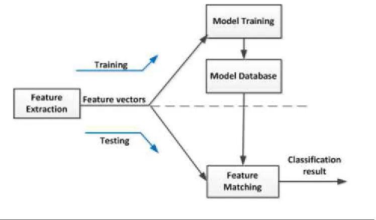
Like many other pattern classification tasks, audio classification is made up of three

fundamental components: (1) Sensing component - for measuring the sound event or

signal;(2) audio processing component - for extracting the characteristic features of the

measured sound signal; and (3) classification component - for recognition of the context

of the sound event.

In audio based CA applications, the sensing (measurement) is normally done using

microphones. The audio signal processing part mainly deals with the extraction of

features from the recorded audio signal. The various methods of time-frequency analysis

developed for processing audio signals, in many cases originally developed for speech

processing, are used. That is feature extraction quantizes the audio signal and transforms

it into various characteristic features. This results inn dimensional feature vector often

representing each audio frame. A classifier then takes this feature vector and determines

what it represents - that is, it determines context of the audio event.

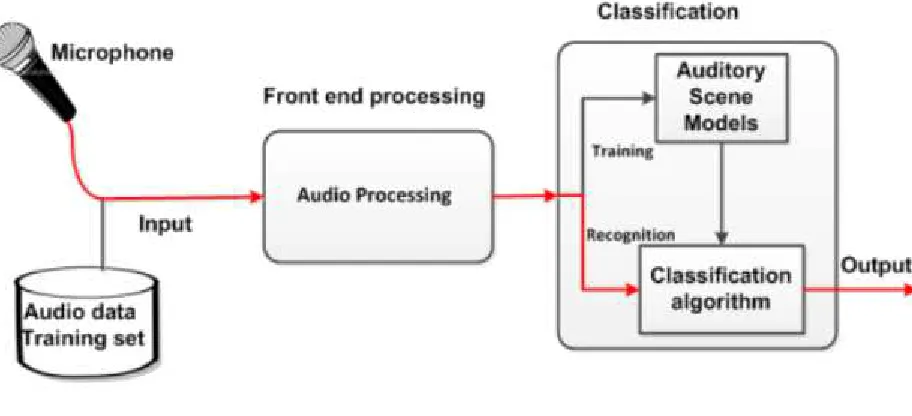
Figure1.1shows the general architecture of the audio classification system. In the figure,

input represents the raw audio data whereas output represents the activity (context)

[image:19.596.112.568.472.680.2]

information.

(20)

The ESR technique has two phases: training phase and recognition phase. During

the training phase the system receives its inputs from pre-recorded audio data training

sets and generates representative models for each of the audio event/scene. On the

other hand, during the recognition phase, the system receives its audio inputs directly

from the smartphone’s microphone. The recognition phase uses the models generated

during the training phase for matching and determining the type of audio received by

the microphone. The recognition phase processes the audio data online and in-time

without delay in order to deliver continuous and real-time recognition output for the

user. Detailed discussion about the process and steps of the ESR technique is provided

in chapter 5(design procedures).

The following are the main procedures that have been followed during the design of the

ESR/CA technique.

1. First, thorough literature study of (state-of-the-art) audio feature extraction

tech-niques and classification algorithms is conducted. The main goal of the preliminary

literature study is to pre-select the best set of audio feature and classification

al-gorithm combinations that can provide the highest possible recognition accuracy

with less computational complexities. This step is performed during the research

topic study (literature study)1

2. Offline test/simulation is performed in order to compare the performance of each

of the pre-selected techniques and then select the best one. Unlike speech and

music recognition, the research on environmental sound recognition (ESR) is not

yet well matured. It is still at its infant stage which makes it difficult to obtain

standard procedures and well organized information to determine the best audio

feature extraction techniques and classification algorithms, based solely on the

literature study. As a result, it is imperative to make further experimental test

and simulations in order to be able to determine the best techniques. All the

experimental simulations and comparison are performed first offline using Matlab

codes. The simulation results compare the performances of audio features and

classification algorithms based on their recognition accuracy and computational

speed (complexity). The offline simulation result is discussed in chapter6in detail.

1

(21)

3. Mobile application is developed using the best audio feature extraction and

classi-fication techniques chosen based on the Matlab (offline) simulation result, during

the Matlab experiment(step 3). The mobile application processes the audio data

online and provides real-time classification results. The developed mobile

applica-tion is discussed in chapter7.

The rest of the thesis is organized as follows: In chapter 2, we present a background

information in order to understand the basics and principles of digital audio signal

pro-cessing. Chapter3and chapter4, respectively, introduce audio features and classification

methods which are used in the thesis. In chapter5, we discuss the design procedures and

steps of the thesis project in detail. The chapter discusses each steps and components of

the ESR technique. Then chapter 6 provides the simulation results and analysis of the

results. In this chapter, the performance of the different classifiers are first presented

and compared in order to choose the best classifier. Then the performance of different

audio features is computed and compared in order to reduce feature dimension and to

choose the best feature set. Chapter7 discuss the development of Android application

and realization of the ESR technique on smartphone. Finally, in chapter8, we provide

(22)

(23)

Chapter 2

Background and Principles Used

This chapter provides a brief background information and basic principles and techniques

used in digital audio signal processing and analysis.

2.1 Digital Audio Analysis

The classical method of signal analysis, at spectral level, is based on classical Fourier

analysis to the whole signal. However, an exact definition of Fourier transform cannot be

directly applied in audio signal analysis because audio signals are time-varying signals

(non-stationary) in the real world and, indeed, all their meaning is related to such time

variability. Therefore, it is important to develop sound analysis techniques that allow

to grasp at least some of the distinguished features of time-varying sounds, in order to

ease the tasks of audio analysis such as feature extractions.

To solve these problems, audio signal is first split into a sequence of short segments,

called frames, in such a way that each one is short enough to be considered

pseudo-stationary. This process of dividing audio signal into frames is known as Framing. The

length of each frame ranges between 10 and 50ms (in such a short time period it is

assumed that the audio signal will not able to significantly change). Audio processing

(e.g., Fourier transform, feature extraction, etc...) is done frame by frame basis. Usually,

we multiply the frames with a smoothening functions such as Hamming window function

in order to eliminate sharp corners and discontinuities before we apply Fourier transform

operations on the frames. This process is called Windowing.

(24)

Chapter 2. Background: Principles of Digital Audio Analysis 12

The process of frame by frame analysis is known as short-time signal analysis. In the

literature there are variety of short-time analysis techniques such as Short-Time Fourier

Transform (STFT), Discrete Wavelet Transform (DWT) and Wigner distribution (WD)

[16]. STFT is the most popular short time analysis technique due to its computational

simplicity. In this section, we present short-time Fourier transform (STFT). Special

attention is reserved on criteria for choosing the analysis parameters, such as window

length and type.

2.1.1 Short-Time Fourier Transform

The Short-Time Fourier Transform (STFT) is nothing more than Fourier analysis

per-formed on slices of the time-domain signal. It performs Fast Fourier Transform (FFT)

analysis on short windows in time. This is also called “sliding-window” FFT. The

re-sults of the FFT represent the contents of the audio signal in terms of time-frequency

information. We analyze sound using STFT primarily because:

• It is simpler for time varying (non-stationary) signal processing and analysis.

• Enables us to represent the spectra of signals with spectral profiles that change over time.

• It allows adaptive and other non-linear signal modifications.

• Time-Frequency (T-F), i.e, STFT analysis is what the human brain does.

• It allows processing and signal modification directly in the Time-Frequency domain

In STFT the signal to be analyzed or transformed is broken up into a series of chunks

called frames, which usually overlap with each other, to reduce artifacts at the boundary.

The overlapping is also useful when the sample size of the training data is relatively

small. A set of training data produces more instances with a higher percentage of

overlapping than the same training data with a lower percentage of overlapping. Then

Fourier transform operation is then applied to successive frames. In other words, we

can think of STFT as multiplying audio signal x n

by a short-time window that is

centered around the time frame n. The segment of the signal contained in the window

(25)

of the Time-Frequency representation at a set of discrete frequencies. Equation 2.1

provides the mathematical definition of STFT.

Xm k

=

∞

X

n=−∞

x n

.w m−n

.e−j2_πnk/N

(2.1)

where

x n

= input signal at time n

w n

= length m window function (e.g., Hamming)

Xm k

= DTFT of windowed data (frame) centered about time n.

In practice, we need to compute the STFT on a finite set of N points. In what follows

we assume that the window is m ≤N samples long and N size input audio signal, so that we can use the DFT onN points, thus obtaining a sampling of the frequency axis

between 0 and 2π in multiples of 2π/N. The kth point in the transform domain (said

thekth _{bin of the DFT) is given by}

Xm k

=

N−1

X

n=0

x n

.w m−n

.e−j2_πnk/N

(2.2)

If we assumeP to be the overlap size (in terms of number of samples) between successive

frames, then we can compute the number of frames as follows:

N umber of f rames=b N −m

/P

c+ 1 (2.3)

where b c is a symbol for rounding down a fraction value to the nearest integer value, known as flooring.

2.1.2 Commonly Used Windows

We have already seen that audio analysis methods (such as the STFT) first divide the

input audio signal into smaller time segments, or frames. Audio classification algorithms

are then applied separately to each frame. The classification result of each frame is then

(26)

In the literature, three different framing techniques have been used for audio analysis:

sliding windows, event-defined windows and activity-defined windows [17]. With the

sliding window method, the signal is divided into windows of fixed length with no

inter-window gaps. A range of inter-window sizes have been used in previous studies from 0.25 s [18]

to 6.7 s [19], with some studies including a degree of overlap between adjacent windows

[19,20]. The sliding window approach does not require pre-processing of the sensor signal

and is therefore ideally suited to real-time applications. Due to its implementational

simplicity, most audio analysis and classification studies have employed this approach.

Thus, we use sliding window in our implementation for dividing or splitting the input

audio signal into smaller time segments, or frames. Then the frame is multiplied (filtered)

with window functions such as Hanning or Hamming functions in order to eliminate

boundary discontinuities.

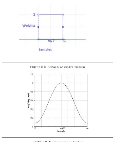
The two commonly used windows are rectangular window and Hamming window:

• The rectangular window- Rectangular window is the simplest analysis win-dow. In fact, the framing process using a rectangular sliding window results in

already rectangularly windowed signal. Therefore, further windowing process is

not required in the case of windowing audio signal using rectangular window. The

rectangular window is mathematically defined as

wR n

=     

1 n= 1, ..., m−1

0 elsewhere

(2.4)

wherem is the window size (in terms of number of samples)

Figure 2.1provides the shape of the rectangular window.

• Hamming window- Widowing using Hamming window is performed by simply multiplying the framed signals with the Hamming window. Usually, the framed

signal and the Hamming window used has equal size. The Hamming window is

mathematically defined as

wH n= 0.54−0.46cos

2π n−1

m−1

,1≤n≤m (2.5)

(27)

[image:27.596.119.518.67.556.2]

Figure 2.1: _{Rectangular window function}

Figure 2.2: _{Hamming window function}

2.1.3 Selection of windowing parameters

There are three main windowing parameters that can affect the result of the STFT:

window type (shape), window size and ovelapping size (hop size). Next, we examine the

effect of each of the parameters on the STFT.

• Window type- The rectangular window (i.e., no windowing) can cause prob-lems when we do Fourier analysis; it abruptly cuts of the signal at its boundaries

[image:27.596.182.439.78.245.2]

(28)

window function has a narrow main lobe and low side lobe levels in their

trans-fer functions, which shrinks the values of the signal toward zero at the window

boundaries, avoiding discontinuities. As a result, Hamming window is preferably

used for windowing purposes over rectangular window.

• Window size- We have discussed different motivations for splitting audio into segments for processing. However, we did not consider how big those segments,

frames, or analysis windows should be. There are two main important factors that

has to be considered for determining the window size; i.e, signal stationarity and

time-frequency resolution.

Signal stationarity- Fast Fourier transform (FFT) operation assumes that the

fre-quency components of the signal are unchanging (i.e, stationary– in fact,

pseudo-stationary) across the analysis window of interest. Any deviation from this

as-sumption would result in inaccurate determination of the frequency components.

This point reveals that the importance of ensuring that the analysis window

lead-ing to FFT is sized so that the signal is stationary across the period of analysis.

In practice, many audio signals do not tend to remain stationary for so long, and

thus smaller analysis window are necessary to capture the rapidly changing details.

Many literature assume audio signal to be stationary (pseudo-stationary) over a

period of about 20 – 50 ms.

Time-frequency resolution- Moving back to FFT, the output frequency vector,

from anN-sample FFT of audio signal sampled atFs Hz, contains N

2 + 1 positive frequency bins. Each bin collects the energy from a small range of frequencies

in the original signal. The bin width is related to both the sampling rate and

to the number of signals being analysed, Fs

N. Put another way, this bin width is

equal to the reciprocal of the time span encompassed by the analysis window. It,

therefore, makes sense that in order to achieve a higher frequency resolution, we

need to collect a longer duration of samples. However, for rapidly changing signals,

collecting more of them means we might end up missing some time domain features

as we have discussed above.

So the window length (size) is chosen according to the trade-off between higher

frequency/spectral resolution (more samples) and time/temporal resolution (less

samples) governed by the uncertainty principle. Smaller window width results in

(29)

analysis is based on the assumption that, within one frame, the signal is stationary.

The shorter the window, the more true the assumption is. However, short windows

result in low spectral/frequency resolution. Thus, the choice of analysis window

size depends on the requirement of the problem. (Discrete) Wavelet Transform

(DWT) and Wigner distribution (WD) [16] are used as alternatives to STFT in

order to satisfy the demand of both high frequency and time resolutions. However,

these methods are more computationally intensive compared to STFT. The main

limitation of STFT is that it has a fixed time-frequency resolution due to the fixed

window size used.

• Window overlapping size

Overlapping ensures that audio features occurring at a discontinuity are at least

considered whole in the subsequent overlapped frame. The degree of overlap

(usu-ally expressed as percentage) describes the amount of previous frame that is

re-peated in the following frame. Overlap of 25% and 50% are common. Similar to

the window size, the determination of the overlap size depends very much on the

purposes of the analysis or application. In general, more overlap will give more

analysis points and therefore smoother results across time which can possibly lead

to better recognition accuracy, but the computational expense is proportionately

(30)

(31)

Chapter 3

Audio Features

Audio features can be broadly classified based on their semantic interpretation as

percep-tual and physical features. Perceppercep-tual features approximate properties that are perceived

by human listeners such as pitch, loudness, rhythm, and timbre. In contrast, physical

features describe audio signals in terms of mathematical, statistical, and physical

prop-erties. Based on the domain of representation, physical features are further divided as

temporal features and spectral features. In this chapter, we introduce various physical

features that are used during the implementation of this project. These audio features

have been selected as the most appropriate features for ESR applications based on the

literature survey that has been performed during the research topic study 1

. However,

before we present the audio features, it is important to, first, look into the criteria we

used in order to select the audio features.

3.1 Requirements for Audio Features Selection

In the literature, there are a number of audio feature extraction techniques. The

recogni-tion accuracy and performance of the ESR is highly affected by the type of audio feature

extraction techniques that are used. As a result, a wise selection of audio features and

classifiers is important in order to obtain a good (acceptable) performance and

recog-nition accuracy. The type of audio feature one selects depends mainly on the type and

purpose of the application one wants to use. The assumption is that the audio based CA

1

title ‘Audio based context awareness system using smartphones’

(32)

Chapter 3. Audio Features 20

technique (ESR) will be implemented on a resource constrained devices such as smart

mobile phones. The requirements for implementation of such applications include low

computational complexity and power consumption. However, these requirements often

affect the recognition accuracy of the ESR as well. Therefore, the selection of the audio

features should be done with the main goal of developing a CA technique which has low

computational complexity, energy consumption, memory requirement, and yet provides

acceptable recognition accuracy. The following are some of the parameters that have

been used, whenever possible, to select the audio features.

• Small feature size- Large feature size leads to high computational cost and curse of dimensionality . Thus, it is important to reduce the number of features,

for example, by avoiding redundancies in the feature space. On the other hand,

using smaller feature size may result in reduced classification accuracy. Thus, it is

important to select an audio feature with optimum feature size that can provide

an acceptable level of accuracy and performance as well as reduced computational

cost.

• Low computational complexity- The computational complexity of an audio feature refers to the amount of computation time required to produce the audio

feature. Audio features that require lower computation time are preferred to audio

features that require higher computation time.

• High inter-class variability-Achieving increased discrimination among different classes of audio patterns is crucial for increased recognition accuracy. Inter-class

variability refers to discrimination power of audio feature across different classes.

Therefore, good audio features should show high inter-class variability.

• High intra-class similarity- Decreased discrimination among similar classes or sound events belonging to same class is crucial for increased recognition accuracy.

Consequently, audio features extracted from sound events or environmental sounds

belonging to a similar class should have similar behavior or should not show

sig-nificant deviation among each other.

• Low sensitivity- An indicator for the robustness of a feature is the sensitivity to minor changes in the underlying signal. Usually, low sensitivity is desired in order

(33)

3.2 Audio Physical Features

Unlike the perceptual features which can only perceived by human being, physical

fea-tures refers to physical quantities that can be measured or computed using mathematical

formulations. In some literatures, physical features are further divide into three groups

as temporal, spectral and cepstral features. However, most of the literatures categorize

physical audio features into temporal and spectral features. In the later case, there is

no distiniction between the cepstral domain features and the spectral domain features.

They are considered as the same domain with common group name, spectral domain

features. We adopt the later grouping method for simplicity purposes (temporal and

spectral features).

3.2.1 Temporal Features

The temporal domain is the native representation domain for audio signals. All

tem-poral features are extracted directly from the raw audio signal, without any preceding

transformation. Consequently, the computational complexity of temporal features tends

to be low compared with that of the spectral features.

Temporal features of audio signal includes:

• Zero crossing rate (ZCR)- ZCR is the most common type of zero crossing based audio features [21]. It is defined as the number of time-domain zero crossings within

a processing frame. It indicates the frequency of signal amplitude sign change.

ZCR allow for a rough estimation of dominant frequency and spectral centroid

[22]. We used the following equation to compute the average zero-crossing rate.

ZCR= 1 2N

N

X

n=1

|sgn x n

−sgn x n−1 |

(3.1)

where x is the time-domain signal, sgn is the signum function, and N is the size

of processing frame. The signum function implementation can be defined as

sgn x =     

1 x≥0

−1 x <0

(34)

One of the most attractive properties of the ZCR is that it is very fast to calculate.

As being a time-domain feature, there is no need to calculate the spectra.

Fur-thermore, a system which uses only the ZCR-based features would not even need

digital-to-analog conversion, but only the information whenever the sign of the

signal changes. However, ZCR can be sensitive to noise. Though using a threshold

value (level) near to zero can significantly reduce the sensitivity to noise,

deter-mining appropriate threshold level is not easy.

• Short-time energy (STE) – The short-time energy [23] is one of energy based audio features. Li [24] and Zhang [25] used it to classify audio signals. It is easy to

calculate and provides a convenient representation of the amplitude variation over

time. It indicates the loudness of an audio signal. STE is a reliable indicator for

silence detection. It is defined to be the sum of a squared time domain sequences

of audio data, as shown in equation 3.3.

ST E = 1

N N

X

n=1

x n2

(3.3)

wherex n

is the value of the sample (in time domain) andN is the total number

of samples in the processing window (frame size). The STE of audio signal may

be affected by the gain value of the recording devices. Usually we normalize the

value of STE to reduce the effect.

ZCR and STE are widely used in speech and music recognition applications [26]. Speech,

for example, has a high variance in ZCR and STE values, while in music these values are

normally much more constant. ZCR and STE have been also used in ESR applications

[27] due to their simplicity and low computational complexity.

• Temporal centroid (TC) -TC is the time average over the envelope of a signal in seconds [28]. It is the point in time where most of the energy of the signal is

located in average.

T C=

PN

n=1n.|x n

|2

PN

n=1|x n

|2 (3.4)

Note that the computation of temporal centroid is equivalent to that of spectral

(35)

• Energy entropy (EE)- The short-term entropy of energy can be interpreted as a measure of abrupt changes in the energy level of an audio signal. In order to

compute it, we first divide each short-term frame inKsub-frames of fixed duration.

Then for each sub-frame,j, we compute its energy as in Eq. (3.3). and divide it by

the total energy, EshortF ramei, of the short-term frame. The following equations

presents the procedure to compute the energy entropy of a frame (short-term

frame).

ej =

EsubF ramej

EshortF ramei

(3.5)

where

EshortF ramei =

K

X

k=1

EsubF ramek. (3.6)

At a final step, the entropy,H(i), of the sequenceej is computed according to the

equation:

H(i) =−

K

X

j=1

ej.log2(e_j). (3.7)

• Autocorrelation (AC)-The autocorrelation domain represents the correlation of a signal with a time-shifted version of the same signal for different time lags

[21]. It reveals repeating patterns and their periodicities in a signal and can be

employed, for example, for the estimation of the fundamental frequency of a signal.

This allows distinguishing between sounds that have harmonic spectrum and

non-harmonic spectrum, e.g., between musical sounds and noise. Autocorrelation of a

signal is calculated as follows:

AC =fxx[τ] =x[τ]∗x[−τ] = N−1

X

n=0

x n

.x n+τ

(3.8)

whereτis the lag (discrete delay index),fxx[τ] is the corresponding autocorrelation

value, N is the length of the frame n the sample index, and when τ = 0, fxx[τ]

becomes the signal’s power. Similar to the way RMS is computed, autocorrelation

also steps through windowed portions of a signal where each windowed frame’s

samples are multiplied with each other and then summed according to the above

equation. This is repeated where one frame is kept constant while the otherx n+

τ

(36)

• Root mean square (RMS)- As STE, the RMS value is a measurment of energy in a signal. The RMS value is however defined to be the square root of the avaerage

of a squared signal, as seen in equation3.9.

RM S = v u u t 1 N N X n=1

x n2

(3.9)

3.2.2 Audio Spectral Features

The group of frequency domain features is the largest group of audio features. The

frequency domain reveals the spectral distribution of a signal. For each frequency (or

frequency band/bin) the domain provides the corresponding magnitude and phase. Since

phase variation has little effect on the sound we hear, features that evaluate the phase

information are usually ignored. Consequently, we focus on features that capture basic

properties of the spectral properties of audio signal: subband energy ratio, spectral

flux, spectral centroid, spectral entropy, spectral roll-off, and Mel-frequency cepstral

coefficients (MFCCs).

Popular transformations from time to frequency domain are Discrete Fourier Transform

(DFT), Discrete Cosine Transform (DCT), and Discrete Wavelet Transform (DWT).

Another widely-used way to transform a signal from temporal to frequency domain is

the application of banks of band-pass filters with e.g. Mel and Bark-scaled filters to the

time domain signal. However, discrete Fourier transform is widely used for its simpler

computational complexities. Next we introduce spectral audio features that are used in

our environmental audio based context recognition application.

• Spectral centroid(SC)- Spectral centroid [21] represents the “balancing point”, or the midpoint of the spectral power distribution of a signal. It is related to

the brightness of a sound. The higher the centroid, the brighter (high frequency)

the sound is. A spectral centroid provides a noise-robust estimate of how the

dominant frequency of a signal changes over time. As such, spectral centroids

are an increasingly popular tool in several signal processing applications, such

as speech processing. Spectral centroid is obtained by evaluating the “center of

gravity” using the Fourier transform’s frequency and magnitude information. The

(37)

by amplitudes, divided by the sum of the amplitudes. The following equation shows

how to compute the spectral centroid, SCi, of theith audio frame.

SCi =

PK−1

k=0 k.|Xi k

|2

PK−1

k=0 |Xi k

|2 (3.10)

Here, Xi(k) is the amplitude corresponding to bin k (in DFT spectrum of the

signal) of the ith _{audio frame and} _K _{is the size of the frame. The result of the}

spectral centroid is a bin index within the range 0 < SC < K −1. It can be converted either to Hz (using equation 3.11 ) or to a parameter range between

zero and one by dividing it by the frame size,K. The frequency of bin indexk can

be computed from the block (frame) lengthK and sample ratefs by:

f k = fs

K

k (3.11)

Low results indicate significant low frequency components and insignificant high

frequency components (low brightness) and vice versa.

• Spectral spread (SS)- The spectral spread is the second cental moment of the spectrum. It is a measure that signifies if the power spectrum is concentrated

around the centroid or spread out over the spectrum. In order to compute it, one

has to take the deviation of the spectrum from the spectral centroid, according to

the following equation:

SCi =

v u u t

PK−1

k=0 (k−SCi) 2_._|_X

i k|2

PK−1

k=0 |Xi k

|2 (3.12)

• Spectral rolloff point (SRP)- The spectral rolloff point is the N% percentile of the power spectral distribution, where N is usually 85% or 95% [29]. The spectral

rolloff point is the frequency below which N% of the magnitude distribution is

concentrated. It increases with the bandwidth of a signal. Spectral rolloff is

ex-tensively used in music information retrieval [30] and speech/music segmentation.

The spectral rolloff point is calculated as follows:

SRP =f N

where f N = fs

K

(38)

whereN is the largest bin that fulfills equation3.14.

N

X

k=0

|X(k)|2

≤T H. K−1

X

k=0

|X(k)|2

(3.14)

where X(k) are the magnitude components, k frequency index and f(K) (the

fre-quency) spectral roll-off point with 100∗T H

% of the energy. TH is a threshold

between 0 and 1. A commonly used value for the threshold is 0.85 and 0.95

[29, 31]. This measure is useful in distinguishing voiced speech from unvoiced:

unvoiced speech has a high proportion of energy contained in the high-frequency

range of the spectrum, whereas most of the energy for voiced speech and music is

contained in lower bands [32].

• Spectral flux (SF)- The SF is a 2-norm of the frame-to-frame spectral amplitude difference vector. It defines the amount of frame-to-frame fluctuation in time. i.e.,

it measures the change in the shape of the power spectrum. It is computed via

the energy difference between consecutive frames as follows:

SFf = K−1

X

k=0

||Xf k| − |Xf−1 k

|| (3.15)

where f is the index of the frame and K is the frame length. Spectral flux is

an efficient feature for speech/music discrimination, since in speech the frame-to

frame spectra fluctuate more than in music, particularly in unvoiced speech [33].

• Spectral entropy (SE)- Spectral entropy [34] is computed in a similar manner to the entropy of energy, although, this time, the computation takes place in the

frequency domain. More specifically, we first divide the spectrum of the short-term

frame intoLsub-bands (bins). The energyEf of thefthsub-band,f = 0, ..., L−1,

is then normalized by the total spectral energy, thst is, nf =

Ef

PL−1

f=0Ef

, f =

0, ..., L−1.The entropy of the normalized spectral energynf is finally computed

according to the equation:

H=−

L−1 X

f=0

nf.log2(n_f) (3.16)

(39)

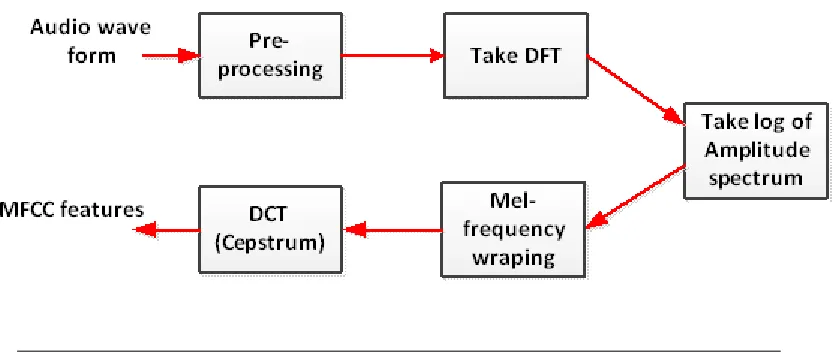
[image:39.596.117.534.205.382.2]

domains of audio recognition applications such environmental sound classifications

[27, 51, 52]. They represent timbral information (spectral envelop) of a signal.

Computation of MFCC includes conversion of the Fourier coefficients to Mel-scale.

After conversion, the obtained vectors are logarthmized, and decorrelated by

dis-crete cosine transform (DCT) in order to remove redundant information. Figure

3.1shows the process of MFCC feature extraction.

Figure 3.1: _{MFCC extraction process}

In figure3.1, the first step, preprocessing, consists of pre-emphasizing, frame

block-ing and windowblock-ing of the signal. The aim of this step is to model small (typically,

20ms) sections of the signal (frame) that are statistically stationary. The window

function, typically a Hamming window, removes edge effects. The next step takes

the Discrete Fourier transform (DFT) of each frame. We retain only the logarithm

of the amplitude spectrum. We discard phase information because perceptual

studies have shown that the amplitude of the spectrum is much more important

than the phase. We take the logarithm of the amplitude because the perceived

loudness of a signal has been found to be approximately logarithmic. After a

discrete Fourier transform, the power spectrum is transformed to Mel-frequency

scale. This step smooths the spectrum and emphasizes perceptually meaningful

frequencies. Mel- frequency scale is based on mapping between actual frequency

and perceived pitch by human auditory system. The mapping is approximately

linear below 1 KHz and logarithmic above. This is done by using a filter bank

(40)

conversion between a frequency value in Hertz (f) and in mel is given by:

mel f

= 2595log10 1 +

f

700

(3.17)

Finally, the cepstral coefficients are calculated from the mel-spectrum by taking

the discrete cosine transform (DCT) of the logarithm of the mel-spectrum. This

calculation is given in by:

ci = K−1

X

k=0

(logSk).cos iπ K k−

1 2

(3.18)

where ci is the ith MFCC, Sk is the output of kth filter bank channel (i.e. the

weighted sum of the power spectrum bins on that channel) and K is the number

of coefficients (number of Mel-filter banks). The value ofK used is mostly between

20 to 40. In this project we used the value of K to be equal to 23.

The components of MFCCs are the first few DCT coefficients that describe the

coarse spectral shape. The first DCT coefficient represents the average power

(energy) in the spectrum. The second coefficient approximates the broad shape of

the spectrum and is related to the spectral centroid. The higher order coefficients

represent finer spectral details (e.g., pitch). In practice, the first 8-13 MFCC

coefficients are used to represent the shape of the spectrum. The higher order

coefficients are ignored since they provide more redundant information. However,

some applications require more higher-order coefficients to capture pitch and tone

(41)

Chapter 4

Audio Classifiers

Based on their learning behavior, classifiers can be divided into two groups:

classi-fiers that use supervised learning (supervised classification) and unsupervised learning

(unsupervised classification). In supervised classification, we provide examples of the

correct classification (a feature vector along with its correct class) to teach the

classi-fier. Based on these examples, which are commonly termed as training samples, the

classifier then learns how to assign an unseen feature vector to a correct class.

Exam-ples of supervised classifications include Hidden Markov Model (HMM)[35], Gaussian

Mixture Models (GMM)[36], K- Nearest Neighbor (k-NN)[35], Support Vector Machine

(SVM)[37], Artificial Neural Networks (ANN), Bayesian Network (BN)[35], and

Dy-namic Time Wrapping (DTW)[38]. In unsupervised classification or clustering, there is

neither explicit teacher nor training samples. The classification of the feature vectors

must be based on similarity between them based on which they are divided into natural

groupings. Whether any two feature vectors are similar depends on the application.

Obviously, unsupervised classification is a more difficult problem than supervised

clas-sification and supervised clasclas-sification is the preferable option if it is possible. In some

cases, however, it is necessary to use unsupervised learning. For example, this is the

case if the feature vector describing an object can be expected to change with time.

Ex-amples of unsupervised classifications include k-means clustering, Self-Organizing Maps

(SOM), and Linear vector Quantization (LVQ).

Classifiers can also be grouped based on reasoning process as probabilistic and

deter-ministic classifiers. Deterdeter-ministic reasoning classifiers classify sensed data into distinct

(42)

Chapter 4Audio Classifiers 30

states and produce a distinct output that cannot be uncertain or disputable.

Proba-bilistic reasoning, on the other hand, considers sensed data to be uncertain input and

thus outputs multiple contextual states with associated degrees of truthfulness or

prob-abilities. Decision of the class type to which the feature belongs is made based on the

highest probability.

4.1 Requirements for Audio Classifier Selection

The two main criteria that can be used to select classification techniques are

computa-tional complexity and recognition accuracy. Moreover, robustness to noise can be used

as a criteria in some applications; especially, in a noise prone application.

• Computational complexity- The computational complexity of a classifier can be measured by the amount of computational time it requires to produce the

classification result. Computational complexity of an algorithm can also provide

insight about its power consumption. It is preferred to use classifiers with low

computational complexity, which can provide classification result faster and as a

result consume less power.

• Recognition accuracy- The recognition accuracy of a classifier can be affected by a number of factors. Selection of audio feature is the most important factor that

affects the recognition accuracy. In addition, selection of a good type of classifier

improves the recognition accuracy.

• Robustness to noise- Any good classifier should be able to ignore any feature variations caused by disturbances such as noise, bandwidth or the amplitude

scal-ing of an audio signal.

Similar to the case of audio feature selection, the selection process of audio classifiers

usually requires a trade-off between computational complexity and recognition accuracy.

In the literature, there are many different audio classifiers. However, there is no

suffi-cient previous work that compares the performance of the audio classifiers based on the

above requirements. Thus, we select some classifiers based on their popularity and then

(43)

GMM are chosen due to their common use in a number of ESR applications/problems

for discussion (in this chapter) and further performance comparison (in chapter5).

4.2 Popular classifiers

We start description of selected classifiers with the famous k-nearest neighbor classifier

(k-NN classifier) and proceed with the gaussian mixture model (GMM) and the more

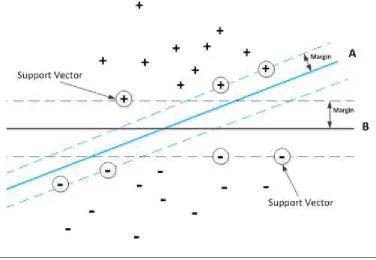
sophisticated support vector machines (SVMs). Obviously, this is just a very small

subset of the classifiers that have been proposed and studied in the literature but serve

well our purpose to focus on selected methods which are both popular and representative

of the wealth of techniques that are available. Lengthy theoretical descriptions of the

classifiers have been avoided and instead an attempt to highlight the key ideas behind

the algorithms being studied is made. These set of classifiers have been selected for

experimental and simulation test in our implementation due to their popular use in the

literature. We look into their applicability for mobile devices (smartphones) in chapter

6 taking into account the limited resources (like energy, cpu, memory) of the mobile

device. Chapter6 provides the performance comparison of the classifiers based on their

classification accuracy and computational speed.

4.2.1 The k-Nearest Neighbor Classifier (k-NN)

Despite its simplicity, the k-NN classifier is well tailored for both binary and multi-class

problems. Its outstanding characteristics is that it does not require a training stage in

the strict sense. The training samples are rather used directly by the classifier during

the classification stage. The key idea behind this classifier is that, if we are given a set

of patterns (unknown feature vector), X, we first detect its k-nearest neighbors in the

training set and count how many of those belong to each class. In the end the feature

vector is assigned to the class which has the highest number of neighbors. Therefore,

for the k-NN algorithm to operate the following ingredients are required:

1. A data set of labeled samples, that is a training set of feature vectors and respective

class labels.

(44)

3. A distance (dissimilarity ) measure.

Let us now go through the k-NN algorithm in more detail. In the first step, the algorithm

computes the distance, d X, Vi, between X and each vector Vi, i = 1, ..., M, of the

training set, whereM is the total number of training samples. The most common choice

of distance measure is the Euclidian sistance, which is computed as:

d X, Vi = v u u t D X j=1 X j

−Vi j )2

(4.1)

where D is the dimentionality of the feature space. Another popular choice of distance

measure is known as the Mahalanobis distance [39]. Afterd X, Vi has been computed

for each Vi, the resulting distance values are sorted in ascending order. As a result, the

k first values correspond to thek closest neighbors of the unknown feature vector. Now,

let ki be the number of the training vectors among the k neighbors of X that belong

to the ith _class, _i_{= 1}_{, ..., N}

c. The unknown vector is then classified to the class which

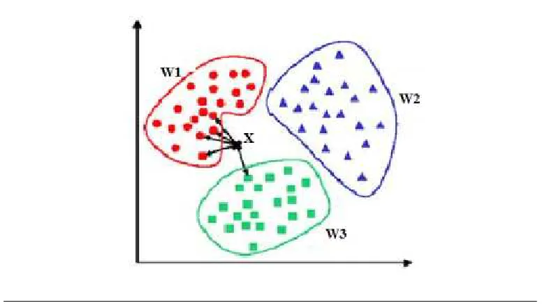
corresponds to the maximum ki. In the example in Figure 4.1 , we have three classes

and the goal is to find a class label for the unknown exampleX . The Euclidean distance

is used and k=5. Of the 5 closest neighbors, 4 belong to W1 and 1 belongs to W3 , so

X is assigned toW1, the predominant class.

It is important to note that the k-NN classifier can operate directely in a multi-class

environment. This is because its algorithmic steps are not restricted by the number of

classes that are involved.

The performance of the k-NN has been extensively studied in the literature. An

inter-esting theoretical finding is that ifk→ ∞, M → ∞, and k

M →0, then the classification

error approaches the Bayesian error [39]. In other words, if both k and M approach

infinity and k is infinitely smaller thanM, then thek-NN classifier tends to behave like

the optimal (Bayesian) classifier eith respect to the classification error.

The larger the dataset, the more satisfactory of the performance of thek-NN algorithm.

Concerning parameterk (the number of neighbors), it can be stated that the value ofk

is tuned after experimentation with the dataset at hand . In general, small values are

prefered by also taking into account the size of the dataset (so that k

M remains as small

(45)

[image:45.596.123.511.94.315.2]

Figure 4.1: _{k-NN Classification Example}

Another important issue is the computational complexity of the k-NN classifier which

can be prohibitively high when the volume of the dataset is really large (mainly due to

the number of Euclidian distances that need to be computed). Over the years, several

remedies to this computational issue have been proposed in the literature, e.g. [40,41].

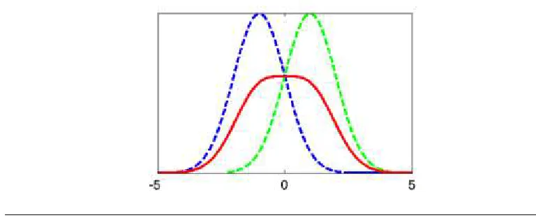
4.2.2 Gaussian Mixture Model (GMM)

The Gaussian Mixture Model (GMM) [42] is used in classifying different audio classes.

It is an example of a parametric classifier. It is an intuitive approach when the model

consists of several Gaussian components, which can be seen to model acoustic features.

In classification, each class is represented by a GMM and refers to its model. Once the

GMM is trained, it can be used to predict which class a new sample probably belongs

to [43].

The probability distribution of feature vectors is modeled by parametric or non-parametric

methods. Models which assume the shape of probability density function are termed

parametric. In non-parametric modeling, minimal or no assumptions are made

regard-ing the probability distribution of feature vectors. The potential of Gaussian mixture

models to represent an underlying set of acoustic classes by individual Gaussian

An environmental audio based context recognition system using smartphones

University of Twente