Permanent WRAP URL:
http://wrap.warwick.ac.uk/110843/
Copyright and reuse:
This thesis is made available online and is protected by original copyright.
Please scroll down to view the document itself.
Please refer to the repository record for this item for information to help you to cite it.
Our policy information is available from the repository home page.
HIGH RESOLUTION, HIGH SENSITIVITY TANDEM
MASS SPECTROMETRY OF MACROMOLECULES
USING TIME-OF-FLIGHT TECHNIQUES.
Emmanuel N. Raptakis
Submitted for the qualification of Doctor o f Philosophy.
University of Warwick.
Department of Chemistry
Title page... i
Table of Contents... ii
List of Figures...vii
Acknowledgments... xiv
Declaration... xv
Abbreviations... xvi
Abstract... xxiii
1. Chapter One...1
1.1 Evolution o f mass spectrometry and its applications... 1
1.1.1 The dawn of mass spectrometry...1
1.1.2 Mass analysers...3
1.1.2.1 Sector mass analysers... 3
1.1.2.2 Time-of-flight mass spectrometry... 7
1.1.2.2.1 Linear time-of-flight mass spectrometers...7
1.1.2.2.2 Historical overview...9
1.1.2.3 Ion reflectron in time-of-flight mass spectrometry... 15
1.1.2.3.1.1 Single stage reflectrons...15
1.1.2.3.1.2 Double stage reflectrons...19
1.1.2.3.1.3 Quadratic field reflectrons...24
1.1.3 Ionisation techniques...32
1.1.3.1 Historical overview... 32
1.1.3.3 Laser desorption... 36
1.1.3.4 Matrix assisted laser desorption and ionisation (MALDI)...37
1.1.3.4.1 Matrices in M ALDI... 41
1.1.3.4.2 MALDI and time-of-flight mass spectrometry... 43
1.1.3.5 Electrospray ionisation... 47
1.1.4 Ion detectors... 49
1.2 Tandem mass spectrometry...52
1.2.1 Instrumentation in tandem mass spectrometry... 55
1.2.2 Collision-induced dissociation... 59
1.2.3 Post-source decay... 66
1.3 Mass spectrometry in biological analysis... 68
1.3.1 Biological macromolecules... 68
1.3.2 Peptides and proteins sequencing... 70
1.3.2.1 Standard techniques...70
1.3.2.2 Pure mass spectrometric techniques...71
2. Chapter Two...76
2.1 Introduction... 76
2.2 Instrumentation... 76
2.2.1 The vacuum chamber...76
2.2.2 The ion source... 80
2.2.2.1 The wobble probe... 83
2.2.2.2 Acceleration and ion collimation region... 86
2.2.2.3 Ion trajectory simulations... 89
2.2.2.4 Design and construction...95
2.2.3 The laser system and beam delivery optics... 98
2.2.3.1 The excimer and dye lasers...98
2.2.3.2 The optical components... 100
2.2.4 The ion detector... 101
2.3 Experimental...101
2.4 Results and discussion... 105
3.2 The CONCEPT 4-sector double focusing tandem mass spectrometer. .111
3.3 The MALDI source...113
3.3.1 The nitrogen laser... 113
3.3.2 The optical components... 114
3.3.3 Ion optics... 118
3.3.4 The electrostatic analyser... 120
3.3.5 The magnetic analyser... 120
3.3.6 The array detector... 122
3.4 Experimental results and discussion... 124
4. Chapter Four...130
4.1 Introduction... ... 130
4.2 The double-focusing mass spectrometer as the first stage o f a tandem mass spectrometer...135
4.2.1 Time and spatial aberrations in the two sectors...135
4.2.2 The ion buncher... 140
4.2.3 Time-of-flight aberrations on electrostatic lenses...146
4.3 The quadratic-field mirror as the second stage of a tandem mass spectrometer... 150
4.3.1 Theoretical considerations on resolution in an ideal-focusing mirror. 150 4.3.1.1 Fundamental limitations on mass resolution... 151
4.3.1.1.1 Length of field-free region...151
4.3.1.1.2 Limitations inherent to the fragmentation process... 156
4.3.1.1.2.1 Velocity spread caused by collision-induced dissociationl56 4.3.1.1.2.2 Limits to mass resolution due to the length of the collision cell...158
4.3.1.1.3 Metastable decay... 161
4.3.1.2 Comparison with the orthogonal scheme... 164
4.3.2.1 Ion transmission in the quadratic field... 167
4.3.2.2 Limits to transmission due to angular scattering...173
4.3.3 Beam deflector design... 174
5. Chapter Five...177
5.1 Overview...177
5.2 Ion production and transmission in the double-focusing analyser... 179
5.2.1 Design and construction o f a MALDI ion source for the Concept double-focusing mass spectrometer... 179
5.2.1.1 Ion source employing quadrupole doublet... 186
5.2.1.1.1 The extraction and collimation regions...189
5.2.1.1.2 The quadrupole doublet...192
5.2.1.2 Ion source employing electrostatic lenses... 197
5.2.2 The parallel tim e-of-flight analyser and intermediate detection system...202
5.3 Construction of the time-of-flight mirror of the Mag-TOF tandem mass spectrometer...204
5.3.1 Introduction and vacuum system... 204
5.3.2 The ion buncher and delivery ion optics... 206
5.3.3 The collision cell, post-accelerating region and z-deflector... 214
5.3.4 Design and construction o f the quadratic field mirror... 218
5.3.4.1 Multi-electrode system for sustaining the quadratic field...218
5.3.4.2 Long-range field sag and its correction...221
5.3.4.3 Short-range perturbations...223
5.3.4.4 Perturbations on the field boundaries...225
5.3.4.4.1 The front boundary of the ion mirror... 225
5.3.4.4.2 The end-electrode of the ion mirror... 227
5.3.5 Practical design considerations... 227
5.4 Control and acquisition system... 233
5.5 Results and discussion...237
5.5.1 Transmission optimization and alignment experiments...237
5.6 Conclusions...245
List of Figures
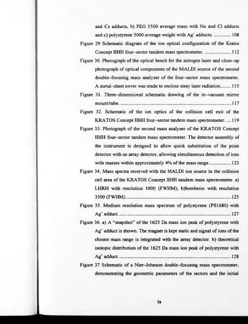
Figure 1. The diagram shows the operating principle of a “velocity focusing”
mass spectrograph similar to the one designed by Aston (see text)... 6
Figure 2. Schematic of the Willey-MacLaren time-of-flight mass spectrometer. 11
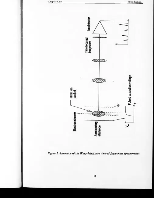
Figure 3. Schematic of a plasma desorption mass spectrometer...14
Figure 4. Schematic diagram showing the flight path of an ion in a
single-stage reflectron time-of-flight analyser... 17
Figure 5. Schematic of a time-of-flight mass spectrometer with a double stage
ion reflectron... 21
Figure 6. Ion flight times as a function of energy in a time-of-flight mass
analyser with a double-stage reflectron []... 23
Figure 7. Potential distribution in quadratic fields along the ion optical axis x<,
is the initial coordinate (starting point) o f an ion. 2a-Xd is the coordinate
of ideal time focusing... 25
Figure 8. Schematic o f the quadratic ion mirror time-of-flight instrument
introduced by Yoshida [37]...28
Figure 9. Assembly drawing of a time-of-flight instrument incorporating a
quadratic ion mirror. The quadratic potential distribution is created by
pure geometry field-sustaining electrodes... 31
Figure 10. Schematic of the VMASS time-of-flight mass spectrometer... 33
Figure 11. Schematic diagram of an L-SIMS ion source... 35
Figure 12. Positive ions MALDI spectra at 266 nm of bovine insulin with
sinapinic acid as matrix at various laser fluences. The energy of the
laser pulses is measured using a calibrated photodiode system []...40
Figure 13. Chemical compositions of some of the most widely used matrices
in MALDI mass spectrometry...45
Figure 14. An electron multiplier optimised for time-of-flight use. The first
dynode is perpendicular to the ion path to eliminate time-spread... 50
Figure 15. Schematic o f the KRATOS 4-sector tandem mass spectrometer. ..54
Figure 16. Schematic o f a triple-quadrupole tandem mass spectrometer... 56
Figure 19. Photograph and schematic diagram of the large scale time-of-flight
mass spectrometer...78
Figure 20. Mechanical drawing and photograph of the wobble probe... 84
Figure 21. SIMION ion trajectory simulations illustrating the effect of an
accelerating and a decelerating “Einzel” lens on the same diverging ion
beam. The two lenses have identical geometry. The decelerating lens
can achieve the same focusing conditions as the accelerating, for lower
values of potential...88
Figure 22. The ion source model as implemented in the SIMION software. ..90
Figure 23. A micro-lens created in the vicinity of the hole on the accelerating
electrode, may over-focus ions coming out of the sample surface for
certain electrode geometries and positions of the sample probe...92
Figure 24. SIMION simulations of ion trajectories in the chosen geometry for
the ion source of the large-scale time-of-flight mass spectrometer, (a)
accelerating lens, (b) decelerating lens...94
Figure 25. Assembly drawing of the ion source of the large-scale time-of—
flight mass spectrometer... 96
Figure 26. Time-of-flight mass spectrum of Csl clusters received in the large
scale TOF mass spectrometer. The resolution of this spectrum is 400
FWHM, although resolution of 700 has been observed for single shot
experiments... 103
Figure 27. a) MALDI mass spectrum of mixture of bombesin and bovine
insulin with sinapinic acid matrix, received in the large scale tim e-of-
flight mass spectrometer, b) MALDI mass spectrum of bombesin with
4—hydroxy a-cyanocynamic acid matrix, demonstrating matrix-adduct
peaks... 106
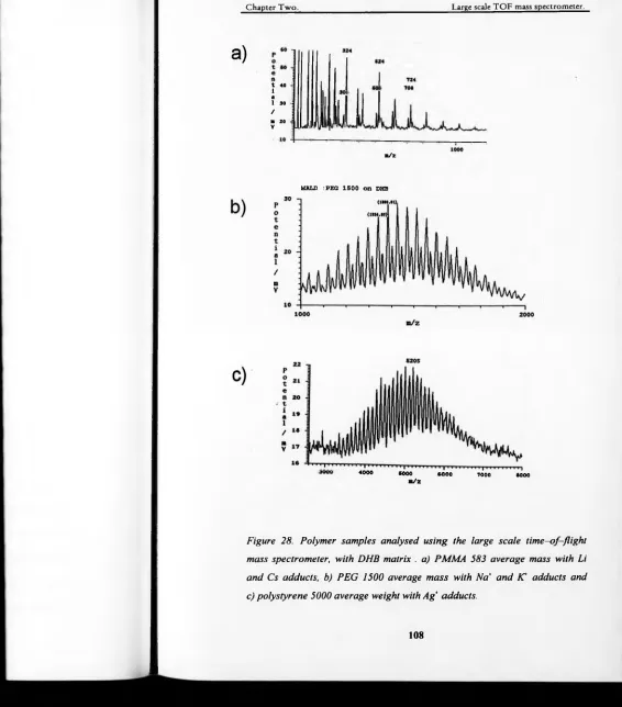
Figure 28. Polymer samples analysed using the large scale time-of-flight mass
and Cs adducts, b) PEG 1500 average mass with Na and Cl adducts
and c) polystyrene 5000 average weight with Ag* adducts...108
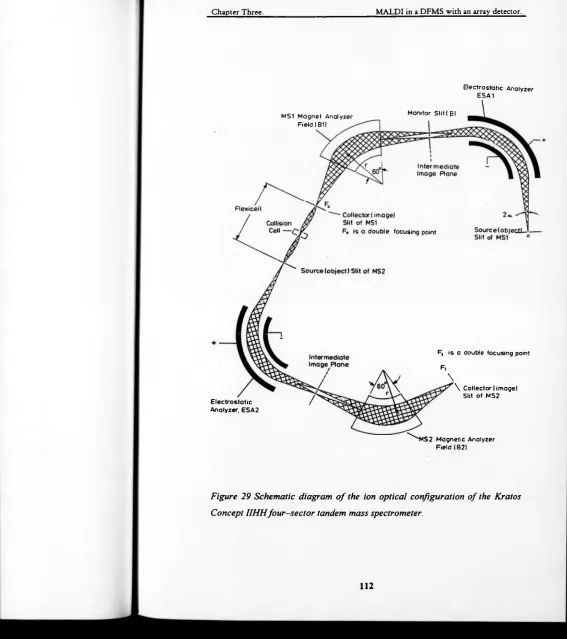
Figure 29 Schematic diagram of the ion optical configuration o f the Kratos
Concept IIHH four-sector tandem mass spectrometer... 112
Figure 30. Photograph o f the optical bench for the nitrogen laser and close-up
photograph of optical components of the MALDI source o f the second
double-focusing mass analyser of the four-sector mass spectrometer.
A metal-sheet cover was made to enclose stray laser radiation... 115
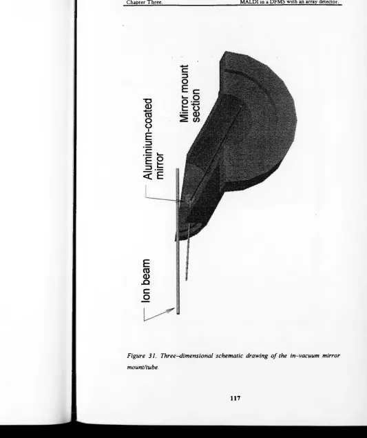
Figure 31. Three-dimensional schematic drawing of the in-vacuum mirror
mount/tube... 117
Figure 32. Schematic o f the ion optics of the collision cell exit of the
KRATOS Concept IIHH four-sector tandem mass spectrometer...119
Figure 33. Photograph of the second mass analyser of the KRATOS Concept
IIHH four-sector tandem mass spectrometer. The detector assembly of
the instrument is designed to allow quick substitution of the point
detector with an array detector, allowing simultaneous detection of ions
with masses within approximately 4% of the mass range... 123
Figure 34. Mass spectra received with the MALDI ion source in the collision
cell area o f the KRATOS Concept IIHH tandem mass spectrometer, a)
LHRH with resolution 1000 (FWHM); b)bombesin with resolution
3500 (FWHM)... 125
Figure 35. Medium resolution mass spectrum of polystyrene (PS1680) with
Ag* adduct...127
Figure 36. a) A “snapshot” of the 1625 Da mass ion peak of polystyrene with
Ag* adduct is shown. The magnet is kept static and signal of ions of the
chosen mass range is integrated with the array detector, b) theoretical
isotopic distribution of the 1625 Da mass ion peak of polystyrene with
Ag* adduct...128
Figure 37 Schematic of a Nier-Johnson double-focusing mass spectrometer,
demonstrating the geometric parameters o f the sectors and the initial
[image:10.638.76.562.17.652.2]Figure 38. a) Illustration of the time-focusing action of the ion buncher. b)
Schematic of the ion buncher... 141
Figure 39. Schematic o f an electrostatic lens... 148
Figure 40. Deviation o f TOF (relative to TOF of ions with energy qVf as a
function of the ratio of energy qef to maximum ion energy qVp, for
different Ld/Lp values and Vf = 0.7 Vp... 153
Figure 41. Deviation o f TOF (relative to TOF of ions with energy qVf as a
function of the ratio of energy qsf to maximum ion energy qVp, for
different Ld /Lp values and Vf = 0.7 Vp at acceleration gaps La / Lp: (a)
La / Lp =0.01; (b) La / Lp = 0.02... 155
Figure 42. TOF for different fragment ions as a function of decay time inside
the quadratic field, in units o f precursor ion TOF. Ld = La = 0. The
decay time is given relative to the flight time of the precursor ion
through the m irror...163
Figure 43. Comparison of resolution for the longitudinal and the orthogonal
scheme for ideal TOF analysers and 20 mm collision cell length: a)
collision gas He, b)collision gas Xe... 166
Figure 44. A two-dimensional representation of the parabolic potential of Eq.
4-58. The third dimension (z) is field-free... 169
Figure 45. Schematic of the MS2 region of the Mag-TOF tandem mass
spectrometer prototype... 172
Figure 46. Photograph o f the Mag-TOF prototype tandem mass spectrometer. 178
Figure 47. Photograph o f the wobble-probe of the MALDI source o f the M
ag-TOF prototype tandem mass spectrometer... 181
Figure 48. Schematic o f the optical path of the laser beam o f the Mag-TOF
prototype tandem mass spectrometer... 183
Figure 49. A SIMION model of the extraction and collimation region of the
Figure 50. Ion trajectory simulations performed with the SIMION software for
two different ion energies: a) initial energy 10 eV; b) initial energy 20
eV...190
Figure 51. Schematic diagram of the quadrupole doublet...193
Figure 52. Photograph o f the ion optical components of the MALDI source
assembly, including the conical extraction electrodes and the
quadrupole doublet. The ion source cradle is not shown...195
Figure 53. Ion trajectory simulations of the focusing and collimation
characteristics o f the MALDI ion source in two planes: a)y-plane,
b)z-plane...199
Figure 54. a) Photograph of the MALDI ion source assembly, b) Mechanical
drawing of the planar-symmetry focusing and collimating ion optics.201
Figure 55. Schematic of the MS2 region of the Mag-TOF prototype tandem
mass spectrometer... 207
Figure 56. Experimental results illustrating the time-focusing action of the ion
buncher. The FWHM of the unbunched and bunched peaks were 50 an
5 ns respectively... 209
Figure 57. SIMION ion trajectory simulations o f various components o f the
interfacing ion optics region of between the double focusing mass
spectrometer and the quadratic ion mirror... 211
Figure 58. Photograph o f the two different-design collision cells of the M
ag-TOF prototype tandem mass spectrometer...213
Figure 59. Photograph o f the region before the quadratic mirror, including the
differentially-pumped chamber. A number o f ion optical elements can
be seen including one of the y-lenses and the z-deflector, as well as
the ion detector... 215
Figure 60. SIMION simulation o f ion trajectories in the post-accelerating
region... 217
Figure 61. Simulation o f field sustaining system on the side of a mirror with
planar hyperbolic field (see text for notation): a) cross-section o f the
Figure 62. Dependence of Fourier coefficients B„ on the number of harmonics
n, when the total number of electrodes, N=20... 224
Figure 63. Simulation of field sustaining system on the flange o f a mirror with
planar hyperbolic field: a) cross section of the mirror; b) SIMION
illustration of the potential distribution inside the mirror... 226
Figure 64. Photograph of the MS2 of the Mag-TOF prototype tandem mass
spectrometer. The electrode boards seen on the top o f the vacuum
chamber were the exact negative image of the actual electrodes of the
ion mirror...229
Figure 65. Photograph of the MS2 region of the Mag-TOF prototype tandem
mass spectrometer, illustrating ion optics, the collision-cell
differentially-pumped chamber, the ion mirror and the resistor chain.231
Figure 66. Photograph of the pyramid-shape capacity coupled detector anode
o f the Mag-TOF prototype tandem mass spectrometer...234
Figure 67. Schematic of the control and acquisition system o f the Mag-TOF
prototype tandem mass spectrometer...235
Figure 68. Tandem mass spectrum o f Cs4I3. The resolution achieved for the
parent and fragment ions demonstrates the proof of the concept of the
Mag-TOF prototype tandem mass spectrometer... 239
Figure 69. The first tandem mass spectrum of renin substrate tetradecapeptide
received with the Mag-TOF prototype tandem mass spectrometer...243
Figure 70. Tandem mass spectrum of bombesin achieved with the Mag-TOF
prototype tandem mass spectrometer...244
Figure 71. Tandem mass spectra of substance P received with the Mag-TOF
prototype tandem mass spectrometer. The amount of sample use has
been 1 picomole and 500 femtomole for the upper and lower spectrum
Figure 72. Tandem mass spectra of renin substrate tetradecapeptide received
with the Mag-TOF prototype tandem mass spectrometer. The amount
of sample used was 1 picomole...247
I would like to thank my academic supervisor Professor Peter Derrick, for
giving me the chance to be involved in such a stimulating project and acquire a
wide variety of experiences and knowledge through his guidance and
assistance during the course of this work.
I would like to thank Alex Colburn, for his valuable help in solving numerous
experimental problems during this work, as well as for his support and
friendship.
I particularly like to thank my dear friend and colleague, Dr. Alexander
Makarov whose invaluable support and friendship was critical to the success
of this work.
Dr. Anastasios Giannakopulos, Dr. Ulla Andersen, Dr. Mike Belov, Dr. David
Reynolds, Dr. Richard Gallagher, Dr. Elaine Scrivener, Dr. Dominic Chan, Dr.
Desmond Yau, Anne-Mette Hoberg, Jonathan Haywood, Dr. Helen Cooper
have been good friends and colleagues throughout this work, stimulating
helpful discussion and offering their practical aid.
Thanks to Harry Willes and the other members of the mechanical and
electronics workshop of the Department o f Chemistry for their rapid and
efficient respond to the many technical challenges that were tackled during
this work.
Thanks to Steve Davis and Andy Hoffman o f HD Technologies as well as
Jonathan Bradford, Barry Wright, Bob Lawther and David Denne o f Kratos
Analytical for their help in solving practical problems during the project.
I would like to acknowledge the financial support of British Petroleum for the
first year and the European Commission for the next two years of this work.
Finally, I would like to thank my family for their unlimited support and
particularly my fiancee Patrizia Schmid for her unconditional love and
Declaration
I hereby declare that this thesis is my own work and that, to the best of my
knowledge and belief, it contains no material previously published or written
by another person, nor material which to a substantial extent has been accepted
for the award of any other degree or diploma of a university or any other
institute of higher learning, except where due acknowledgment is made in the
text. I particularly acknowledge the major contribution of Dr. Alexander
Makarov in the theoretical analysis presented in chapters 4 and 5 of this work.
Emmanuel Nikolaos Raptakis
A T a 9 <P v 5 e a «c V 'e AH Vm At A U AV0 Avy A,, A, Axab Ay0'
differentiation in time
initial coordinate spread
rise-time of the push-out high-voltage pulse of the ion buncher
cross section
scattering angles of the parent ions
collision angle
velocity o f an ion
velocity spread
incident angle of the ion beam to the field region of an ion mirror
angular spread in all directions
cyclotron frequency of the ion in a Fourier transform/ion
cyclotron resonance mass spectrometer
angles of the electric sector
total dispersion at the detector in the z-direction of the beam for
ion masses from 0 to mp
angles of the magnetic sector
time-length of the peak at a specified height
change of potential energy
energy spread
changes in the orthogonal component of the initial velocity
maximum spreads of velocities within the precursor ion beam
following collision
overall displacement of the ion relative to the mean ion due to
aberrations from all initial parameters other than energy spread
(in the ion buncher region)
change of inclination due to focusing in an Einzel lens
ADC analogue-to-digital converter
A„ Fourier coefficients
B magnetic field induction
B magnetic sector
* . corrected Fourier coefficients
C Celsius
CAD collisionally activated decomposition
CID collision-induced dissociation
d gap of a parallel-plate deflector
d length o f acceleration region
Da Daltons
<4
length of the first region of a double stage ion mirror DFMS double-focusing mass spectrometerDHB 2,5-dihydroxybenzoic acid
<4
length of the second region of a double stage ion mirrore electron charge
E electrostatic field E electrostatic analyser
£cm center-of-mass collision energy
Ev kinetic energy of an ion leaving the ion source
eV electron volts
/ focal length of an Einzel lens
FAB fast atom bombardment
FD field desorption
FT-ICR Fourier transform/ion cyclotron resonance mass spectrometer
FWHM full width at half maximum
H width of the quadratic ion mirror
h length of the collision cell
I attenuated parent beam current
4
parent ion current without collision gasIR infrared
l L L-SIMS Li La Lt L. Lm L, M M m m m/Am m, Mag-TOF MALDI m, mt m„ MS-1 MS-2 n
length of a parallel-plate deflector
length of field-ffee region
liquid secondary-ions mass spectrometry
effective path length
length of the first field-free regions for the electric sector
length of the second field-free region for the magnetic sector
length of the post-acceleration region
length of a field-free region preceding a quadratic mirror
effective path length in the orthogonal scheme time-of-flight
analyser
quadratic ion-mirror length
depth o f penetration in a quadratic mirror
molar
magnification o f the electric sector
mass o f an ion
meter
definition of mass resolution
mass o f the particular atom of the large molecule that takes part
in the collision
magnetic sector/time-of-flight prototype tandem mass
spectrometer
matrix-assisted laser desorption/ionisation
fragment ion mass
mass o f the collision gas
mass o f the large ion that collides with a collision gas atom
precursor ion mass
first mass analyser of a tandem mass spectrometer
second mass analyser of a tandem mass spectrometer
PEEK polyetheretherketone
Q internal energy taken up by the ion during a collision
q number o f charges of an ion Q quadrupole analyser
q£ ion energy spread
qzf variable corresponding to the fragment ion energy
qVt fragment ion energy
qw kinetic energy release in the center-of-mass coordinate system
r radius of ion trajectory in a homogeneous magnetic field
R mass resolution
RRKM Rice-Ramsperger-Kassel-Marcus
R, inner radius of the ESA plates
R2 outer radius of the ESA plates
r e, radius o f the electric sector
r m o f the magnetic sector
T total flight-time of an ion to the point of time-focus of the ion buncher
t time
T, time aberration coefficient due to rise-time o f the push-out high-voltage pulse of the ion buncher
Tt time aberration coefficients due to energy spread
Tab time aberration coefficient due to all parameters other than r and
£
t0 time when an ion intercepts the exit slit of the ion buncher
T0 Mean flight-time
Ta tim e-of-flight o f an ion to the buncher region TDC time-to-digital converter
Tf time-of-flight in the quadratic field
tj initial time deviation TOF time-of-flight
(/lcc accelerating potential in the large-scale TOF M S ion source
UB potential difference of the first region of a double stage ion mirror
£/d voltage across a parallel-plate deflector
Ulcm Einzel lens potential in the large-scale TOF M S ion source
um potential on m'h electrode o f the quadratic ion mirror
Um maximum voltage applied to the end of the quadratic ion-mirror
U « push-out potential in an orthogonal-scheme DFMS-TOF tandem mass spectrometer
UR potential difference of the second region of a double stage ion mirror
U, overall acceleration potential in the orthogonal scheme UV ultraviolet
V0 accelerating potential of an ion source
Va post-accelerating potential
Vk maximum value of the push-out voltage of the ion buncher vy. orthogonal component o f the initial velocity
a frequency o f oscillations in a quadratic field
xe coefficient o f chromatic aberration
xa angular aberration coefficient
xt energy spread aberration coefficients
x0 coordinate o f the mean ion o f the packet at the moment t=Tt xy starting y-coordinate aberration coefficients
Y root mean square value of the arrival coordinate of the ion beam in they direction
y0 initial y-coordinate
y0' initial inclination of the trajectory to the direction x (dy/dx|^) yk arrival coordinate on the detector of the quadratic ion-mirror
A bstract
The first of the three parts of this study involves the construction o f a large
scale time-of-flight mass spectrometer. A large aluminium-alloy vacuum
chamber was designed and manufactured. Ion trajectory modelling was carried
out for defining the optimum ion optical configuration of the matrix-assisted
laser desorption/ionisation (MALDI) ion source that was designed and
constructed. A floating ion detector assembly was designed and installed.
MALDI mass spectrometry experiments were performed with biomolecules
and polymer samples.
The second part of this work involves the design and construction of a MALDI
ion source in the collision cell area of a four-sector tandem mass spectrometer.
The apparatus makes use o f an array detector installed as the detector of the
second double-focusing mass analyser of this instrument. High resolution and
sensitivity mass spectra o f high mass biomolecules and polymer samples were
acquired. Resolution in excess of 3500 full-width at half maximum (FWHM)
has been observed.
The third part of this work describes the theoretical considerations, the design
the construction and the performance of a prototype magnetic sector/time-of-
flight tandem mass spectrometer with an ideal time-focusing ion mirror as the
second mass analyser (Mag-TOF). The method followed in order to overcome
the inherent incompatibilities of the two mass-analysis stages is discussed.
The theoretical description of the ideal time-focusing reflectron is presented,
together with analysis of the time-aberrations o f the delivery ion optics and
the TOF part of the instrument, and their influence to resolution and
sensitivity. Initial experiments have been performed to prove the feasibility of
the operational principle of this prototype instrument. High resolution
(approximately 3000, FWHM) tandem mass spectra of peptides are presented.
The instrument also achieved high levels of sensitivity.
Chapter One. Introduction.
1. C hapter One.
In tro d u c tio n .
1.1 Evolution o f mass spectrometry and its applications
In recent years, mass spectrometry has experienced rapid development, with
new instrumental techniques introduced and, more importantly, novel
applications being proposed. Those fresh uses expand the applicability o f mass
spectrometry from the traditional areas o f inorganic and organic chemical
analysis to the exciting areas of biological, medical and polymer research.
Mass spectrometry is proving to be an extremely powerful analytical tool,
exhibiting high sensitivity (down to the attomole level), high accuracy in the
determination of molecular mass, and molecular structure information through
the use of tandem instruments.
1.1.1 The dawn o f mass spectrometry.
The evolution of mass spectrometry started just over one hundred years ago.
Erich Goldstein [1] observed for the first time in 1876 the “Kathode Strahlen”
(cathode rays), a luminous blue beam radiating directly from the cathode plate
towards the anode of an evacuated discharge tube.’ Experimenting with higher
vacua in the discharge tube, Goldstein found in 1886 that luminous “rays”
emanate from a perforated cathode plate [2], Those newly found rays, named
* J. J Thomson established that these rays, which actually were beams o f electron, possessed a constant m ass-to-charge ratio. (“Conduction o f Electricity through Gases", Sir J. J. Thomson and G. P Thomson, CUP, Cambridge. (1933), V oi.I. p. 237, refers to Thomson J. J.. Phil. Mag. . 44 (1897) 293).
“Kanal Strahlen”, were found to be deflected by a magnetic field, but in the
opposite direction to the cathode rays [3], They exhibited various mass-to-
charge ratios. They later proved to have been the first ion beams ever
observed.
Thomson continued the study of this phenomenon, building a positive ray
analyser [4]. A narrow pipe through the cathode allowed a portion of the rays
in the gas discharge tube to pass through superimposed parallel electric and
magnetic fields. The ion detection was simply performed by observing the
glow on the walls of the glass tube. The combination o f the fields utilised
made the ions strike the glass walls creating parabolic shapes. The intersection
point of the parabolas corresponded to the non-deflected beam position. Each
of the parabolas corresponded to a specific mass-to-charge ratio, with the arc
length dependent upon the spread of initial velocities. For the derivation of
these results, Thomson utilised the same motion laws that were found for the
electron [3,5,6], Apart from the sign of the charge, the only difference found
between the ion and electron beams was that the mass-to-charge ratios for
ionic species are much higher than that o f the electron. Thomson established
that the positively charged particles were formed by the removal of electrons
from the neutral gas molecules in the discharge tube [7]. Further experiments
with the same apparatus revealed the presence of isotopes [8],
The road for mass spectrometry had been opened, as scientists started to
investigate the newly discovered species. Effort started being invested in the
Chapter One. Introduction.
limitations, as well as ways to overcome them. Mass spectrometry became a
solution looking for problems. Some of those “problems” that boosted
international research on mass spectrometry were ion separation in nuclear
technology, chemical research and analysis and, currently, biochemical
analysis and biotechnology research.
1.1.2 Mass analysers.
1.1.2.1 Sector mass analysers.
The most obvious way of analysing a beam with charged species of different
masses is to try to deflect them in distinct directions according to their mass.
This can readily be done with the use of a magnetic field. The simplest
magnetic-sector mass spectrograph consists of an ion source, a homogenous
magnetic field region and a detector (for example a photographic plate) at the
exit of the magnetic field. The ions are created in the source and accelerated by
an electric field with potential difference F0 towards the mass analyser. On the
exit of the ion source the ions have kinetic energy £ k given by the equation:
where q is the number of charges, e the electronic charge and m the mass of
the particle. The operating principle of a single magnetic field mass analyser is
based on the fact that charged particles enter a homogeneous magnetic field B
and experience a force perpendicular to both the ion velocity v and the magnetic field B. The absolute value of the magnetic force remains the same throughout the region of the magnetic field, and the ion follows a circular path
,2
Eq. 1-1
with radius r. The centrifugal force must balance the force on the ion due to the magnetic field:
It can be readily seen that, with B, V0 and q constant, the radius r is directly proportional to the square root of the mass m. Therefore the initial ion beam, which may consist of ionic species of different masses, will separate within the
mass analyser into a number of different ion beams following different circular
trajectories with well defined radii. The individual beams will each arrive at a
characteristic point on the detector, and each can be directly assigned to a
particular mass.
Nevertheless, in practical terms, the ion source that could accelerate all the
ions exactly to energy qeV0 does not exist! There will always be an energy spread to blur the perfect picture that would be obtained for the ideal situation.
The mass resolving power of an instrument using only a magnetic sector field
m u2
= Bqeu Eq. 1-2
r
Combining Eqs.1-1 and 1-2 gives:
m B 2r 2
Eq. 1-3
or
Chapter One. Introduction.
is limited to about V(/AV0 where V0 is the mean energy of an ion and AV0 is the energy spread.
In order to tackle the energy spread problem, instrumental designs appeared
that used a combination of electric and magnetic field to minimise the
aberrations that a single magnetic field could not correct. In 1919 Aston built
an instrument in which the electrostatic and magnetic fields were separated,
i.e. not superimposed [9]. Inside this mass spectrograph (figure 1) ions of the
same mass but different velocities would be deflected in a different way by the
electric field: higher velocity ions would undergo a smaller amount of
deflection and pass through a smaller portion of the magnetic field. Therefore
they suffered a smaller deflection than ions of lower energy. A photographic
emulsion plate was placed along the line where the trajectories of higher and
lower energy paths of the same mass ions crossed. In this way, ions o f the
same mass but different velocities created a linear image on the photographic
plate. This type o f focusing is called velocity focusing and helps to minimise
the effect of the energy spread on the resolution of the device. The presence of
an ionic species with a certain mass-to-charge ratio was detected as an electron
current at the focal point. A spectrum was obtained by varying the acceleration
potential V0 while recording the detected current.
About the same time Dempster modified Classen’s electron analyser [10] for
separation of positive ions [11]. In this instrument, the direction focusing of a
7t radian magnetic sector was utilised to focus a monoenergetic beam o f ions
Ion source
[image:31.649.72.598.19.683.2]Chapter One. Introduction.
diverging from the entrance slit. High acceleration potential was used in order
to lower the ratio o f energy spread to mean kinetic energy for the ion beam.
With the designs o f Aston and Dempster, mass spectrometry became a tool of
nuclear physics. Aston’s velocity focusing instrument offered precision in
mass measurements [12], and Dempster’s direction focusing instrument
measured relative isotopic abundance [13].
Herzog was the first to find a general solution for the paths of charged
particles in magnetic and electric sectors [14]. Based on those calculations,
Mattauch and Herzog matched complementary sectors in order to focus a
diverging and non-monoenergetic ion beam [15]. Their design was
eliminating first-order aberrations. It proved to be very popular, being used in
the 100” Argonne isotope analyser built in the 1960’s [16]. Johnson and Nier
[17] improved on previous designs by discovering an arrangement that
eliminated aberrations of the second order as well. A Nier-Johnson geometry
instrument will be examined further in this work.
1.1.2.2 Time-of-flight mass spectrometry.
1.1.2.2.1 Linear time-of-flight mass spectrometers.
Time-of-flight mass spectrometers are based on one of the simplest mass
separation principles imaginable: ionised species steuting from the same place
at the same time are accelerated by means of an constant homogeneous
electrostatic field. Their velocities are unambiguously related to their m ass-to-
charge ratio and, for a given charge state, times of arrival on a detector directly
indicate their masses.
The motion o f an ionised particle with mass m and charge qe, inside a constant homogeneous electrostatic field EX=E can be described by the equation:
■ q e E J • o
x = --- and y = z = 0
m Eq. 1-5
Assuming that the initial velocity has components in all x, y and z directions
ux , uy , v. and the initial position is x,=0, y i and equation gives (for <7 = 1):
integration of the above
eE t2
X ~ 2m +Vl ‘ Eq. 1-6
eEt X --- H V.
m ' Eq. 1-7
y = y, + vy t Eq. 1-8
Z= 2,+ V. t Eq. 1-9
If the length o f the acceleration region is d, the “final” values (denoted by subscript' / ’)are obtained:
Eq. 1-10
( , 2 e E d \m u , - u . +
' / V "• m ) Eq. 1-11
?
*
Il
II
Eq. 1-12
y i = y l + u y.‘ /
Chapter One. Introduction.
For high accelerating fields, it can be assumed in the first approximation that
the initial velocities are negligible compared to the final velocity in the x
direction. In this case, all the ions leaving the acceleration region, possess the
same amount of energy due to the electric field which is equal to
E k =eV0 Eq. 1-14
where V^-Ed is the potential difference that ions experience during acceleration in the ion source. After ions of different masses have acquired
different velocities according to Eq. 1-11, they are allowed to travel in a field-
free region where they drift apart from each other according to their velocities.
If a length L o f field-free region is considered, the total time-of-flight of an ion is the sum of its times-of-flight through the acceleration and the field-free
region:
t =f 2 md
\ ~ e l Eq. 1-15
Therefore time is directly proportional to the square root o f the mass of the
ion. Using a detector at the end of the field-free region the arrival times of the
ionised species created in the ion source can be recorded. The arrival times of
the ions can be readily translated into a mass spectrum.
1.1.2.2.2 Historical overview.
The principle of time-of-flight mass spectrometry described above was
demonstrated for the first time by Stephens [18] in 1946. The time-of-flight
(TOF) instrument offers a number of extraordinary advantages over most other
analysers. The theoretical mass range of a TOF instrument is unlimited,
although in practice it is not so straightforward to ionise or detect very heavy
molecules without inducing fragmentation. Time-of-flight instruments have
the advantage of detecting all the ions of different masses without the need to
scan the ion beam, offering an immediate advantage over sector instruments
and quadrupoles in terms of sensitivity. This characteristic is described as the
“Fellgett” advantage [19]. They also are very simple instruments, relatively
easy to build and operate.
The first commercial TOF mass spectrometer that was produced in the 1950’s,
the Bendix instrument, fascinated the scientific community with the very high
recording speed (10,000 mass spectra per second). For this very reason, time-
of-flight mass spectrometry was for a long time used for the study of fast
reactions, such as explosions. The ionisation method of TOF instruments of
that time was electron impact. The resulting ion pack with this kind of source
had a relatively high initial energy and spatial spread, which degraded mass
resolution. Mass resolution for a peak pair can be defined as the ratio of the
mean mass to the mass difference o f the two peaks when separated by a valley
of a specified depth. It can also be defined for a single peak as the ratio of the
mass to the width of the mass peak measured at a given level. The basic
formula for mass resolution of a single peak in time-of-flight mass
Chapter One. Introduction.
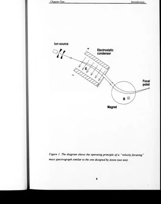
Figure 2. Schematic o f the Wiley-MacLaren lime-of-flight mass spectrometer.
11
P
u
ls
ed
e
xtra
cti
on
v
o
lta
g
[image:36.637.84.590.17.667.2]m _ 1 t
Am 2 At Eq. 1-16
where / is the time-of-flight corresponding to the middle of the peak and At the time-length of the peak at a specified height. The duration o f the ion packet at
the detector results from its initial position spread, and the initial velocity,
energy and spatial spread. It is obvious that the longer the total time-of-flight
and the shorter the time-length o f the packet at the detector, the better is the
resolution.
A method was devised by Wiley and MacLaren [20] to improve the
resolutions of early TOF mass spectrometers to an acceptable level of a few
hundreds. This involved applying suitable pulses to the ion source so as to
compensate partially for the initial spreads of the ion packet. A typical ion
source o f the Wiley-MacLaren instrument (see figure 2) consists of two parts.
The ions are created in the extraction region by a timed electron beam, and are
allowed to drift apart from each other according to their random initial
velocities. The pulsed electron beam has a typical time width of 1 ps. At a
certain time delay (about 1-1.5 ps), a pusher pulse is applied to one of the
sides o f the extraction region. The ions start drifting towards the exit of the
extraction region and ions in the rear of the packet will eventually acquire
more energy than those in the front, therefore they will catch up with them
further down the ion path.
After the extraction region the ions enter the acceleration region where they
Chapter One. Introduction.
utilised to record the arrival times of the ions. The Wiley-MacLaren focusing
was a method to compress a “random” ion packet. This effectively means that
the initial positions of the ions are in no way related to their initial energies
prior to the extraction pulse. Therefore ions at the front of the ion pack can
have higher or lower energies than those at the rear. For this reason Wiley-
MacLaren ion focusing cannot achieve resolutions better than a few hundreds.
The first time-of-flight instruments were only able to analyse low-mass ions,
due to the limitations imposed by the electron impact ionisation. The first
attempt to use TOF for the analysis of high-mass ions was made by Dole et al
in the late 60’s [21,22], The ionisation method used was electrospray and the
sample was polystyrene.
The next step in time-of—flight mass spectrometry came when Macfarlane
showed that high-mass molecules could be ionised efficiently by the fission
fragments from radioactive 252C f [23,24]. A schematic o f the plasma
desorption mass spectrometer is shown in figure 3. The extraordinary
characteristic of the plasma desorption instrument is the short time-length of
the ionisation process (<lns). This time is much shorter than the production
times caused by any other ionisation method. Additionally, every cycle of the
instrument is triggered by detecting fragments of the same fission event that
created the analyte ions, therefore timing circuit jitter can be minimised.
Resolution in plasma desorption linear time-of-flight instruments can be in
excess of 1000-2000, limited by energy spread of the resulting ion beam.
Fisión fragment detector
Acceleration grid
f~Q Molecular ions
* 0 Fragment ions
Ion detector Sample foil
[image:39.641.17.593.13.658.2]Chapter One. Introduction.
1.1.2.3 Ion reflectron in time-of-flight mass spectrometry
In 1966 Mamyrin et al [25] proposed a way to correct the time spread which is
due to the initial velocity spread o f the ions, with the use o f a decelerating and
reflecting field. The idea was that for ions of the same m/q ratio (where q is the number of electron charges of the ion) entering such a field, those with higher
energies will penetrate deeper into the field than those with lower energies.
Therefore the former will spend more time into the reflecting field and they
will “catch up” with the lower energy ions further down the flight path.
In the ideal case above, the time-width of the peaks of the mass spectrum will
only depend on the time-width o f ion formation. In practical cases, there are a
number of time-widening parameters, including the spread in positions o f ion
formation, initial velocity spread, ion optical aberrations, metastable formation
as well as technical/technological problems (electronic stability, time
resolution o f detection system). All of these degrade resolution to a certain
extent.
1.1.2.3.1.1 Single stage reflectrons.
Single-stage reflectrons are the simplest form of ion reflectrons. The reflecting
electrostatic field simulated by a single-stage ion mirror is a simple
homogeneous field created by two flat grids. The first grid is at the entrance of
the mirror and the second at its end. The latter can be replaced with a solid
electrode, although usually a grid is used to allow ions to reach a detector
behind the mirror for linear time-of-flight experiments when the ion reflector
is grounded. In order to improve the homogeneity of the field, a number of
equally-spaced ring electrodes are placed between the two end-electrodes,
connected with a chain of equal-value resistors.
A representation of a single-stage ion mirror, as well as a schematic diagram
demonstrating the ion paths in such an instrument is shown in figure 4. The
constant electric field E within the mirror is parallel to the main axis of the instrument, defined as the x axis. It is assumed that E follows a step function where EX=E for jc<0 and Ex=0 for x>0. The ion velocity components perpendicular to the axis remain constant and do not affect the flight time. The
velocity component considered in the following calculations is ox=u0+S,
where u0 is the axial velocity component after acceleration for an ion ejected from the target with zero velocity and 8specifies the velocity spread.
The incident angle of the ion beam to the field region being 8\ the following relationship is obtained:
mUg /2 = qeV0 cos2 8= Ek
The flight time of an ion with zero initial velocity is calculated first. It is
convenient to define a reference plane perpendicular to the x axis just out of the acceleration region, as shown on figure 4, and to calculate the time-of-
flight from this plane to the detector. For the sake of simplicity, corrections
due to the finite distance between the target and this plane will not be
considered here. The distance between the reference plane and the boundary of
Chapter One. Introduction.
Figure 4. Schematic diagram showing the flight path o f an ion in a single-stage reflectron time-of-flight analyser.
detector is Lv Since the axial velocity component is simply reversed by reflection, its magnitude is the same in both L t and L2, therefore the time spent in field-free flight is tf(=L/u0 where L=L{+LV The time spent in the mirror is
tM=2uJa, where the acceleration a=qeEtm where qe is the charge and m is the mass. The total time of flight is:
t — t M + tff —2m
qeE Eg. 1-17
When a deviation 8 in the velocity is considered, the above equation becomes
2m / x L t = ~ - (m>+£) +
----qeE ' ’ v0 + 8
Expanding the second term as a function of 8 gives
Eq. 1-18
2m / v L _ L L L
• = — (<4, +^) +----S — + S2— - S } —
qeE u0 u„ u0+ . . . Z
Eq. 1-19 2mv0 L 8 2 mu0 L
J
f 1
f*)
qeE ' u0 _ 1 h>0 qeE v0. - o '
The linear term in this expression is equal to zero when
2mu0 _ L qeE u0
or
E =2m u 2
Chapter One. Introduction.
T0 is the kinetic energy of the ions. For this value of E, lM=l,(=L/u0, i.e. the ion spends the same amount of time in the mirror and in the field-free region. The
flight time is:
It is therefore independent of axial velocity to the first order for ions of every
mass. To the first approximation the time of flight is:
instrument. The stopping distance can be calculated by the expression
Ta=lqeE=l4TJL. so /=£/4. As the average axial velocity inside the ion mirror is
vJ2, the effective length is twice 2 x L/4=L.
1.1.2.3.1.2 Double stage reflectrons.
From the preceding section it is obvious that using a single stage ion reflectron
as part of a time-of-flight instrument results in velocity spread correction to
the first approximation. As Mamyrin has shown [25,26,27], it is possible to
make the second order term vanish as well by introducing another free
parameter in the equations of motion. This is achieved by using a double stage
mirror. There is a second grid within the ion reflectron, in order to define two
homogeneous field regions with different electrostatic field values. In figure 5
the schematic of a double stage reflectron is shown. Mamyrin introduced a
Eg. 1-21
Eg. 1-22
The flight time is proportional to yjm/ge , as in a linear time-of-flight
way to represent the energy spread of the ions: the ion energy after the ion
source is U=KU0, where U0 corresponds to the mean energy of the ions
(=qeU0). For low relative energy spreads, K is close to unity and can be represented as K=\+e where £ « 1 .
The total time of flight in this instrument from the exit of the ion source to the
ion detector is t = t L +1B + t R where tL is the total time of flight in the field free region, tB and tR are the flight times in the retarding and reflecting regions respectively. The following relationship applies:
where dB, UB, dR and UR are parameters of the ion mirror regions (length and potential, Figure 5). The above equation can be reduced to
Eq. 1-23
Eq. 1-24 L
Chapter One. Introduction.
+ U .
Figure 5. Schematic o f a time-of-flight mass spectrometer with a double stage ion reflectron.
where F, is a function representing the dependence of t on K=U/U0 with parameters
4d„U0
L U B ' Ar
M rUq
LU R ’ P =U0
It can be seen from Eq. 1-23 that the flight time t is a function of 4 parameters
1jl.Ujl.Ujl
L ’ U0 ’ U0
and K, which is a representation of the range of the permitted ion energies
UmJ U min. In figure 6 a multiple graph is shown representing the above function for different values of the free parameters. Case (a) represents the
optimum situation, where times-of-flight are equal at points 1 and 2 as well as
3 and 4 and d//dt/= 0 at points 2 and 3. Hence there are four coupled equations
(one for each o f the four points) whose solution for the given value
enables the whole set of parameters to be determined. The resolution for the
optimum case is
R = = *« " A U 2(/m„ - / mln)
Schmikk and Dubenskij [28] first published such considerations. A more
recent paper with a similar approach [29] reported that for UmJ U mln = 1.05, 1.1 and 1.2 the ultimate resolution becomes 370 x 10\ 50 x 103 and 7 x 10³
Chapter One. Introduction.
Figure 6. Ion flight times as a function o f energy in a time-of-flight mass analyser with a double-stage reflectron [30],
1.1.2.3.1.3 Quadratic field reflectrons.
The addition of a second finite region of different potential gradient can make
the second-order time aberration term vanish, resulting in large resolution
enhancement for ion beams with higher energy spreads. Extending this
reasoning further, if a field with an infinite number o f appropriate changes of
potential gradient was introduced, all orders of time aberrations could be made
to vanish. Such a case would mean that the flight time in the ion reflectron
would be completely independent of the initial velocity of the ions and would
only depend on the mass over charge ratio. The physical analogue o f a mirror
with this characteristic is a pendulum, where the frequency of a body is only
dependent on its mass and the length of the pendulum. The potential
distribution equation that describes such an electrostatic field has the general
form (figure 7):
k, a and C are constants, a is the coordinate of the point of potential minimum. The equation o f motion along x is:
q is the number of charges of an ion. Adopting qe/m > 0 and k > 0, solution of the above equation is readily obtained:
Eq. 1-25
x = - — k - (x - a)
m Eq. 1-26
Chapter One. Introduction.
Figure 7. Potential distribution in quadratic fields along the ion optical axis x is the initial coordinate (starting point) o f an ion. 2a-x0 is the coordinate o f ideal time focusing.
The frequency of oscillations co is given by:
CO
- ( * )
Eq. 1-28x0 is the initial coordinate of an ion and V0 is the accelerating potential experienced by the ion.
From Eq 1-27 it is obvious that after integer numbers of half-periods:
T„ = ( —) ■" n=l,2,3... Eq. 1-29
That is to say that, after each reflection in the field coordinate x becomes:
x(T„) = a + (x0 - a ) - (-1)” Eq. 1-30
Thus reflection is completely independent of the initial energy qeV0.
The Laplace equation must be satisfied for any electrostatic field. As shown in
[31], Eq. 1-25 becomes on applying this condition:
U( x , y , z ) = j • (x - a)2 + W(y,z) Eq. 1-31
where
<?W & W
cÿ2 + â 2 - k Eq. 1-32
Considering an ion beam with initial parameters ion energy spread qe,
coordinate spread A and angular spread in all directions a reflected in a three-
dimensional field as described above, flight time T„ remains independent of all
Chapter One. Introduction.
M » * - 4-«....f M
? )
Eq. 1-33The above equation is equivalent to TOF focusing up to infinite order
(including first-order, second-order, third-order etc.) for any set o f the initial
parameters, therefore the term "ideal time-focusing" seems to be the most
appropriate.
As shown in [32], the variety of fields with ideal time-focusing is much wider
than those described by Eq. 1-31, 1-32 above and includes a number of static
electromagnetic fields. When demands o f high transmission and especially
simplicity of construction are taken into account, however, it appears that only
a few fields can be practically useful, all o f them being electrostatic. These are:
1) axially-symmetrical hyperbolic potential:
U(r, z) = ^ - ( z - o ) ! - j - r ! + C Eq. 1-34
r, z are cylindrical coordinates, k, a and C are constants.
2) planar hyperbolic potential [33, 34]:
Eq. 1-35 a, b and d are constants (usually b=d=Q).
3) axially-symmetrical hyper-logarithmic potential:
Eq. 1-36
d>0 and b>0 are constants [35].
Chapter One. Introduaion.
The main drawback of fields described above is their high divergence in the r
-or ^-direction. F-or example, the equation of motion along y in the field
described by Eq. 1-35 for b=0 is:
where y0 is the initial y-coordinate and tana is the tangent of the initial angle to they-axis. The hyperbolic functions in Eq. 1-38 means that the motion along y
is unstable and a detector of large size is necessary. For ions starting from a
narrow slit (i.e. when y0 may be neglected) and reflected once in the quadratic
field, it may be shown that the detector dimension in the y-direction should be
sinh(n)/7t~ 3.676 times larger than that in z-direction.
An account of theoretical considerations on quadratic fields was presented by
Rockwood and [36] Yoshida [37] demonstrated the construction o f a tim e-of-
flight instrument featuring an ion mirror with a rotationally symmetric
quadratic electrostatic field (figure 8). The field was sustained by a number of
ring electrodes connected with a resistor chain. The resistors were
appropriately chosen so that each electrode has the correct potential to
approximate the chosen field function in the centre axis of the mirror.
A way of creating a rotationally symmetric quadratic field, without utilising
flat finite electrodes, is to use a pair o f cylindrical symmetry appropriately
Eq. 1-37
or
Eq. 1-38
shaped electrodes: one conical and one hyperbolic electrode arranged as
shown in figure 9. A time-of-flight instrument with a pair of pure
mathematical geometry large-scale electrodes is under construction in the
department of Chemistry, University of Warwick. A laser ion source situated
near the apex of the cone creates an ion packet that time-focuses at the
theoretically optimum position for the mirror geometry.
Cotter and coworkers have described a reflectron time-of-flight mass
spectrometer, where the potential distribution in the ion mirror empirically
approximates that o f a rotationally symmetric ideal ion reflectron [38]. The
main difference between this instrument and that of Yoshida is the longer
field-free region in the former.
Hamilton and coworkers have [39] described a pure-geometry prototype
instrument featuring the planar symmetry quadratic field described by Eq, 1-
35. It comprised a 90° vee electrode kept at ground potential and a hyperbolic
surface at a high positive potential F„ (see figure 10). If the trajectory of an ion
remains on the bisector of the vee, the ions time of flight from x=0 back to x=0
is given by
the square root of the ion’s mass to charge ratio and is independent from its
energy.
This instrument was designed for in-space elemental analysis of ions in the
solar wind. It was therefore compact in dimensions featuring very short flight
times ( up to 392 ns for Fe ), making the achievement of high resolution
problematic. Nevertheless, its ideal focusing characteristics allowed resolution
in excess of 100 for high energy-spread beams.
1.1.3 Ionisation techniques.
1.1.3.1 Historical overview
Evolution o f mass spectrometry has been as dependent on discovery of new
ionisation techniques, which opened new horizons in new compounds to be
studied and methods to be standardized, as on development of novel analysers.
Discharge ionisation may have been what sparked the interest in the
unexpected parabolic shapes in Thomson’s first mass spectrometer, but broad
acceptance of the technique came when electron beam ionisation (El) was
proven to ionise consistently gaseous atoms and small molecules. The next
important step was field ionisation [40,41], chemical ionisation [42,43], and
especially with the discovery o f lasers, photo-ionisation [44,45].
The main limitation of all the above techniques was that they could only ionise
volatile, and therefore relatively small compounds that could be readily
transferred to the gas phase; no existing method could work with non-volatile
Chapter One.
Introduction.
spectrometry after the discovery of El was the introduction o f various
desorption/ionisation techniques that allowed large, non-volatile molecules to
be brought to the gas phase, ionised and analysed in a mass spectrometer. The
most important o f these techniques are field desorption (FD) [46,47],
thermospray ionisation (TI) [48], secondary ion mass spectrometry (SIMS)
[49,50], fast atom bombardment (FAB) [51,52,53,54], plasma desorption (PD)
[55,56], electrospray ionisation (ESI) [57,58], and laser desorption (LD)
[59,60], of which matrix-assisted laser desorption/ionisation (MALDI) [61] is
the most important branch. The most important desorption/ionisation methods
are reviewed here.
1.1.3.2 Liquid - secondary ions mass spectrometry (L-SIMS).
Although initially SIMS was performed using dry samples, it was discovered
that the use of a liquid matrix greatly enhanced stability, sensitivity and
reproducibility of the technique. Hence fast atom bombardment (FAB) as well
as liquid-SIMS (L-SIMS), techniques that evolved from SIMS, utilised liquid
matrices. Most L-SIMS ion sources use Cs as bombarding ions. The Cs are
typically accelerated to potentials in the order of 10 keV or higher (figure 11)
and focused on the sample-droplet. The sample is a mixture o f the analyte
with a liquid matrix, such as glycerol. L-SIMS is routinely used for high-mass
biological macro-molecules, up to approximately 10 000 Da in molecular
mass [62]. It is a “soft” ionisation technique, inducing little fragmentation of
the fragile biomolecules. It is an essentially continuous ionisation method,
Chapter One. Introduction.
Sample probe
Figure 11. Schematic diagram o f an L-SIMS ion source.