University of Warwick institutional repository: http://go.warwick.ac.uk/wrap
This paper is made available online in accordance with publisher policies. Please scroll down to view the document itself. Please refer to the repository record for this item and our policy information available from the repository home page for further information.
To see the final version of this paper please visit the publisher’s website. Access to the published version may require a subscription.
Author(s): David Ronayne
Article Title: Which Impulse Response Function? Year of publication: 2011
Link to published article:
http://www2.warwick.ac.uk/fac/soc/economics/research/workingpapers/ 2011/twerp_971.pdf
Which Impulse Response Function?
David Ronayne
No 971
WARWICK ECONOMIC RESEARCH PAPERS
* The dataset used, along with the original programming can be obtained by visiting http://www2.warwick.ac.uk/fac/soc/economics/staff/phd_students/dronayne. All the programming and ideas presented in this paper are my own unless otherwise stated. I would like to thank Prof. Jeremy Smith for his help and support. Thanks also to Prof. Òscar Jordà, a former PhD student of his Yanping Chong, the members of the online community Statalist and Stata Technical Help for their helpful correspondences. Any mistakes or inaccuracies are my own.
Which Impulse Response Function?
David Ronayne*
University of Warwick
10 October 2011
Abstract
This paper compares standard and local projection techniques in the production of impulse
response functions both theoretically and empirically. Through careful selection of a
structural decomposition, the comparison continues to an application of US data to the
textbook ISLM model. It is argued that local projection techniques offer a remedy to the bias of the conventional method especially at horizons longer than the vector autoregression‘s lag
length. The application highlights that the techniques can have different answers to important
1) Introduction
Econometric application of macroeconomic models is one of the most important aspects
within quantitative economic analysis. This paper works to explain what it believes to be the
most significant and cutting-edge contributions in the field, combining them in an application
of US data to the textbook ISLM model.
Ever since the Cowles Commission was established in 1932, the development of related
empirical techniques has drawn an increasing amount of attention. Perhaps the most
important contribution was Sims (1980) and the inception of vector autoregressions (VARs).
The VAR methodology offered a powerful new analytical weapon – the impulse response
function (IRF). IRFs are used to track the responses of a system‘s variables to impulses of the system‘s shocks. Sims‘ paper spawned a wealth of literature applying the technique. However
it was not long before a pertinent objection was made to the procedure. Orthogonalising the VAR‘s shocks is required so that the shocks tracked by IRFs are uncorrelated. Authors such
as Cooley and LeRoy (1985) and Pagan (1987) pointed out that the original recursive
structure of Sims to do this imposed arbitrary and potentially harmful restrictions on the
system. To impose restrictions on which variables affect which others is a powerful statement
about the underlying structure of the system, and will affect empirical output including IRFs
and forecast error variance decompositions (FEVDs). Combining the needs of identification
and non-arbitrary orthogonalisation has since become the focus of structural VAR (SVAR)
analysis.
Implementation of SVARs is far from uniform and there exists a vast literature debating how
it should be done. Deliberation over this in order to select one for application constitutes the
first component of this paper. The second component concerns the method of IRF production.
from Jordà (2005) aims to remedy some of these problems. Owing to its youth, how well this
method competes in theory and practice is relatively unknown. This paper discusses the
existing research and adds some of its own insights. Using software not previously used to
carry out the procedure; an application of the ISLM model based on Keating (1992) is
conducted. The application serves as the culmination of the two components of the paper,
demonstrating both the ability of the ISLM model to describe the data and the implications of
the IRF technique employed.
Section 2 discusses the literature on competing SVAR methods; Section 3 qualitatively compares Jordà‘s IRF technique to the standard approach; Section 4 introduces the
application and formalises the notions introduced in the preceding sections; Section 5
provides the results; Section 6 concludes.
2) Structural VAR Identification Schemes
In their review of the VAR methodology twenty years after Sims‘ (1980) original paper,
Stock and Watson (2001) conclude that VARs successfully capture the rich interdependent dynamics of data well, but that ‗their structural implications are only as sound as their
identification schemes‘. This section looks at the attempts which have been considered to
answer the pivotal issue of identification in the literature with an eye to selecting one for this paper‘s own application.
2.1 The Cholesky Decomposition and Short-Run Schemes
Sims (1980) speaks of ‗triangularising‘ the VAR as his method of orthogonalising the
reduced form shocks, and is referred to as a Cholesky decomposition or a Wold causal chain.
This triangularising achieves orthogonalisation but imposes a recursive structure on the
ordered in the VAR will determine which is affected by which in this recursive way.
Cholesky decompositions are easy to implement and simple to understand. Stock and Watson
explain how it was common for practitioners to justify recursive structures so that their
structural scheme coincided with a recursive setup justified by ‗cobbled-together theories‘ that are only ‗superficially plausible‘.1
SVAR studies with more carefully considered schemes quickly became widely used see, e.g.
Blanchard and Watson (1984), Bernanke (1986), Sims (1986), Eichenbaum and Evans (1995),
Sims and Zha (2006), Basher et al. (2010). Non-arbitrary orthogonalisation schemes which
impose contemporaneous restrictions on the VAR are referred to as short-run identification
schemes. Most short-run restrictions are zero restrictions e.g. that output reacts only with a
lag to monetary shocks. Although a seemingly reasonable assumption, clearly the frequency of one‘s data is of vital importance; if one had annual data, a contemporaneous zero
restriction is likely to be more debatable than if it were on quarterly or monthly data. It
should be noted that restrictions are not confined to forcing parameters to be zero as in the
Wold causal chain, other linear (e.g. Keating 1992) and non-linear (e.g. Galí 1992)
restrictions are occasionally employed on the contemporaneous relations between variables.
Restrictions can also be implemented depending on assumptions about what information is
available to agents at the time of a shock e.g. Sims (1986), West (1990). Opinions concerning
short-run restrictions are mixed. Faust and Leeper (1997) claim there is often simply an
insufficient number of tenable contemporary restrictions to achieve identification. However,
Christiano et al. (2006) argue that short-run SVARs perform ‗remarkably well‘ by way of the
relatively strong sampling properties of the IRFs they produce.
Short-run models can supply enlightening structural inference in a relatively straight forward
way. However, they are sensitive to the exact scheme employed; justifying one‘s restrictions
based on theory and available data should be a priority. This paper will adopt a short-run
scheme. The relative merits of this choice for the present application are provided by the
following review of other schemes.
2.2 Long-Run Schemes
Pioneering work by Shapiro and Watson (1988) and Blanchard and Quah (1989) described
how restrictions could be placed on the long-run responses (at an infinite horizon) of
variables to shocks e.g. in Blanchard and Quah‘s bivariate VAR of output and unemployment, they identify the shocks as ‗demand‘ and ‗supply‘ shocks by restricting the ‗demand‘ shocks
to have no long-run impact on real GNP.
Bearing in mind the criticisms made against short-run restrictions, restricting long-run
responses was a welcome extension to the tools available for identification. Short-run and
long-run schemes can produce quite distinct sets of results on the same data as shown by e.g.
Keating (1992), McMillin (2001). Lastrapes and Seglin (1995) boast the technique is
advantageous because there is a greater consensus amongst theoretical models in terms of
long-run results. It should be unsurprising therefore that the most common set of restrictions
is to nullify the long-run response of output to monetary shocks. Ever since their introduction,
long-run restrictions have been frequently employed, see e.g. King et al. (1991), Francis and
Ramey (2004), Fisher (2006) among many others. It is also possible to adopt a combination
of short and long run restrictions as originally demonstrated by Galí (1992), and Gerlach and
Smets (1995), Peersman and Smets (2001) and Mamoudou et al. (2009).
Unfortunately, long-run schemes are far from critique-free. Faust and Leeper show that with
exacerbated by long-run restrictions causing serious bias to IRFs even with large samples.
Although the severity of this does depend on the assumptions made about the underlying data
generating process (DGP).
Taylor (2004) shows that under long-run restrictions, a -dimensional model has solutions
for the matrix used to orthogonalise the shocks. Each of these solutions has its own distinct
set of IRFs. This multiplicity of solutions is due to long-run models imposing a set of
non-linear equations which does not result in a unique set of contemporaneous relationships.
There is often no way to choose between the solutions convincingly. One may look at all the
possible sets of IRFs, but this quickly becomes a daunting task, e.g. a 5-variable VAR would
give sets. The multiplicity of solutions is sidestepped with short-run schemes
because they have a unique solution by virtue of imposing the contemporaneous relationships,
so it is known in which direction each variable should be moving immediately after the shock.
Dupor and Kiefer (2008) claim that the term ‗long run structural VAR‘ is basically an
oxymoron. They argue that long run schemes make restrictions on the cumulative response of
a stochastic process so long lead and lag covariances are as important as the short. In practice
however, the number of lags in a VAR is typically short, giving poor estimates of these long
run properties.
2.3 Recent Advances in Identification
Sign restrictions were introduced by Faust (1998), Uhlig (1999), Canova and De Nicoló
(2002). They restrict the response of some variable to some shock to be positive or
non-negative for a number of periods and are especially popular in the technology shock literatre
e.g. Peersman (2005), Peersman and Straub (2009) and Berg (2010). Arguably less restrictive
restrictions have been imposed both to restrict the immediate response of a variable e.g. Faust (1998), and in the ‗medium‘-run e.g. Peersman (2005), or Uhlig (2005) who restricts
variables to respond positively or negatively for six months. Sign restrictions are not only applicable to variables‘ responses. The method of Canova and De Nicoló and application of
Canova and Pina (1999) introduced sign restrictions on the cross-correlations of variables in
response to shocks.
However, the less restrictive nature of sign restrictions is not catch-free. As Fry and Pagan
(2007) show, the common methodology of implementing sign restrictions generates a
multiplicity of models (instead of one). Tools such as FEVDs will give misleading results
because the IRFs generated are not uncorrelated. They suggest a fix and demonstrate the difference it makes using Peersman‘s study as a case in point. They conclude by noting that
to say sign restrictions are a panacea to the problems of previous identification methods is ‗far from the truth‘.
Herwartz and Lütkepohl (2010) suggest a novel way to utilise the information in the VCV
matrices in different regimes for models with Markov switching (MS). A problem is that
attaching structural interpretations to shocks is not possible, so they suggest combinations of
this with the more established schemes described above to create a MS-SVAR model. One
great advantage of this approach is that identification is achieved through restricting regimes‘
VCV matrices to be orthogonal. This means that the validity of any regime-invariant
(conventional) restrictions can be tested. The approach is most promising although not
without its own difficulties, but more application and investigation into the method is
3) Impulse Response Functions
3.1 The Standard Technique
Standard IRF production uses estimates from the estimated VAR model. The usual
methodology for generating IRFs involves non-linear (at horizons greater than one) functions
of the estimated VAR parameters; hereon this method is called VIRF, and the resulting IRFs
called VIRFs. As the horizon increases, so does the order of the polynomial. If the VAR
coincides with the DGP this procedure is optimal for all horizons. If however it does not coincide, it produces biased IRFs. As increases, this bias is compounded by the reliance on
the set of estimated VAR parameters and through the non-linearity of VIRF. However, for , a VAR will produce the optimal one-step ahead forecast. In fact, Stock and Watson
(1999) show that even if the model is misspecified, an AR (and therefore a VAR) process still
produces reliable one-step ahead forecasts outperforming rival, non-linear forecasting
methods.
Non-linearity is not the sole source of bias in VIRFs. VIRFs also typically suffer from large
small-sample biases stemming from bias in the estimated autoregressive coefficients (see
Pope 1990). The small-sample bias in the VIRF‘s confidence intervals is perhaps even more
serious. As Kilian (1998) explains, most intervals for VIRFs are produced from
asymptotically-justified formulae e.g. following Lütkepohl (1990). However, he finds that such intervals are ‗extremely inaccurate‘ in small samples.
Naturally, one wants to approximate the DGP as well as possible. It is commonly expressed that the VAR‘s approximation is inadequate because it is more likely that a set of
macroeconomic variables are better described by a vector autoregressive moving average
(VARMA) process. Palm and Zellner (1974) and Wallis (1977) explain that even where
utilise will in fact be a VARMA process. Cooley and Dwyer (1998) show that real business
cycle models follow VARMA rather than VAR processes. By fitting data with a VAR,
practitioners are likely to be poorly approximating the DGP and by using VIRF methods are
likely to be producing inaccurate IRFs.2
This paper offers an additional benefit of the LPIRF technique here. VARMA processes are
closed with respect to linear-transformations (Lütkepohl 2009) meaning that any linear
function of a finite VARMA process, is itself a finite VARMA process. This is a property
that VAR processes do not have. Most data aggregations for macro variables are temporal
(e.g. generating quarterly GDP from monthly) or contemporaneous (e.g. GDP as the sum of
consumption, investment, government spending and net exports) linear transformations.
Hence, if the underlying DGP is indeed a VARMA process, then any chosen linearly
aggregated data will be too. If the employed technique for producing IRFs performs well for
the VARMA class of models, then one has the added bonus of relaxing about aggregation
issues. Indeed, Lütkepohl (2005) warns that differently-aggregated datasets can produce
drastically different VIRFs, which is another reason to replace confidence with caution when
viewing results from the VIRF technique.
3.2 Local Projection
Jordà (2005) introduced a technique designed to be more robust to misspecification of the
DGP. Instead of using one set of VAR coefficients as in the VIRF technique, he proposes
estimating a new set of estimates for each horizon. This avoids escalation of the
misspecification error through the non-linear calculations of the standard VIRF technique as increases and (the techniques give the same IRFs at ). The technique collects
new estimates for each forecast horizon by regressing the dependent variable vector at
on the information set at time . In other words, the projections of forward values of the
dependent variable vector on the information set are local to each horizon. IRFs produced
using this technique (hereon LPIRFs, and the technique LPIRF) are easily produced as they
are simply a subset of the estimated slope coefficients of the projections.
Furthermore, as LPIRFs do not involve the same non-linearities as VIRFs, they are more
likely to be well-approximated by Gaussian distributions and have more accurate confidence intervals. VIRF methods rely on ‗(not always reliable) delta-method approximations and
considerably complex algebraic manipulations‘ (Jordà 2007 p20). The asymptotic
distributions typically used are for the marginal IRF distributions e.g. Hamilton (1994) p336-9. Jordà (2007) gives the joint distribution of the model‘s IRFs. The advantage of this is that
the resulting distribution represents that IRFs are serially correlated and is able to answer
questions about the collective shape of IRFs, rather than individual point IRF estimates –
which is what a string of marginal confidence intervals would do.
Jordà (2005) provides Monte Carlo evidence which shows that LPIRFs are more robust to
lag-length misspecification, are consistent, and are only ‗mildly‘ inefficient compared to IRFs
of the true DGP he uses. Other benefits of the technique are that they are easy to implement
practically (simple univariate regressions suffice), and that it can be easily adapted to
non-linear specifications (a cubic specification is common). LPIRFs have been well-used since.
Hall et al. (2007) produce LPIRFs in a DSGE context, Haug and Smith (2007) conduct a
comparative study of structural VIRFs and LPIRFs and Ho (2008) investigates the
relationship of exchange rates and monetary fundamentals.3
However, the LPIRF approach has received criticism. The LPIRF and VIRF techniques are
asymptotically equivalent if the DGP is stationary and linear e.g. a stationary VAR. A natural
question is how well these methods compare in small samples. Kilian and Kim (2009) use an empirical exercise to show that the LPIRF‘s bias is greater than the VIRF‘s when the
underlying DGP is a VAR process. Relatedly, they also find that the LPIRF asymptotic
intervals are much wider than VAR-based estimators, and by virtue of that are more accurate.
As the sample size increases (in their study from 100 to 200) the VIRF confidence interval
estimator has similar accuracy as the asymptotic LPIRF interval estimator, although again the LPIRF‘s intervals are wider. The VIRF interval production referred to by Kilian and Kim is
the small-sample bias correcting bootstrap method of Kilian (1998). It must be said that the LPIRF‘s intervals generally outperformed other VIRF interval estimators. Resting on the
results of this ―best‖ VIRF interval estimator, and the usual VIRF point estimates, they
conclude that there is no reason to abandon the VIRF method.
That the bias of the VIRF lower is hardly surprising as the VIRF method is optimal when the
underlying process is a VAR. What is more worrying is that they obtain similar results when
the DGP is assumed to be a VARMA(p,q) process i.e. an infinite-order VAR process.
Although for larger values of q (the MA order), and hence the poorer estimate a VAR is, the
accuracy of the VIRF estimator and the asymptotic LPIRF estimator is similar. One would
naturally conjecture that there would be a point where the DGP is far enough from a VAR for
the LPIRF to become more attractive than the VIRF. Indeed, Kilian and Kim call for such an
investigation, referring to their work on the VAR only approximating the DGP as ‗preliminary‘.
Although Kilian and Kim‘s evidence is persuasive, this paper offers some points in defence
of LPIRFs. Jordà‘s (2005) Monte Carlo evidence showed was that the method is more robust
to lag length misspecification. As Braun and Mittnik (2002) show, the same is far from true
of the VIRF technique. They find that misspecification of lag-length causes a large
on the VAR‘s ability to approximate a likely VARMA DGP, Kilian and Kim did not use a
specification that showed LPIRF to be strictly superior, although it was argued it seems likely
that one could. Adding more lags to a VAR will naturally improve its fit to an underlying VARMA (or VAR(∞)) process. But because adding a lag to a -variate system adds
regressors, if many lags need to be added to make the VAR‘s approximation good in a
multivariate model, the number of degrees of freedom is quickly reduced, and the required
sample size quickly becomes unwieldy.
Depending on the context, either VIRF or LPIRF methods could be argued superior. The
properties of the VIRFs are much better documented owing to their longer history. However,
there have been some substantial efforts into formalising and discussing its asymptotic and
theoretical attributes, strengths and weaknesses.
Due to the uncertainty in the underlying DGP of the macroeconomy and the similar
performance of the LPIRF and VIRF estimators in non-small samples (approaching 200
observations), the proceeding analysis estimates IRFs through both methods, facilitating
comparison. The joint asymptotic confidence intervals for the LPIRFs of Jordà (2007) are
applied due to the larger sample size and because they have been shown to be more accurate than the LPIRF‘s bootstrap method.4
4) Methodology
This section formalises the techniques discussed in the previous sections and provides the
methodology used to produce the results of this paper which are presented and discussed in
section 5.
4.1 Structural Identification
4.1.1 Theory
Consider a structural vector autoregressive model, written as:5
( ) (1)
where is a vector of variables of dimension at time t, ( ) is the pth order matrix
polynomial in the lag operator , is the matrix of coefficients determining the
contemporaneous relationships, and ( ) is the vector of structural shocks. The
reduced form (RF) estimable with data is:
( ) (2)
where ( ) is the vector of reduced form residuals. The latter is more readily
interpretable and is focussed on for identification.6 As can be seen in (1), the structural form
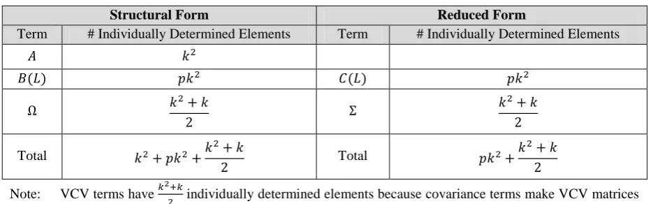
(SF) has more parameters than the RF in (2). Table 1 counts the number of parameters in
[image:15.595.65.533.524.670.2]each form.
Table 1 – Number of Parameters of Structural and Reduced Forms
Structural Form Reduced Form
Term # Individually Determined Elements Term # Individually Determined Elements
( ) ( )
Total Total
Note: VCV terms have individually determined elements because covariance terms make VCV matrices
symmetric.
5 In the language of Lütkepohl (2005) this is an ‗A‘ model, where focus is solely on the matrix A in (1) in the link between reduced and structural forms. Often ‗B‘ or ‗AB‘ models are used which would specify ( ) and identifying restrictions would be placed on A and B. One can think of A and B models as
Comparing the totals, unique identification of the SF parameters requires restrictions.7 A
standard assumption about the structural shock vector ( ) is employed, i.e. that the
structural VCV matrix is the identity. This makes ( ) distinct restrictions. Restricting
implies that structural shocks come from distinct sources as is diagonal, and that
each of the structural variances is unity as has a unit diagonal. It can be of interest to allow
to have estimable diagonal elements, but this paper‘s employed software requires this
assumption.
The final ( ) restrictions are placed on the matrix and are the more contentious
restrictions which the discussion of section 2 focused on. As the elements of determine the
contemporaneous relations between the variables, restricting them will dictate the shape of
the IRFs and must be theoretically justified.
4.1.2 ISLM Application
This paper utilises the structural identification scheme of Keating (1992). The dataset used
comprises of quarterly US data for prices (CPI all items), interest rates (3-month rate), money (M1) and output (real GDP) ( and ) from 1964:3 to 2009:3.8 Keating‘s restrictions
appeal to the theory of the standard IS-LM model so that the resulting structural disturbances may be identified as: ―aggregate supply‖, ―money supply‖, ―money demand ‖ and
―investment and savings‖ or AS, MS, MD and IS shocks. The 4-variate system requires
( ) identifying restrictions on in order to just-identify all 4 shocks. The
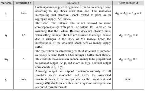
rationale for these is detailed in Table 2 below.
7 More generally, the ‗AB‘ model requires restrictions, but in the ‗A‘ or ‗B‘ model restrictions are made implicitly through setting either A or B to be .
Table 2 – Rationale of Restrictions
Variable Restriction # Rationale Restriction on
1,2,3
Contemporaneous price exogeneity: firms do not change price according to any shock other than one. This motivates interpreting that structural shock related to price as an aggregate supply (AS) shock.
4,5
The short term interest rate is not allowed to move contemporaneously with prices or output; this is based on assuming that the Federal Reserve does not observe these when setting the rate. The Fed are assumed to change the rate due to changes in the stock of M1 money, hence the interpretation of the structural shock here as money supply (MS).
6
The motivation for interpreting the third structural disturbance as money demand (MD or LM) through a buffer stock theory. This restricts movements in nominal money to be proportional to nominal output. As and are in logs, nominal output corresponds to .
none
Allowing output to respond contemporaneously to all variables seems reasonable and leaves the associated structural shock to be interpretable as the investment and savings (IS) shock. Indeed this fourth equation corresponds to a reduced form IS formula.
none
For clarity, (3) shows how the restrictions are placed on the impact matrix:
( ) ( ) ( ) (3)
As (3) shows, the chosen IS-LM identifying restrictions cannot be imposed by a Cholesky decomposition, requiring estimation of ‘s free parameters via full-information maximum
likelihood.9 However, it will be useful for later to note that a Cholesky decomposition will
allow interpretation of the AS and IS shocks in the same way, but lose the structural interpretation of the second and third equations‘ shocks. To see this consider the implications
of a lower triangular matrix, noting the similarities and differences with (3):
(
)
( ) (
)
4.2 Impulse Response Functions
4.2.1 Definition
The concept of an IRF is formalised in (4):
( ) [ | { ( ) ] [ | ( ) ]
That is to say IRFs measure the reaction of the system‘s variables at , for to
a shock of the disturbance vector of . is the information available at which is the set of
lagged dependent variable vectors up to lag order . In this 4-dimensional structural analysis,
the shocks , which correspond respectively to shocks. The
structural shock corresponds to the column of ̂ where each row corresponds to the
response e.g. ̂ would be the response of to an shock at the time of the shock.
Hence the matrix is the ―impact matrix‖ that holds the information on ( ) for .
Attention now turns to the two distinct methods of producing IRFs discussed in section 3.
4.2.2 VIRF Theory
VAR-based impulse response functions are found by noting that any VAR( ) model e.g. (2)
has a VMA( ) representation:10
̅ ( )
10 I referred to Enders (2001) and Hamilton (1994) when needed.
( ) ( )
Note that we can split this into pre-shock, shock and post-shock components:
̅ ∑
∑
Using this with the definition of an IRF in (4) and structural impulse vector :
( ) [ ̅ ∑
] [ ̅ ∑
]
( ) (5)
Where (5) is the ( ) response vector of the systems variables at time to the
structural shock of time . It may more clearly show the structural link to give the impulse
response matrix by recalling that the are the columns of :
( ) (6)
Which reinforces why is referred to as the impact matrix:
( )
To see how to derive the VIRFs from the estimated reduced form VAR for explicitly,
one should note the implied recursive relationship between the MA and AR ( ( )) operators
because ( ) ( ) or rather that ( ) ( ) , implying unique coefficients on the
lag operator terms. Hence the IRFs are generated recursively:11
∑
∑
Finally, to generate the structural impulse responses as in (6), the above set of derived MA coefficients (7) need to be post-multiplied by – as it stands the impulse was not structural
but the shock comprises of a unit innovation to the equation as shown by .
By the above derivations one can appreciate the non-linearity that was accused to be a source of the VIRF technique‘s bias. Expanding the expressions to state them in terms of the AR
coefficients only:12
( )
( )
There are two relevant points of interest from (9). The MA coefficients are polynomials of
the AR coefficients, is a highly non-linear function.13 The order of the polynomial is
12 Derivations are given in TA.1.
(7)
increasing one-for-one with the horizon. The number of, and complexity of the interaction
terms following the lead term are also increasing. These highly non-linear polynomials show
how any bias in the AR estimates will be magnified as the horizon increases.
As has been noted, VIRF produces optimal one-step ahead forecasts. The crux of the reason
for this result can now be fully appreciated. As shown by (8) VIRF uses the AR(1) coefficient
matrix estimate from a regression of the dependent variable vector one-step ahead of the first
regressor. In other words, the VAR regression estimates coefficients local to the one-step
ahead horizon, and thus suffers less from any misspecification of the underlying DGP. The same is not true at horizons due to their reliance on the same set of coefficients local to
.
4.2.3 LPIRF Theory
Impulse response functions generated by local projection aims to eliminate the cause of the
bias in the VIRF technique by estimating (projecting) locally to each forecast horizon, not just . To conduct LPIRF one needs to run a collection of ―forwarded projections‖ on
the information set. By Jordà‘s (2005) original notation:14
(10)
The timing convention (denoting the coefficients as corresponding to the horizon) may
seem a little strange here. To explain, consider the first projection at , which reduces
(10) to a VAR. When using VARs to produce IRFs as in section 4.2.2 it was shown that
13
The exact form of (other than its non-linearity and increasing non-linearity with ) is not necessary for the present discussion and points made. If interested, the reader is directed to TA.1 for a closer inspection of the recursive formula‘s expansion.
( ) , the first AR coefficient multiplied by the shock. Hence the
same is true of the VAR here ( in the language of (10) will give the first-horizon IRF)
i.e. ( ) . LPIRFs depart from VIRFs at ( ). To derive the LPIRF
it is simpler to adopt the clearer notation for the projections, adapted slightly from Kilian and
Kim (2009):15
(11)
Using (11) and the definition of IRFs (4) the LPIRFs are derived as such:
( ) (12)
The LPIRFs of (12) are simply the first matrix of slope coefficients of the local projections. For , (11) is a VAR and ( ) , hence the LPIRF technique does not
stray from the optimal one-step ahead forecast estimator.
On a practical note, the nature of LPIRF generation means that one cannot forecast further than the sample size, and the sample size available for each projection falls one-for-one as
(or ) increases. VIRF only loses observations as increases.
The main arguments in the literature have been summarised in section 3, but can now be
appreciated. The key difference between the procedures is that LPIRF directly utilises single
coefficient matrices (12) instead of VIRF which relies on non-linear transformations (9). By
producing coefficients local to each horizon, deviations of the DGP from the VAR in (2) will
15 Giving Jordà‘s admittedly less clear expression is included because the technique is relatively new and is not standard in text books, so the original form is a good reference point.
𝐿𝑃𝐼𝑅𝐹(𝑡 𝑑𝑖) 𝐸[𝛼 𝑃 [𝛼 𝑃 𝑦𝑡 𝑃𝑝𝑦𝑡 𝑝 𝑑𝑖] 𝑃𝑝𝑦𝑡 𝑝 ]
not be magnified through a web of non-linearities. This is why Jordà boasts LPIRF is more
robust to misspecification of the unknown DGP.16
5) Estimation and Results
This section deals with the standard issues involved in VAR analysis then presents and
discusses the results. An original contribution of this paper is that it offers an application of
the LPIRF technique in Stata.17 Jordà (2007 and 2009) offers a slicker way to proceed with
the coding rather than following his original (2005) paper, which this paper adopts.18 A
second original contribution of this study is that it combines structural identification with
both the LPIRF and VIRF techniques. Although this has been done e.g. see Haug and Smith
(2007), there are very few examples, and this is the first explicit ISLM application.
5.1 Data Issues
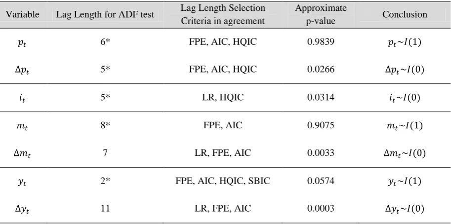
Generating results with appropriate standard errors requires the variables to be stationary.
Under the assumption that our series are difference stationary, a series of unit root tests are reported in Figure A.1 in the appendix to ascertain the order of integration of and
.19 The results suggest that the vector ( ) is stationary.
Lag length selection criteria shown in Table A.2 initially suggest inclusion of 7 lags in the
VAR (following the AIC and final prediction error). The Schwarz‘s Bayesian (SB) and
Hannan-Quin information criteria do suggest fewer lags due to the way they penalise the
16 Focus has been on the point estimates of the IRFs. VCV estimates are of course vital for inference but have not been explicitly derived and focused on beyond the qualitative discussion of section 3. This is both because the point estimate comparison highlights the main advantage and rationale for LPIRFs and because of limited space. However, TA.2 ii gives the formulae used for the asymptotic LPIRF VCV estimates.
17 Applications typically involve Gauss or Matlab, I was not able to find one in Stata. It is my hope that this effort can help to popularise the use of the LPIRF technique by using Stata. The current code is not available as a Stata download command as it is written specifically for my application. The file I used is available to download at http://www2.warwick.ac.uk/fac/soc/economics/staff/phd_students/dronayne it is not the most elegant or efficient, but I hope it will help anyone else interested in creating their own version.
18 The procedure for estimation does not add sufficient intuition to warrant inclusion in the main text, hence the skeleton of the procedure used is provided in TA.2.
inclusion of extra lags. Although the SBIC is consistent, the AIC is often used as authors err
on the side of caution wanting to avoid misspecification, albeit at the cost of inefficiency. The
LM test shown in Table A.3 shows the presence of serial correlation at orders 1, 5 and 8 at
the 10% level. Specifying 8 lags removes all rejections of the null (no serial correlation) at
the 10% level. The price of one extra lag – 16 extra slope parameters for the VAR estimation
and one fewer observation for the generating the LPIRFs – is not trivial, but to avoid the
possibility of misspecification with a healthy sample size of 172, seems a worthwhile trade off. No time trend is included as it is insignificant in all the VAR equations except where
it was very small (-0.00003), and trend inclusion has a negligible impact on results.
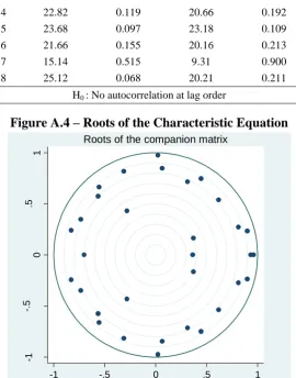
The stability condition for VAR estimation requires that the roots of the related characteristic
equation lie within the unit circle (solutions can be real or imaginary). If satisfied, the variables will be jointly covariance stationary, or ‗non-explosive‘. In the present 4-variate
8-lag model there are 32 roots to check, all of which lie within the unit circle as Figure A.4
shows.
5.2 Impulse Response Functions
Before turning to the IRFs, a few points require attention. The Cholesky scheme is an important and required component of the analysis. Jordà‘s asymptotic VCV derivations for
short (and long) run schemes are valid for on recursive schemes only. Given the downsides
expressed for recursive schemes in section 2 this is a nuisance, but confidence intervals are
important for meaningful analysis if one can properly identify shocks. Although the
Cholesky decomposition still allows the AS and IS shocks to be identified (as noted in
section 4.1.2), this paper uses the scheme to compare the IRF techniques rather than to make
structural conclusions. There is nothing preventing LPIRFs to be produced without
these is of course hindered by the absence of standard errors, but they will allow statistically
tentative but fully structural insight.
The longest horizon is chosen to be . As these data are quarterly, this provides a
6-year horizon, a decent medium-long span. VIRFs can be estimated for any (although with
increasing bias and diverging confidence intervals) but LPIRFs are limited (as discussed in 4.2.3). With a sample size of 180 and a VAR(8), is selected so that each projection
has observations.
5.2.1 Structure-Free Observations
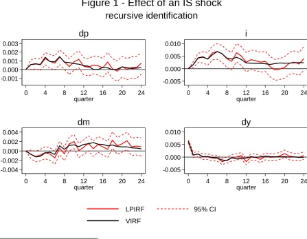
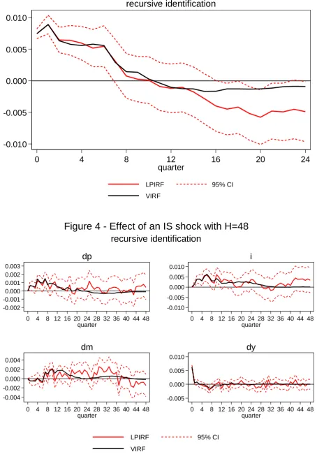
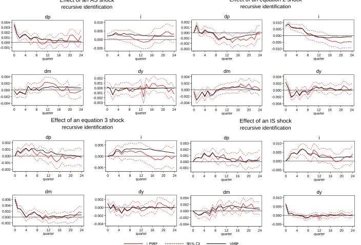
Figure 1 displays IRFs of both techniques along with confidence intervals for the LPIRFs
from an IS shock using the recursive decomposition.20
20 In the graphs, d stands for delta to signify that the variable is in first differences. The full set of IRFs for the recursive scheme is given in Figure A.6.
-0.001 0.000 0.001 0.002 0.003
0 4 8 12 16 20 24
quarter dp -0.005 0.000 0.005 0.010
0 4 8 12 16 20 24
quarter i -0.004 -0.002 0.000 0.002 0.004
0 4 8 12 16 20 24
quarter dm -0.005 0.000 0.005 0.010
0 4 8 12 16 20 24
quarter dy
[image:25.595.73.521.395.742.2]recursive identification
Figure 1 - Effect of an IS shock
The LPIRFs are spiky over all horizons shown. This reflects that LPIRFs at each horizon are
a distinct set of slope parameters. The VIRFs however, are non-linear combinations of the
VAR parameters (9), recursively calculated (see (7)) which effectively smooths the relative
spikiness of a collection of individual parameters. Hence they appear smoother than the
LPIRFs. Further, note that this difference is only pronounced after 8 quarters. This is no
coincidence, the VIRFs are based on a VAR(8) model. Noting the distinction between the equations of (7), VIRFs for [ ] are based on increasingly non-linear functions of
all the estimated VAR coefficients (excluding exogenous terms). As VIRFs receive no new estimates in this range the nature of the formulae dictate they become smoother with .
Within the range [ ] one would still be likely see VIRFs becoming less spiky relative
to LPIRFs due to their recursive nature despite VIRFs utilising a new set of coefficients with each . What is pronounced is the speed at which VIRFs become smoother after the horizon
surpasses the lag length.
VIRFs are indeed typically smooth. While the specific dataset being used is of course influential, this paper suggests that this is typically an attribute for horizons [ ]. If
the DGP is a VARMA process then the LPIRFs are consistent, the VIRFs are biased, but
yield a better fit with longer lag-lengths. This study‘s evidence shows that the VIRFs are seemingly good approximations to the specification-robust LPIRFs for [ ], but that
this similarity quickly becomes worse as increases outside this range. A crude but
illustrative way to demonstrate this is to show the pairwise correlation between the VIRFs
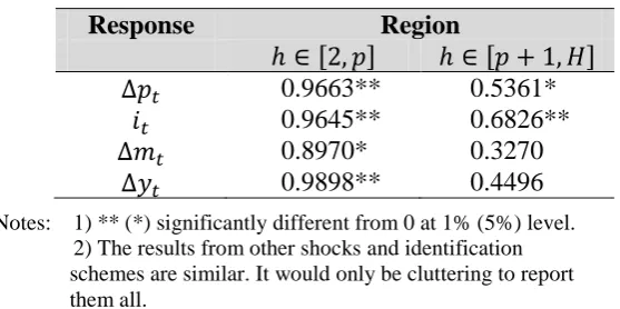
and LPIRFs for both regions (for the IRFs in Figure 1) shown in Figure 2. Simple correlation
is a crude measure because it only picks up linear associations. Nevertheless, it is testament
to the argument developed above. The correlations between the VIRFs and LPIRFs for all
four variables are near 1 (although the association for the change in money is a little lower)
Figure 2 – Pairwise Correlation of VIRF and LPIRF within Different Regions
Response Region
[ ] [ ]
0.9663** 0.5361*
0.9645** 0.6826**
0.8970* 0.3270
0.9898** 0.4496
Notes: 1) ** (*) significantly different from 0 at 1% (5%) level. 2) The results from other shocks and identification schemes are similar. It would only be cluttering to report them all.
As Figure 1 shows visually, the correlation worsens substantially after , which is
reflected in Figure 2. All correlations are substantially lower, half of them insignificantly
different from zero. If VIRFs encompass misspecification bias which increases with forecast horizon which is mitigated by LPIRFs, this analysis suggests the VIRF‘s bias worsens
substantially for horizons greater than the lag-length.
This being said, Figure 1 shows no large practical difference in the prediction of the two
techniques. This is not to be expected in general. Haug and Smith are a case in point. They
compare results from a VAR(1) to LPIRFs. Their VIRFs are so smooth that the majority
appear like a collection of straight lines relative to the spikiness of the LPIRFs (their results
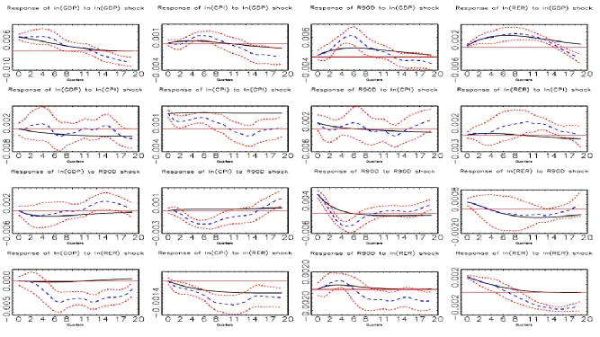
are copied in Figure A.5). Much of the inference from their graphs is very different
depending on the IRF technique chosen. The present analysis using a VAR(8) displays VIRFs
as a better approximation to LPIRFs and thus the results are often qualitatively similar. However, there are some differences in the techniques‘ predictions. Figure 3 shows an
example of a significant difference in the techniques predictions. The shock does not
correspond to any of the structural shocks identified by the scheme of section 4.1.2, hence it is inappropriate to interpret structurally. The IRFs of after 13 quarters diverge, with the
VIRF lying close to the LPIRF‘s upper confidence band ever after, and above it in quarter 20.
significantly less than zero for all horizons (bar ) shown 4 years after the shock‘s
impact.
That the IRFs produce similar predictions with these data is an interesting result. The
aforementioned long lag length of this study allows the VIRFs to be closer to the LPIRFs for longer. As the VAR‘s order is a third of the maximum horizon, this gives the VIRF limited
opportunity to diverge from the LPIRF. Although doubling the maximum horizon to
investigate this still does not result in divergence. Figure 4 shows the same responses as Figure 3 but with .
In fact one could reasonably favour using VIRFs for this application. Firstly, the techniques‘
similarity of output could suggest that they both well represent the DGP and hence that the
DGP is well approximated by a VAR process or by a VARMA process with relatively short
MA component. In situations where the DGP is a VAR process, Jordà (2005) notes that VIRF
is more efficient and Kilian and Kim (2009) argue that LPIRF intervals will be less accurate
than the appropriate VIRF intervals. In situations where the DGP is a VARMA process, it
was suggested there may well be a point where LPIRFs are more accurate than VIRFs. There
is no definitive method to choose between them, and when they produce similar output as in
the present application, the right choice is not obvious. Secondly, one may simply argue that the VIRFs are smoother (especially at ) and hence supply clearer pictures upon which
policy advice can be based. However, only producing VIRFs could well likely skip over
-0.010 -0.005 0.000 0.005 0.010
0 4 8 12 16 20 24
quarter
LPIRF 95% CI VIRF
[image:29.595.70.525.94.775.2]recursive identification
Figure 3 - Effect of an equation 2 shock on the nominal interest rate
-0.002 -0.001 0.000 0.001 0.002 0.003
0 4 8 12 16 20 24 28 32 36 40 44 48 quarter dp -0.010 -0.005 0.000 0.005 0.010
0 4 8 12 16 20 24 28 32 36 40 44 48 quarter i -0.004 -0.002 0.000 0.002 0.004
0 4 8 12 16 20 24 28 32 36 40 44 48 quarter dm -0.005 0.000 0.005 0.010
0 4 8 12 16 20 24 28 32 36 40 44 48 quarter
[image:29.595.73.520.101.398.2]dy recursive identification
Figure 4 - Effect of an IS shock with H=48
5.2.2 Structural Observations
This section turns to culmination of the previous sections and discussions – IRFs generated via the structural ISLM scheme. As explained, the LPIRF‘s intervals cannot yet be provided.
However, it is important and interesting to investigate whether there are any substantial
departures from theoretical predictions using either technique. An important change in the output provided is that the responses of , and are in levels not first differences by
generating cumulative IRFs. This is standard in VIRF analysis as it facilitates discussion of
I(1) variables in levels. In fact, cumulating the responses has the effect of smoothing the
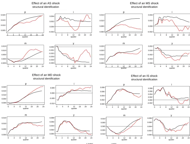
spikiness of the differenced variables, making inference more comfortable. Figure 5 contains
all the IRFs produced under the structural ISLM scheme.
The similarity in the VIRF‘s and LPIRF‘s unaccumulated responses naturally translates into
similarity in their accumulated responses, but with a few interesting exceptions. On the whole,
the results of both techniques seem to uphold the theoretical predictions of the ISLM model.21
There is a strong consensus between techniques concerning MD and IS shocks. The positive
IS shock is normalised to the output equation. After the initial shock, output falls but stays
above the pre-shock level for the full 6 year horizon. The positive IS shock is analogous to
the IS curve shifting outwards in the standard ISLM model, related to an increase of output
and the interest rate. Indeed, the shock is associated with a rise of the interest rate of
approximately 40 basis points, rising to nearly 85 points above the pre-shock level after 18
months. Price and output settle at new higher levels while the interest rate returns to its
pre-shock level.
21 An ordering of the variables was chosen such that the structural shock is relatable to a positive innovation
The positive MD shock is normalised to the money equation so nominal money rises. The
money stock continues to rise at a decreasing rate until 4 years after the shock where it
plateaus at a new higher level. The increased liquidity increases prices with a lag as one
would expect. The shock decreases the interest rate and increases output. As the money level
stabilises, prices continue to rise and the interest rate settles at a new higher level. Output
peaks after 18 months before tending back to its pre-shock level in accordance with notions
of monetary neutrality.
The AS and MS shocks show some differences between the techniques‘ predictions. The AS
shock related to the price equation is associated with a positive reduced form price shock or
adverse AS shock. As expected, both VIRFs and LPIRFs show increasing price and
decreasing output.
The LPIRFs ability to capture fluctuations at longer horizons becomes evident here. The
VIRF for the interest rate‘s response is more or less flat between 20-30 basis points above the
pre-shock level after 18 months. However, the LPIRF darts sharply below the VIRF after 2
years and below the pre-shock level 6 months later. This is particularly interesting because
the divergence in IRFs occurs precisely at the 8th horizon (the VAR‘s order) giving a
structurally meaningful example of the phenomenon discussed in section 5.2.1. Of course, divergence can happen at any time e.g. the LPIRF for output‘s response significantly departs
from that of the VIRF after 4 years.
The tightening MS shock is related to an increase in the interest rate. Output is suppressed
and settles at a new lower level after 2 years, although the LPIRF shows signs of tending
back to the pre-shock level again supporting the notion of monetary neutrality whereas the
VIRF is steady at a new lower level. The positive trend of money and prices is unexpected.
Figure 5 Structural ISLM LPIRFs and VIRFs
0.005 0.010 0.015 0.020
0 4 8 12 16 20 24 quarter p -0.002 0.000 0.002 0.004
0 4 8 12 16 20 24 quarter i -0.005 0.000 0.005 0.010 0.015
0 4 8 12 16 20 24 quarter m -0.005 -0.004 -0.003 -0.002 -0.001 0.000
0 4 8 12 16 20 24 quarter
y structural identification
Effect of an AS shock
0.000 0.005 0.010 0.015
0 4 8 12 16 20 24 quarter p -0.002 0.000 0.002 0.004
0 4 8 12 16 20 24 quarter i 0.005 0.010 0.015 0.020 0.025
0 4 8 12 16 20 24 quarter m -0.006 -0.004 -0.002 0.000 0.002
0 4 8 12 16 20 24 quarter
y structural identification
Effect of an MS shock
0.000 0.005 0.010 0.015 0.020
0 4 8 12 16 20 24 quarter p -0.010 -0.005 0.000 0.005
0 4 8 12 16 20 24 quarter i 0.000 0.005 0.010 0.015
0 4 8 12 16 20 24 quarter m 0.000 0.002 0.004 0.006 0.008
0 4 8 12 16 20 24 quarter
y structural identification
Effect of an MD shock
0.000 0.002 0.004 0.006 0.008
0 4 8 12 16 20 24 quarter p -0.002 0.000 0.002 0.004 0.006 0.008
0 4 8 12 16 20 24 quarter i -0.010 -0.005 0.000 0.005 0.010
0 4 8 12 16 20 24 quarter m 0.000 0.002 0.004 0.006 0.008
0 4 8 12 16 20 24 quarter
y structural identification
falls to fluctuate around the pre-shock level. The VIRF on the other hand shows a much more
gradual decrease in the interest rate, and a monotonic concave path for prices stabilising at a
higher level – a form of the ―price puzzle‖ which has hampered many SVAR applications. Again, the substantial difference of the techniques‘ predictions in the response of prices
occurs approximately at the horizon equal to the VAR‘s lag order.
6) Conclusions
Through a careful selection of identification scheme and an understanding of the VIRF and
LPIRF techniques, we have highlighted the importance to the answer of the question ‗which impulse response function?‘. Combining structural identification and LPIRFs to test the
implications of the ISLM model was an original contribution of this paper, as was the use of
Stata.
Through theoretical and empirical work, this paper has suggested that the bias of VIRFs
becomes more severe at horizons higher than the lag length and that LPIRFs offer a remedy
to this. Divergence of the IRFs often occurs at, or soon after the lag length horizon. It was
then highlighted that even when it is suspected that a VAR process well approximates the
DGP so that both techniques give consistent estimates, the impact of choosing VIRFs or
LPIRFs can have important implications. The ISLM application showed VIRF and LPIRF
techniques produced similar macroeconomic dynamics broadly congruent with theoretical
predictions, but there were some stark differences. The methods have the potential to give
conflicting answers to big questions about both a variable‘s more short-run trends (e.g. the
price-puzzle) and long-run responses (e.g. monetary neutrality). The message from this work
to practitioners is that although relatively new, local projection techniques warrant inclusion
References
Ayat, L., and Burridge, P., 2000, Unit root tests in the presence of uncertainty about the non-stochastic trend, Journal of Econometrics, (95) 71-96.
Balke, N. S., 2010, Sectoral Effects of Aggregate Shocks, Working Paper of the Federal Reserve Bank of Dallas.
Basher, S. A., Haug, A. A., and Sadorsky, P., 2010, Oil Prices, Exchange Rates and Emerging Stock Markets, Working Paper, yet unpublished. Link: http://www.syedbasher.org/wp/Basher&Haug&Sadorsky.pdf
Berg, T. O., 2010,Do Monetary and Technology Shocks Move Euro Area Stock Prices?, MPRA Paper 23973, University Library of Munich.
Bernanke, B. S., 1986, Alternative Explanations of the Money-Income Correlation, Carnegie-Rochester Conference Series on Public Policy, (25) 49-100
Bernanke, B. S., and Blinder, A. S., 1992, The Federal Funds Rate and the Channels of Monetary Transmission, American Economic Review, Vol.82 (4) 901-921.
Blanchard, O. J. and Quah, D., 1989, The Dynamic Effects of Aggregate Demand and Supply Disturbances, NBER Working Paper Series 2737.
Blanchard, O. J., Watson, M. W., 1984, Are Business Cycles All Alike?, NBER Working Paper Series 1392.
Braun, P. A., and Mittnik, S., 1993, Misspecifications in Vector Autoregressions and their Effects on Impulse Responses and Variance Decompositions, Journal of Econometrics, Vol.59 319-341.
Canova, F., de Nicolo, G., 2002. Monetary disturbances matter for business fluctuations in the G-7. Journal of Monetary Economics, Vol.49 (6) 1131–1159.
Canova, F., Pina, J., 1999, Monetary policy misspecification in VAR models, CEPR Discussion Paper 2333.
Christiano, L. J., Eichenbaum, M., and Vigfusson, R. J., 2006, Assessing structural VARs, International Finance Discussion Papers 866.
Cooley, T. F. and LeRoy, S. F., 1985, Atheoretical Macroeconomics: A Critique, Journal of Monetary Economics (16) 283-308.
Cooley, T. F., and Dwyer, M., 1998, Business Cycle Analysis without Much Theory: A Look at Structural VARs. Journal of Econometrics, Vol.83 (1-2) 57-88.
Dupor, B., and Kiefer, L., 2008, Executing Long Run Restrictions, Working Paper of Ohio State University and Texas Tech. University.
Eichenbaum, M., and Evans, C. L., 1995, Some Empirical Evidence on the Effects of Shocks to Monetary Policy on Exchange Rates, Quarterly Journal of Economics, Vol.110 (4) 975-1009
Faust, J., 1998, The Robustness of Identified VAR Conclusions About Money, International Finance Discussion Papers 610.
Faust, J., and Leeper, E. M., 1997, When Do Long-Run Identifying Restrictions Give Reliable Results?, Journal of Business & Economic Statistics, Vol.15 (3) 345-353. Fisher, J. D., 2006, The Dynamic Effects of Neutral and Investment-Specific Technology
Shocks, Journal of Political Economy, Vol.114 (3) 413-51.
Francis, N., and Ramey, V. A., 2004, The Source of Historical Economic Fluctuations: An Analysis using Long-Run Restrictions, NBER Working Paper Series 10631.
Fry, R., and Pagan, A., 2007, Some Issues in Using Sign Restrictions for Identifying Structural VARs, NCER Working Paper Series 14.
Gali, J., 1992, How Well Does the IS-LM Model Fit Postwar U.S. Data?, The Quarterly Journal of Economics, Vol.107 (2) 709-738.
Gerlach, S., and Smets, F., 1995, The Monetary Transmission Mechanism: Evidence From the G-7 Countries, Bank for International Settlements Working paper No.26.
Hall, A., Inoue, A., Nason, J. M., and Rossi, B., 2007, Information Criteria for Impulse Response Function Matching Estimation of DSGE Models, Duke University Working Paper 07-04.
Hamilton, J. D., 1994, Time Series Analysis, Princeton University Press.
Haug, A. A., and Smith, C., 2007, Local Linear Impulse Responses for a Small Open Economy, University of Otago Economics Discussion Paper 0707.
Herwartz, H., and Lütkepohl, H., 2010, Structural Vector Autoregressions with Markov Switching: Combining Conventional with Statistical Identification of Shocks, European University Institute Conference Paper, yet unpublished. Link: http://www.eui.eu/Documents/DepartmentsCentres/Economics/Researchandteaching/ Conferences/2010Conferences/Luetkepohlpaper.pdf
Ho, T. W., 2008, On the Dynamic Relationship of Exchange Rates and Monetary Fundamentals: an Impulse-Response Analysis by Local Projections, Applied Economics Letters, Vol.15 (14) 1141 — 1145.
Jordà, Ò., 2005, Estimation and Inference of Impulse Responses by Local Projections, American Economic Review, Vol. 95 (1) 161-182.
Jordà, Ò., 2007, Joint Inference and Counterfactual Experimentation for Impulse Response Functions by Local Projections, University of California (Davis) Working Paper Series 06-24.
Jordà, Ò., 2009, Simultaneous Confidence Regions for Impulse Responses, Review of Economics and Statistics, Vol.91 (3) 629-647.
Jordà, Ò., and Marcellino, M., Path Forecast Evaluation, Journal of Applied Econometrics, Vol.25 635-662.
Keating, J. W., 1992, Structural Approaches to Vector Autoregressions, Federal Reserve Bank of St. Louis Review, Vol.74 (5) 37-57.
Kilan, L., and Kim, Y. J., 2009, Do Local Projections Solve the Bias Problem in Impulse Response Inference?, CEPR Discussion Paper Series 7266.
Kilian, L., 1998, Small-Sample Confidence Intervals for Impulse Response Functions, The Review of Economics and Statistics, Vol.80 (2) 218-230.
Kilian, L., 2001, Impulse Response Analysis in Vector Autoregressions with Unknown Lag Order, Journal of Forecasting, Vol.20 161-179.
King, R. G., Plosser, C. I., Stock, J. H., & Watson, M. W., 1991, Stochastic Trends and Economic Fluctuations, American Economic Review, Vol.81 (4) 819-840.
Lastrapes, W. D., and Selgin, G., 1995, The Liquidity Effect: Identifying Short-Run Interest Rate Dynamics Using Long-Run Restrictions, Journal of Macroeconomics, Vol.17 (3) 387-404.
Lütkepohl, H., 1990, Asymptotic Distributions of Impulse Response Functions and Forecast Error Variance, The Review of Economics and Statistics, Vol.72 (1) 116-125.
Lütkepohl, H., 2005, Introduction to Multiple Time series analysis, Springer.
Lütkepohl, H.,2009, Forecasting Aggregated Time Series Variables: A Survey, European University Institute, Working Paper Series ECO 2009/17.
Mamoudou, T., Jamel, T., Dufourt, F., 2009, Empirical evaluation of nominal convergence in Czech Republic, Poland and Hungary, Economic Modelling, (26) 993-999.
McMillin, W. D., 2001, The Effects of Monetary Policy Shocks: Comparing Contemporaneous versus Long-Run Identifying Restrictions, Southern Economic Journal, Vol. 67 (3) 618-636.
Pagan, A., 1987, Three Econometric Methodologies: A Critical Appraisal, Journal of Economic Surveys, Vol.1 (1) 3-24.
Palm, F., and Zellner, A., 1974, Time Series Analysis and Simultaneous Equation Econometric Models, Journal of Econometrics, Vol.2 (1) 17-54.
Peersman, G., 2005, What Caused the Early Millennium Slowdown? Evidence Based on Vector Autoregressions, Journal of Applied Econometrics, Vol.20 (2) 185–207.
Peersman, G., and Smets, F., 2001, The Monetary Transmission Mechanism in the Euro Area: More Evidence from VAR Analysis, European Central Bank Working Paper No.91. Peersman, G., and Straub, R., 2009, Technology Shocks and Robust Sign Restrictions in a
Euro Area SVAR, International Economic Review, Vol.50 (3) 727-750.
Shapiro, M. D. and Watson, M. W., 1988, Sources of Business Cycle Fluctuations, NBER Macroeconomics Annual, (3) 111-148.
Sims, C. A., and Zha, T., 2006, Were There Regime Switches in U.S. Monetary Policy?, American Economic Review, Vol.96 (1) 54-81.
Sims, C. A., 1980, Macroeconomics and Reality, Econometrica, Vol.48 (1) 1-48.
Sims, C. A., 1986, Forecasting and Conditional Projection Using Realistic Prior Distribution, Federal Reserve Bank of Minneapolis Staff Report 93.
Stata Programming Reference Manual Release 9, 2005, College Station. Stata Time Series Reference Manual Release 9, 2005, College Station.
Stock, J. H. and Watson, M. W., 1999, A Comparison of Linear and Nonlinear Univariate Models for Forecasting Macroeconomic Time Series, in Cointegration, Causality, and Forecasting - Festschrift in Honour of Clive W. J. Granger, edited by Engle, R., and White, H., Oxford University Press.
Stock, J. H., and Watson, M. W., 2001, Vector Autoregressions, The Journal of Economic Perspectives, Vol.15 (4) 101-115.
Taylor, M. P., 2004, Estimating Structural Macroeconomic Shocks Through Long-Run Recursive Restrictions on Vector Autoregressive Models: The Problem of Identification, International Journal of Finance and Economics, (9) 229-244.
Uhlig, H., 2005, What Are the Effects of Monetary Policy on Output? Results From an Agnostic Identification Procedure, Journal of Monetary Economics, Vol.52 381–419. Wallis, K. F., 1977, Multiple Time Series and the Final Form of Econometric Models,
Econometrica, Vol.45 (6), 1481-97.
Weiss, Andrew A., 1991, Multi-Step Estimation and Forecasting in Dynamic Models, Journal of Econometrics, Vol.48 (1-2) 135-49.
Appendix
Table A.1 – Augmented Dickey Fuller (ADF) Unit Root Tests
Variable Lag Length for ADF test Lag Length Selection Criteria in agreement
Approximate
p-value Conclusion
6* FPE, AIC, HQIC 0.9839 ( )
5* FPE, AIC, HQIC 0.0266 ( )
5* LR, HQIC 0.0314 ( )
8* FPE, AIC 0.9075 ( )
7 LR, FPE, AIC 0.0033 ( )
2* FPE, AIC, HQIC, SBIC 0.0574 ( )
11 LR, FPE, AIC 0.0003 ( )
1) FPE – final prediction error, AIC – Akaike‘s information criterion, SBIC – Schwarz Bayesian IC, HQIC – Hannan Quinn IC, LR – sequential likelihood ratio test recommendation.
2) Where there is profound disagreement amongst the criteria for lag length, then the higher of the indicated lengths is chosen. If too low, misspecification causes the Dickey Fuller distribution to be invalidated, and inference incorrect due to the serially correlated errors. If too high, we lose some power of the test, which is inefficient compared to the correct specification. I made the judgement call that getting the number of lags too high rather than too low seems a more reasonable inaccuracy.
3) * means that the test was performed with a linear trend as an exogenous variable. Basic visual interpretation leads to the final inclusion of trends. All tests bar (and ) were invariant to trend inclusion, so no further mention is necessary. Without a trend ( ) reported an approx. p-value of 0.0546 (0.0505), borderline for rejection of it being I(1). To discover if ( ) has a trend or not, Ayat and Burridge‘s (2000) sequential procedure is followed, and we find evidence for trend inclusion, so that the reported approx. p-value is appropriate.
Table A.2 – Lag Length Selection Criteria
Lag FPE AIC HQIC SBIC
0 6.00E-16 -23.698 -23.668 -23.623
1 2.20E-17 -27.018 -26.867 -26.646*
2 1.90E-17 -27.173 -26.901 -26.504
3 1.50E-17 -27.389 -26.997* -26.422
4 1.30E-17 -27.501 -26.988 -26.237
5 1.30E-17 -27.554 -26.921 -25.992
6 1.30E-17 -27.570 -26.815 -25.710
7 1.20E-17* -27.592* -26.716 -25.435
8 1.30E-17 -27.577 -26.581 -25.123
9 1.40E-17 -27.459 -26.342 -24.707
10 1.40E-17 -27.493 -26.255 -24.443
11 1.40E-17 -27.482 -26.124 -24.135
[image:39.595.163.430.82.303.2]12 1.50E-17 -27.435 -25.956 -23.791
Table A.3 – LM Tests for Serial Correlation
VAR with 7 lags VAR with 8 lags
Lag Chi-Squared
test stat p-value
Chi-Squared
test stat p-value
1 24.73 0.075 7.40 0.965
2 18.53 0.294 14.30 0.577
3 18.41 0.300 20.22 0.211
4 22.82 0.119 20.66 0.192
5 23.68 0.097 23.18 0.109
6 21.66 0.155 20.16 0.213
7 15.14 0.515 9.31 0.900
8 25.12 0.068 20.21 0.211
H0 : No autocorrelation at lag order
Figure A.4 – Roots of the Characteristic Equation
-1
-.
5
0
.5
1
Ima
g
in
a
ry
-1 -.5 0 .5 1
Real
[image:39.595.161.432.407.752.2]