Comparing distributions using dependent normalized random measure mixtures

University of Warwick institutional repository: http://go.warwick.ac.uk/wrap

This paper is made available online in accordance with

publisher policies. Please scroll down to view the document

itself. Please refer to the repository record for this item and our

policy information available from the repository home page for

further information.

To see the final version of this paper please visit the publisher’s website

.

Access to the published version may require a subscription.

Author(s): JE Griffin, M Kolossiatis and MFJ Steel

Article Title: Comparing Distributions Using Dependent Normalized

Random Measure Mixtures

Year of publication: 2010

Link to published article:

http://www2.warwick.ac.uk/fac/sci/statistics/crism/research/2010/paper

10-24

Comparing Distributions Using Dependent Normalized

Random Measure Mixtures

∗

J.E. Griffin

University of Kent, Canterbury, UK

M. Kolossiatis

Cyprus University of Technology, Limassol, Cyprus

M.F.J. Steel

University of Warwick, Coventry, UK

December 15, 2010

Abstract

A methodology for the simultaneous Bayesian nonparametric modelling of several

dis-tributions is developed. Our approach uses normalized random measures with independent

increments and builds dependence through the superposition of shared processes. The

proper-ties of the prior are described and the modelling possibiliproper-ties of this framework are explored in

some detail. Efficient slice sampling methods are developed for inference. Various posterior

summaries are introduced which allow better understanding of the differences between

distri-butions. The methods are illustrated on simulated data and examples from survival analysis

and stochastic frontier analysis.

Keywords: Bayesian nonparametrics; Dependent distributions; Dirichlet process; Normalized

Generalized Gamma process; Slice sampling; Utility function

∗_{Address for correspondence: M. Steel, Department of Statistics, University of Warwick, Coventry CV4 7AL, UK.}

1

Introduction

This paper considers the nonparametric modelling of data divided into different groups and the

comparison of their distributions. For example, we may observe the results of different

med-ical treatments or the performance of firms with different management structures. Statistmed-ical

analysis will often concentrate on inference about the differences in the distributions.

Analy-sis of Variance (ANOVA) concentrates on differences between means for different groups and

links these to the effects of each factor. However, differences between groups may not be well

modelled by restricting attention to location. For example, if there are distinct subpopulations

within the observations then each group may contain different proportions of each

subpopu-lation and a full summary of the differences would involve identifying parts of the support

on which the two distributions place substantially different masses. We follow a full Bayesian

analysis by firstly placing a prior on the distributions and secondly defining a decision problem

which reports where the distributions are similar or substantially different.

We use a Bayesian nonparametric mixture model approach to understand the differences

between the distributions. LetF1, F2, . . . , Fqbe the distribution of observations forqdifferent groups, then an infinite mixture model assumes that the density for theg-th group is

fg=

Z

k(·|θ)dGg(θ)

wherek(·|θ)is a density parameterized byθandGg is a discrete random probability measure. Since the measure is discrete, it can be represented as

Gg =

∞

X

i=1

wg,iδθg,i

whereδxis the Dirac delta function that places mass 1 atxandθg,1, θg,2, . . . andwg,1, wg,2, . . .

are infinite sequences of random variables for whichP∞

i=1wg,i = 1andwg,i >0for alli. It follows that the mixture model can be written as

∞

X

i=1

wg,ik(·|θg,i) (1) or, alternatively, the model can be represented hierarchically for an observation yg,j drawn fromFg as follows

yg,j ∼k(·|θg,sg,j), p(sg,j =i) =wg,i

group. This is a very general model and many previously proposed models fall within it. The

ANOVA-DDP model of De Iorio et al. (2004) assumes that the densitykis a N(θ, σ2_{), while} wg,i =wiand θg,i = zgTβi whereβi is a vector of parameters. This allows the means of the different components to change with covariates.

A popular approach allows the weights to depend on covariates and setsθg,i =θiso that the location of the components is fixed across each group. A finite mixture of normals model

along these lines was proposed by Rodriguez et al. (2009) who allow the component weights

to depend on covariates. Alternatively, the weights can be modelled through combinations of

random variables, which encourages correlation between the random distributions. The Matrix

Stick-Breaking process of Dunson et al. (2008) assumes thatzg is a two-dimensional vector and thatwg,1, wg,2, wg,3, . . . are derived using a Matrix Stick-Breaking construction where

wg,j =Vzg,1,1Vzg,2,2

andV1,1, V2,1, V3,1, . . . andV1,2, V2,2, V3,2, . . . are infinite sequences of beta random variables. M¨uller et al. (2004) assume that

fg =ψ

∞

X

i=1

w_g,i⋆ k(·|θ_g,i⋆ ) + (1−ψ)

∞

X

i=1

wik(·|θi)

where0 ≤ ψ ≤ 1. The distribution of theg-th group is a mixture of a common component shared by all groups and an idiosyncratic component. The parameterψis the weight placed on the idiosyncratic component and so affects the correlation between distributions.

The Hierarchical Dirichlet process (Teh et al., 2006) assumes, in its simplest form, that

Gg ∼DP(M G0), g= 1, . . . , q, G0 ∼DP(M0H) (2)

The distributions are exchangeable and this structure allows clusters to be shared by different

groups (due to the discrete nature of the Dirichlet process at both levels). If the

Hierarchi-cal Dirichlet process is used as the mixture distribution in the mixture models then we have

something of the form of (1). Teh et al. (2006) derive the stick-breaking construction for

wg,1, wg,1, wg,2, . . .. The model can be extended to more levels of hierarchy in the standard

way. This model assumes that distributions are exchangeable at some level. In contrast, this

paper will mostly concentrate on the problem where groups are defined by covariates. There

is normally no natural nesting in these settings, so that hierarchical models will then not be

appropriate.

We propose to use a normalized superposition of random measures to induce dependence.

through the mass parameters of the underlying measures and extends naturally to any number

of groups. In fact, we can use this framework to separately model the mass shared by any

subset of the groups or we can use simpler settings, depending on the flexibility of the

depen-dence structure we want to assume. We use shrinkage priors for the mass parameters to ensure

consistent priors across different levels of model complexity. For posterior inference, we

pro-pose novel slice sampling Markov chain Monte Carlo (MCMC) methods, used in combination

with a split-merge move. We also discuss ways of summarizing the differences between the

nonparametric distributions for each group, based on decision theoretic ideas.

The paper is organized as follows. Section 2 describes the construction of random

proba-bility measures by normalization and our proposed framework for modelling dependence using

normalized random measures, Section 3 describes efficient MCMC sampling methods for

in-ference, Section 4 discusses a decision theoretic approach to comparing distributions, Section

5 analyzes simulated data and presents real data applications to stochastic frontier analysis and

health, while Section 6 concludes.

2

Introducing Dependence in Normalized Random

Mea-sures

2.1

General Framework

Normalized Random Measures with Independent Increments (NRMIs) are a class of

nonpara-metric priors for a random probability measure,G, constructed by normalizing a positive ran-dom measure with independent increments,G˜(B), to give

G(B) = G˜(B) ˜

G(Ω).

Throughout the paper we will useGto represent the normalized version of a random measure

˜

G. Generally, we will concentrate on random measures which only contain jumps and write

˜

G=

∞

X

i=1 Jiδθi,

whereθi are i.i.d. from some distribution Hand J1, J2, J3, . . . are jumps of a L´evy process

with L´evy densityζ(x). The process is well-defined if0 <G˜(Ω) <∞almost surely which happens ifR ζ(x)dxis infinite. The NRMI can be employed as the prior of the mixing measure

Gin an infinite mixture modelf(y) =R

of processes and their use in mixture models is studied in general by James et al. (2009).

Several previously proposed processes fall within this class. The Dirichlet process (Ferguson,

1973) (DP) occurs ifG˜is a Gamma process, for which

ζ(x) =M x−1exp{−x}, M >0.

The Normalized Generalized Gamma process (Lijoi et al., 2007) (NGG) is constructed by

normalizing a Generalized Gamma process (Brix, 1999), for which

ζ(x) = M Γ(1−a)x

−1−a_{exp{−λx}, M >0, 0< a <1, λ≥0. (3)} This process tends to the Dirichlet Process as a → 0and λ = 1. The Normalized Inverse-Gaussian process (Lijoi et al., 2005) occurs ifa= 0.5andλ= 1. Another special case is the Normalized Stable Process of Kingman (1975), which corresponds toλ= 0.

Dependence between two distributions G1 andG2 can be introduced through the unnor-malized random measuresG˜1 andG˜2. Intuitively, it is clear that the dependence betweenG1

andG2will grow as the dependence between G˜1 andG˜2 grows. A similar approach for

con-structing processes of random probability measures over time is discussed by Griffin (2009).

Suppose that we haveqgroups, then the random measures can be defined in the following way. Firstly, we can definepunderlying random measuresG˜⋆

1,G˜⋆2, . . . ,G˜⋆psuch that

˜

G⋆_j =

∞

X

i=1

Jj,iδθj,i, j= 1, . . . , p,

where θj,i are i.i.d. from some distribution H and Jj,1, Jj,2, Jj,3, . . . are jumps with L´evy

densityζ⋆

j(x). DefiningG˜⋆ = ( ˜G⋆1,G˜⋆2, . . . ,G˜⋆p)T, the random measures in the vectorG˜ =

( ˜G1,G˜2, . . . ,G˜q)T will be formed as

˜

G=DG˜⋆,

whereDis aq×p-dimensional selection matrix. ThenG˜j is a L´evy process and the L´evy den-sity ofG˜jisζj(x) =Dj·ζ⋆(x)whereDj·is thej-th row ofDandζ⋆(x) = (ζ1⋆(x), . . . , ζp⋆(x))T. In particular, we takeζ⋆

h(x) =Mhη(x)so thatζj(x) = [Dj·M]η(x)whereM = (M1, . . . , Mp)T. When we normalize, we obtain

G=W G⋆, (4)

whereG= (G1, . . . , Gq)T,G⋆ = (G⋆₁, . . . , G⋆p)T andW is aq×pmatrix with elements

Wij =

DijG˜⋆j(Ω)

Pp

k=1DikG˜⋆k(Ω)

andG⋆_j = ˜

G⋆ j

˜

G⋆ j(Ω)

Therefore, the distribution for each group is a mixture ofG⋆

1, G⋆2, . . . , G⋆pwhere the weights for thei-th group are given by thei-th row ofW. This process will be denoted generally as a Cor-related Normalized Random Measure with Independent Increments, or CNRMI(M, H, D;η). Often, we will choose a specific functional form forηso that the marginal processesG1, . . . , Gq come from a known process (for example, a Dirichlet process). We will consider two

pos-sibilities: a Correlated Dirichlet Process CDP(M, H, D) where η(x) = x−1exp{−x} and the marginal processes are DP and a Correlated Normalized Generalized Gamma Process

CNGG(M, H, D;a, λ)whereη(x) =x−1−a_{exp{−λx}and the marginal processes are NGG.} The mixture form forG1, G2, . . . , Gq is an important difference to the Hierarchical Dirichlet process, which is a framework that leads to all atoms being shared by all distributions and

assumes that all distributions are a priori equally correlated.

If we useG1, G2, . . . , Gq as mixing measures forqmixture models, the distribution of an observation,y, in thei-th group is now given by

fi(y) =

Z

k(y|θ)dGi(θ). Then we can write

fi=

˜

fi

˜

Fi(Ω)

,

wheref˜i(y) =

R

k(y|θ)dG˜i(θ)andF˜i(A) =

R

Af˜i(y)dy. Now,F˜iexpresses an unnormalized distribution in terms of basis functions (where the kernelk(·)are the basis functions) and so

Fi is a normalized basis function model.

A natural measure of the dependence between two distributions is the correlation between

Gi(B) and Gj(B) where B is a measurable set. Using the construction in this paper, this correlation does not depend on B and so can be used as a single measure of dependence between distributions, which we denote by Corr(Gi, Gj). The following results present an expression for the correlation, using a particular form of the framework described above for

q= 2,p= 3andD=





1 1 0 1 0 1



. This is a simple, yet illustrative example.

Theorem 1 Suppose thatG˜1 = ˜G⋆1+ ˜G⋆2andG˜2 = ˜G⋆1+ ˜G⋆3 where the L´evy measure ofG˜⋆k isMkη(x). Define

Lη(v) =

Z ∞

0

(1−exp{−vx})η(x)dx.

The covariance ofG1andG2 is

Cov(G1(B), G2(B)) =H(B)(1−H(B))M1 Z ∞

0 Z ∞

0

where

β(v1, v2;M1, M2, M3) =−L′′η(v1+v2) exp{−M1Lη(v1+v2)−M2Lη(v1)−M3Lη(v2)}.

Proof: See Appendix

Similarly, expressions can be derived for Var(G1(B))and Var(G2(B))and so

ρ=Corr(G1, G2) =

M1 R∞

0 R∞

0 β(v1, v2;M1, M2, M3)dv1dv2 p

(M1+M2)(M1+M3)β∗(M1+M2)β∗(M1+M3) ,

where

β∗(M) =

Z ∞

0 Z ∞

0

−L′′_η(v1+v2) exp{−M Lη(v1+v2)} dv1dv2.

In the special case whereM1=M ρ⋆andM2 =M3 =M(1−ρ⋆)for0< ρ⋆ <1, we obtain ρ=ρ⋆[1 +ǫ],

where

ǫ=

R∞ 0

R∞

0 −L′′η(v1+v2) exp{−M Lη(v1+v2)}γ(v1, v2)dv1dv2

β∗_(M) ,

with

γ(v1, v2) = exp{−M(1−ρ⋆) [Lη(v1) +Lη(v2)−Lη(v1+v2)]} −1.

Therefore, the correlation betweenG1andG2,ρ, can be well-approximated byρ⋆ ifγ(v1, v2)

is close to zero for allρ⋆ which will be the case for many forms of processes. It is impor-tant to point out we do not necessarily advocate adopting the restricted parametrization for

M1, M2 andM3 in the special case used above, but it is a useful device to better understand

the properties of our models, as illustrated in the following examples:

Dirichlet process marginals (CDP)

Here

Lη(v) = log(1 +v), L′′η(v) =−

1 (1 +v)2,

so that

γ(v1, v2) = exp

−M(1−ρ⋆) log

1 + v1v2 1 +v1+v2

−1.

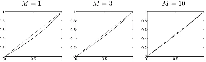
Figure 1 plots the correlation betweenG1andG2as a function ofρ⋆and illustrates thatρ⋆

M = 1 _M = 3 _M = 10

0 0.5 1

0 0.2 0.4 0.6 0.8 1

0 0.5 1

0 0.2 0.4 0.6 0.8 1

0 0.5 1

0 0.2 0.4 0.6 0.8 1

Figure 1:Plot of the actual correlation,ρ, (solid line) andρ⋆_{(dashed line) againstρ}⋆_{for the CDP.}

Normalized Generalized Gamma process marginals (CNGG)

In this case

Lη(v) =

1

a((v+λ)

a_−λa_{), L}′′

η(v) = (a−1)(v+λ)a−2, which implies that

γ(v1, v2) = exp

−M(1−ρ⋆)1

a[(v1+λ)

a

+ (v2+λ)a−(v1+v2+λ)a−λa]

−1.

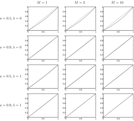
Figure 2 shows the relationship between ρ⋆ _{and the actual correlation, ρ, for CNGG} pro-cesses with different choices of the parameters. The correlation is close toρ⋆for each choice of the hyperparameters with the largest differences for the smaller values ofaandλ. For gen-eralM1,M2 andM3, this results suggests that increasingM1relative toM2 andM3leads to

a larger correlation betweenG1andG2.

Whenq > 2, we can always write a pair of unnormalized distribution G˜j and G˜k, where

j6=k, as

˜

Gj = ˜G(c)+ ˜G(j)

˜

Gk= ˜G(c)+ ˜G(k),

where, using I(·) to denote the indicator function, the L´evy measure of G˜(c) _{is given by}

[Pp

m=1I(Djm= 1, Dkm = 1)Mm]η(x),G˜(j)has L´evy measure[Ppm=1I(Djm = 1, Dkm=

0)Mm]η(x)andG˜(k)has L´evy measure[

Pp

m=1I(Djm= 0, Dkm = 1)Mm]η(x). This sug-gest using the general approximation

Corr(Gj, Gk)≈

M(c) p

M(c)_+M(j)p_M(c)_+M(k), (5)

where M(c) ₌ Pp

m=1I(Djm = 1, Dkm = 1)Mm, M(j) = Ppm=1I(Djm = 1, Dkm =

M = 1 _M = 3 _M = 10

a= 0_.5_{, λ}= 0

0 0.5 1

0 0.2 0.4 0.6 0.8 1

0 0.5 1

0 0.2 0.4 0.6 0.8 1

0 0.5 1

0 0.2 0.4 0.6 0.8 1

a= 0_.9_{, λ}= 0

0 0.5 1

0 0.2 0.4 0.6 0.8 1

0 0.5 1

0 0.2 0.4 0.6 0.8 1

0 0.5 1

0 0.2 0.4 0.6 0.8 1

a= 0_.5_{, λ}= 1

0 0.5 1

0 0.2 0.4 0.6 0.8 1

0 0.5 1

0 0.2 0.4 0.6 0.8 1

0 0.5 1

0 0.2 0.4 0.6 0.8 1

a= 0_.9_{, λ}= 1

0 0.5 1

0 0.2 0.4 0.6 0.8 1

0 0.5 1

0 0.2 0.4 0.6 0.8 1

0 0.5 1

0 0.2 0.4 0.6 0.8 1

Figure 2: Plot of the actual correlation,ρ, (solid line) andρ⋆(dashed line) againstρ⋆for the CNGG.

Gj and Gk increases as the value of M(c) increases relative to M(j) and M(k). Generally, increasing Mh leads to increased correlations between all distributions with a 1 in the h-th column ofD.

2.2

Modelling of Groups

In the simple case with 2 groups, there are naturally three underlying random measures G˜⋆ j

in our model, one modelling the common mass shared between the groups and two for the

idiosyncratic components. In cases with more groups, we need to make modelling decisions,

allocating a separate random measure for modelling the mass shared by each nonempty subset

of group distributions. The most complete model forqgroups in the CRNMI class with a given

M,Handηcan thus be defined by takingp= 2q_{−1and letting thei-th column ofDbe the} binary representation ofifor1≤i≤2q_{−1. For example ifq= 3, then}

D=



  

0 0 0 1 1 1 1 0 1 1 0 0 1 1 1 0 1 0 1 0 1



  

whereG˜⋆₁,G˜⋆₂andG˜⋆₄are idiosyncratic components,G˜⋆₃,G˜⋆₅andG˜⋆₆are shared by two groups and G˜⋆

7 is shared by all three groups. This will be called the saturated model. The levels of

correlation between the distributions can be accommodated by choosing appropriate values

of M1, . . . , Mp and using (5). Clearly this model becomes increasingly complicated as q increases. More parsimonious models can be constructed by removing columns of Dfrom the saturated model (which is equivalent to setting someMh to zero). A version of the model introduced by M¨uller et al. (2004) would use theq×(q+ 1)-dimensional matrix

D= (1_{q Iq),}

where1_{qis aq-dimensional vector of ones (representing the single common component) andIq}

is theq×q-dimensional identity matrix. Alternatively, if the distributions relate to observations at different times then a simple model could be defined using

D= (1_{q Iq F),}

whereF is aq×(q−1)-dimensional matrix for which

Fij =

 



1 ifj=iorj=i−1

0 otherwise .

The model then includes a common underlying measure (in the first column), idiosyncratic

underlying measures (in the nextqcolumns) and underlying random measures shared by con-secutive distributions (in the next q −1 columns). More specific form of problem-specific dependence could also be modelled. Suppose that we take observations from three

distribu-tions where we think that distribution 1 and 2 are more related to each other than to distribution

3. A suitable model would be

D=



  

1 1 0 0 1 1 0 1 0 1 1 0 0 1 0



where the inclusion of the final column allows extra dependence between the first two

distri-butions.

In practice, we may not have prior information that leads us to consider models simpler than

the saturated model. We suggest using regularization to avoid overfitting (since the number

of underlying processes, p, grows quickly with q). A standard approach would be Bayesian variable selection on the columns ofDfor the saturated model. This is equivalent to setting

Mh = 0 in the L´evy measure of the underlying measure G˜⋆h. We will take an alternative approach and define a prior forMhwhich encourages substantial shrinkage towards zero (this is similar to the shrinkage prior approach to regression as described by Scott and Polson (2011)

and Griffin and Brown (2010)). The prior for M1, M2, . . . , Mp is chosen in the following way. The values ofM1, M2, . . . , Mpcontrol the dependence between distributions and can be chosen to represent prior beliefs. The additive effect of theM_j′s is useful here. Suppose that we

0 0.5 1

0 1 2 3 4

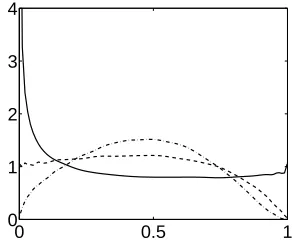
Figure 3: The prior onρ =Corr(G1, G2)withMi ∼Ga(M∗/2, β)whereM∗ = 1(solid line),M∗ = 2 (dashed line) andM∗ _{= 3(dot-dashed line) andβ= 1.}

have one distribution withM chosen to take the valueM∗. Moving to two distributions in the saturated model suggests thatM1+M3=M∗andM2+M3 =M∗, if we assume thatG1and G2are exchangeable, so that we haveM1=M2. If we are indifferent between an observation

being allocated to a shared cluster or an idiosyncratic cluster thenM1 =M2 =M3. Repeated

use of this argument allows extension to any value ofqand suggests thatM1, M2, . . . , Mpare independent andMi ∼ Ga(M∗/2q−1, β). Figure 3 shows the prior distribution induced on

ρ, the correlation coefficient betweenG1 andG2 whenq = 2, for various values ofM∗. All priors are centred around 1/2 with the variability decreasing as M∗ _{increases. We will use}

3

Computational Methods

This section describes an MCMC sampler for fitting the general mixture model

yg,i ∼k(yg,i|θg,i), i= 1,2, . . . , ng

θg,i ∼Gg

G1, G2, . . . , Gq∼CNRMI(M, H, D;η)

whereMis given the prior described in Section 2 andHandηpotentially have hyperparame-ters which also have priors.

Several slice sampling algorithms for normalized random measure mixture models were

introduced by Griffin and Walker (2010). We will extend their “Slice 1” algorithm. For a

single normalized random measure mixture the posterior is proportional to

p(J)p(θ)

n

Y

i=1

wsik(yi|θsi)

wherewi = Ji/P∞l=1Jl, J = (J1, J2, J3, . . .)and θ = (θ1, θ2, θ3, . . .). They demonstrate

that the following posterior with additional auxiliary variablesu1, u2, . . . , unandv1, v2, . . . , vn and integrating over all jumps smaller thanL = min{ui}is a much simpler form for compu-tational purposes:

p(J1, J2, . . . , JK)p(θ) n

Y

i=1

I(ui < Jsi) exp

(

−vi K

X

l=1 Jl

)

E

"

exp

(

−vi

∞

X

l=K+1 Jl

)#

k(yi|θsi)

whereJ1 > J2 > J3 > ... > JK > L, u1, u2, . . . , un > 0 and v1, v2, . . . , vn > 0. The expectation can be evaluated using the L´evy-Khintchine formula and so

E

"

exp

(

−v

∞

X

i=K+1 Ji

)#

= exp

−M Z L

0

(1−exp{−vx})η(x)dx

.

The integral in the exponential is sometime available in terms of special function (this is the

case for the Dirichlet process) or can be evaluated using standard quadrature methods.

The likelihood for a mixture model using the weights in Section 2 can be expressed in

a suitable form for computation by introducing latent variables {sj,i}j=1:q,i=1:nj which are

allocation variables for mixture components while{rj,i}j=1:q,i=1:njallocates each observation

to be drawn fromk(·|θrg,i,sg,i). Using auxiliary variablesuj,1, . . . , uj,nj andvj,1, . . . , vj,njfor

groupj, the likelihood can now be expressed as

p(θ)

q

Y

i=1 Vni−1

i p

Y

i=1

p(Ji,1, Ji,2, . . . , Ji,Ki)

q Y j=1 nj Y i=1

I uj,i< Jrj,i,sj,i

expn−VTDJ(+)o

×Ehexpn−VTDJ(∞)oi, (6)

where Ji,1 > Ji,2 > Ji,3 > . . . for all i, θ = {θi,j}i=1:p,j=1,2,3,... and Ji,1, . . . , Ji,Ki

are all jumps in process G˜⋆

i which are larger than L. V is a q-dimensional vector where

Vj = P nj

i=1vj,i, J(+) is a p-dimensional vector with J (+)

i =

PKi

l=1Ji,l and J(∞) is a p -dimensional vector whereJ_i(∞) =P∞

l=Ki+1Ji,l. Integrating outuj,ifrom (6), the likelihood

can be expressed as

p(θ)

q

Y

i=1 Vni−1

i p

Y

i=1

p(Ji,1, Ji,2, . . . , Ji,Ki)

p Y j=1 Kj Y i=1 Jnj,i

j,i exp

n

−VTDJ(+)o

×E

h

expn−VTDJ(∞)oi,

wherenj,i= #{(l, k)|sl,k =iandrl,k=j, 1≤k≤nl,1≤l≤q}is the size of the cluster of observations associated withθj,i.

Each expectation in the product can be evaluated using the L´evy-Khintchine formula and

so

E

h

expn−VTDJ(∞)oi= expn−1T

pM˜E˜

o ,

whereM˜ is ap×p-diagonal matrix withM˜hh=Mh and, definingD·ias thei-th column of

D,E˜is thep-dimensional vector withi-th element

˜

Ei =

Z L

0

1−exp

−VTD·ix η(x)dx.

Therefore the posterior retains a lot of the linearity introduced in the model. The chain can

be initialized in the following way. Choose a starting truncation point Land generatep dif-ferent Poisson processes where the number of jumps, Kj, in the j-th process is simulated from a Poisson distribution with mean Mj

R∞

L η(x)dx. The jumps of the j-th process are simulated by first drawing Kj random numbers {ξj,k}

Kj

k=1 from a uniform distribution

be-tween 0 and R_L∞η(x)dx and ordered so that ξj,1 < ξj,2 < . . . < ξj,Kj and then setting

Jj,k =Q−1(ξj,k)fork= 1,2, . . . , Kj whereQ−1is the inverse ofQ(x) =

R∞

x η(y)dy. The locationsθj,1, θj,2, . . . , θj,Kj are taken to be i.i.d. fromH and the latent variablesrj,iandsj,i

can be simulated from the discrete distributions

p(rj,i =k) =

DjkMk

Pp

l=1DjlMl

and

p(sj,i=k)∝k yi|θrj,i,k

Jrj,i,k, 1≤k≤Krj,i.

The slice latent variables can be taken asuj,i ∼U(L, Jrj,i,sj,i).

In the following steps, we defineJ_j∗={Jj,i|nj,i6= 0}, i.e. the jumps in thej-th component process which have observations allocated to them. The steps of the Gibbs sampler are as

follows:

Step 1: Split-Merge move

The problem of multi-modality of the posterior distribution in these models and a

computa-tional solution, a split-merge move, are described in Kolossiatis et al. (2010). In our model, it

is useful to link the underlying measures to their corresponding columns in theDmatrix. For example, in the saturated model withq = 3 described at the start of Subsection 2.2, the un-derlying random measureG˜⋆

1will be referred to as the “underlying random measure(0,0,1)”.

The split-merge move is performed in the following way. A split move is selected with

prob-ability 1/2, otherwise a merge move is proposed. An underlying random measuree_{, a column}

ofD, is selected at random from those underlying random measures which have observation allocated to them and a non-empty mixture component, i⋆_{, from e is selected uniformly at} random. If the split move is selected, the members of the cluster are divided according to

their group membership into two clusterse_1ande_{2. For example, in the saturated model with}

q = 3, if we choose e _{= (1,1,0) the cluster would be split into a cluster in the underlying}

measure(1,0,0) and a cluster in the underlying measure(0,1,0). In this case, there is only one possible split. However, if we choosee_{= (1,1,1), there are three possible splits: clusters}

in(1,0,0) and (0,1,1), clusters in(0,1,0) and(1,0,1), or clusters in(0,0,1) and(1,1,0). The particular split is chosen uniformly at random from all possible splits. The merge move

performs the opposite operation. For this move, a set of allowable underlying measures is

defined, C = {e⋆_|e⋆

j = 0for alljfor whichej = 1}, and an underlying measure e†is cho-sen uniformly at random fromC(this happens regardless of whether there are any non-empty

clusters allocated to that measure). One of the non-empty clusters, j⋆_{, ine}† _{(if any exist) or}

a “null” cluster is chosen at random with equal probability. A new cluster is then formed in

the underlying random measureecomb _whereecomb_{i = 1if}e⋆_{i = 1or}e†

i = 1and ecombi = 0 ife⋆

i = 0ande

†

i = 0. If a “null” cluster were selected then the clusteri⋆ is moved from the underlying measuree⋆_toecomb_{. Otherwise, clustersi}⋆ _andj⋆ _{are combined to define a new}

and after making the move respectively. We assume thatMj ∼ Ga(aj, bj). The acceptance probability is calculated integrating out the jumps and for the split move has the form

max

1,p(y|s

′_{, r}′_)p(s′_{, r}′₎

p(y|s, r)p(s, r)

D1K∗(e)S(e)

2D′₁K∗′₍e_1)M(e_1)(K∗′₍e_{2) + 1)}

whereD1andD′1are the number of underlying random measures with observations allocated

to them before and after the move respectively, K∗_{(e) and K}∗′_{(e) are the number of}

non-empty clusters in the random measure e _{before and after the move, M(}e_{) is the size of C}

andS(e_{)is the number of pairs of underlying measures that can be formed by splitting}e_{. In}

addition, we can write

p(s, r) =

p

Y

j=1

Γ(aj+Kj∗)

(bj+ ˜Aj)aj+K ∗

j

Y

{i|nj,i6=0}

Z Jnj,i

j,i exp

−Jj,iVTD·i η(Jj,i)dJj,i,

where forj= 1,2, . . . , pwe haveK_j∗= #{k:nj,k >0}and

˜

Aj =

Z ∞

0

1−exp

−VT_D

·jx η(x)dx.

The move is completed by samplingMfrom its full conditional distribution and then sampling

u,K andJ.

Step 2: UpdatingV

DefiningA˜= ( ˜A1, . . . ,A˜p)T, the full conditional distribution ofVj is proportional to

Vnj−1

j Kj

Y

l=1 Z

Jnj,l

j,l exp

−Jj,lVTD·j dJj,lexp

n

−1T_pM˜_A˜

o

, Vj >0.

The parameter can be updated using a Metropolis–Hastings random walk on the log-scale.

We also found it useful to update V⋆ ₌ Pp

j=1Vj conditional on B = (b1, . . . , bp) where

bj =Vj/V⋆. The full conditional distribution ofV⋆ >0is

V⋆n−1

p

Y

j=1

Kj

Y

l=1 Z

Jnj,l

j,l exp

−Jj,lV⋆BTD·j dJj,lexp

n

−1T_pM˜_A˜

o .

The parameter can be updated using a Metropolis–Hastings random walk on the log-scale. If

Step 3: UpdatingM

The full conditional distribution ofMjis proportional to

p(Mj)M Kj

j exp

−Mj

Z ∞

0

(1−exp{−VjJ})η(J)dJ

and ifp(Mj)∼Ga(aj, bj)then the full conditional distribution is Ga(aj +Kj, bj+

R∞ 0 (1−

exp{−VjJ})η(J)dJ).

Step 4: Updatingu,K andJ

This set of full conditional distributions can be updated using the efficient slice sampling

method of Kalli et al. (2011) by integrating out u = {uj,i}j=1:q,i=1:nj when updating the

jumps. The update is described for NRMI mixtures by Griffin and Walker (2010) and can be

simply extended to our model. The elements ofJ∗

1, J2∗, . . . , Jp∗ are simulated first followed by the elements ofu(which only depends onJkthrough the elements ofJ_k∗) and finally the other

Jk,l > L. The full conditional distribution of the elementJk,l ∈Jk∗is proportional to

Jnk,l

k,l exp

−Jk,lVTD·k η(Jk,l), Jk,l >0. The full conditional ofuj,i is U 0, Jrj,i,sj,i

and this allows us to calculateL = min{uj,i}. Finally, the jumps for which Jk,l > L and nk,l = 0 can be simulated as realizations of k inhomogeneous Poisson processes with intensities Mkexp{−VTD·kx}η(x) on (L,∞) and associating aθdrawn from H with each point of the realisation. Details of simulating from these Poisson processes are given in Griffin and Walker (2010).

Step 5: Updatingθ

The elements ofθare independent under their joint full conditional distribution, and the density ofθkis proportional to

h(θl,k)

Y

{(j,i)|sj,i=kandrj,i=l}

k(yj,i|θl,k),

Step 6: Updatingsandr

The latent variablessj,iandrj,i can be updated jointly and drawn from their full conditional distribution

p(sj,i=kandrj,i =l)∝DjlI(Jl,k > uj,i)k(yj,i|θl,k), where{(l, k) :Jl,k > uj,i}is a finite set.

3.1

Specific examples

3.1.1 Dirichlet process marginals (CDP)

The DP has the L´evy density with

η(x) =x−1exp{−x}.

Then the full conditional distribution ofJj,iis Ga(nj,i,(1 +VTD·j))and

Z Jnj,i

j,i exp

−Jj,iVTD·j η(Jj,i)dJj,i=

Γ(nj,i)

(1 +VT_D

·j)nj,i

.

3.1.2 Normalized Generalized Gamma process marginals (CNGG)

The L´evy density with

η(x) = 1 Γ(1−a)x

−1−a_exp{−λx} leads to

Z Jnj,i

j,i exp

−Jj,iVTD·j η(Jj,i)dJj,i=

1 Γ(1−a)

Γ(nj,i−a)

(λ+VT_D

·j)(nj,i−a)

.

4

Comparing Distributions

Once we have a posterior distribution on the distributionsG1, G2, . . . , Gq, it is useful to have

some graphical summaries which help us to understand the differences between distributions.

Most simply, we can write

Gi = ¯G+ Πi, whereG¯ = 1_qPq

higher order ANOVA models are also possible. Suppose that the groups are defined by two

covariates (x1 andx2) and the distribution for the i-th level ofx1 (i = 1, . . . , n) and thej-th

level ofx2(j= 1, . . . , m) is represented asGi,j. Then we can decompose

Gi,j = ¯G+ Πi·+ Π·j + Γi,j, (7) whereG¯= _nm1 Pn

i=1 Pm

j=1Gi,j,Πi·= m1

Pm

j=1(Gi,j−G¯),Π·j = _n1Pn_i=1(Gi,j−G¯). Here

¯

Gis a probability measure andΠi·,Π·j andΓi,j are signed measures that put measure 0 onΩ (and their densities will be¯g,πi·,π·j andγi,j, respectively). This separates the effect of level

iofx1 averaged over all levels ofx2, denoted byΠi·, the average effect of leveljofx2 (Π·j) and the interaction effects of combinations of levelsiandjof both variables (Γi,j), giving us a very useful decomposition of the differences between the distributions.

The summaries described so far allow us to understand and interpret the differences

be-tween distributions but we also want to say something meaningful about regions of the support

where the distributions are particularly different. We will consider a pair of distributions, Gi and Gj, and find a partition P ofΩdefining subsetsPk and an indicator vectordfor which

dk = −1ifGi places substantially more mass than Gj onPk, dk = 1ifGj places substan-tially more mass thanGi onPkand dk = 0otherwise. The choice of P and dwill be made by specifying a utility function and finding the partition that maximizes expected utility. The

utility function is

U(P, d) =

r

X

k=1

U∗(Pk, dk), whereP1, . . . ,Prare the elements ofP and

U∗(P, d) =

   

  

Gi(P)−Gj(P) , d=−1 ǫ

2(Gi(P) +Gj(P)) , d= 0

Gj(P)−Gi(P) , d= 1,

where0 < ǫ < 2 is chosen to determine the meaning of substantial difference. Increasing values ofǫlead to a utility function that increasingly favours settingdk = 0. To understand the choice of utility function, consider an element,Pkof a fixed partition,P. Then,dk= 0if

|Gi(Pk)−Gj(Pk)|

1

2(Gi(Pk) +Gj(Pk)) < ǫ.

The left-hand side of the expression is the difference in the mass of the two distributions onPk

the difference by the mean mass under the two distributions and larger absolute differences

will be declared “similar” in areas with larger average mass.

AsU(P, d)is additive over the elements in the partition, maximizing the utility over par-titions is easily done by starting from a very fine partition P˜ and maximizing U∗ _{on each}

element. Then we simply join the elements ofP˜to form the partitionPthat maximizes utility.

5

Illustrations

The methods developed in this paper are illustrated on simulated data, a survival analysis

example and an example from efficiency measurement. In all cases, the model with NGG

marginals withλ= 1and unknown other hyperparameters was used. In practice, this is not a particularly restrictive choice. WritingM = ˇM /λa_{in (3) leads to a process whereλscales the} jump sizes and so has no effect on the normalized process (we have also implemented inference

with a prior onλand indeed found that the posterior and prior were virtually identical). It is assumed thatDcorresponds to the saturated model withp = 2q −1(even for the stochastic frontier example in Subsection 5.3, whereq = 6sop = 63). Throughout, the prior forawas a uniform distribution on(0,1)and the prior forMiwas Ga(1/2q−1,1)which implies that the prior for eachGgis NGG withM ∼Ga(1,1).

5.1

Simulated data

We use two examples to illustrate the flexibility of the model. The first example has two groups

which both contain 50 data points. The data for the first group are generated from the mixture

distribution

f1(x) =α1N(0,1) + (1−α1)N(−5,1)

and in the second group from

f2(x) =α2N(0,1) + (1−α2)N(5,1).

On average, 50α1 points in group 1 and 50α2 points in group 2 will come from a standard

normal but the other points will come from normal distribution centred at -5 for group 1 and 5

for group 2. The model of M ¨uller et al. (2004) can represent these distributions ifα1 =α2but

that model will fit worse as the values ofα1andα2become further apart. We first consider the

The second example extends the first by defining a third group (soq= 3) with observations drawn according to the density

f3(x) =α2N(0,1) + (1−α2)N(5,1).

The third group has the same distribution as the second group. In this case, we useα1 = 0.5

andα2 = 0.9. Each data set was fitted using the model with NGG marginals with unknown hyperparameters.

The model is

yg,j ind.

∼ N(µg,j, σg,j2 )

(µg,j, σ_g,j−2) ind.

∼ Gg

G1, G2, . . . , Gq∼CNGG(M, H, D;a, λ), with H = N(µ|y, σ¯ 2_/m

0)Ga(σ−2|1,1) where y¯is the mean of all observations andm0 =

0.01.

ǫ= 0_.2 _ǫ= 0_.4 _ǫ= 0_.6

(a)

−100 −5 0 5 10 0.1

0.2 0.3 0.4

−100 −5 0 5 10 0.1

0.2 0.3 0.4

−100 −5 0 5 10 0.1

0.2 0.3 0.4

(b)

−10 −5 0 5 10

−0.1 −0.05 0 0.05 0.1 0.15

−10 −5 0 5 10

−0.1 −0.05 0 0.05 0.1 0.15

−10 −5 0 5 10

−0.1 −0.05 0 0.05 0.1 0.15

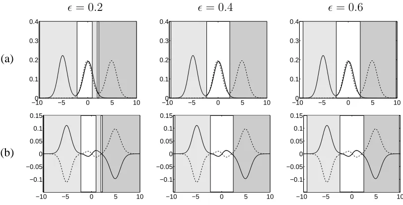
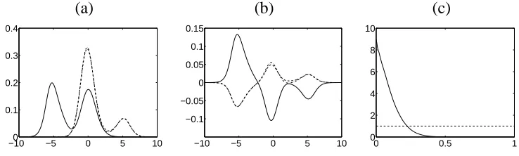
Figure 4:Example 1 (α1 =α2= 0.5): (a) Posterior predictive density for the two groups (Group 1 is solid

line and Group 2 is dashed line); (b) the differenceπ1 (solid line) andπ2(dashed line) indicating the area

where Group 1 has substantially more mass than Group 2 (light grey) and vice versa (dark grey).

Some results of fitting the model to data in the first example are shown in Figure 4. The

model estimates the densities well (shown in Row (a)). The graphs also show partitions of the

ǫ. The results are reasonably robust to the choice of ǫwith ǫ > 0.2 and they indicate that the distributions are similar between -2 and 2. This region seems slightly too small when

ǫ = 0.2, where the analysis reacts to the relatively small positive difference π1 in between

approximately 1 and 2. Row (b) shows the density of the differences π1 and π2. It is clear

from the definition that π2 = −π1 when we have two groups and this is illustrated in the

graphs which clearly show where the differences of the densities for the two groups are large.

a ρ

0 0.5 1

0 2 4 6 8 10

0 0.5 1

0 5 10 15

Figure 5: Example 1 (α1 = α2 = 0.5): Prior (dashed lines) and posterior (solid lines) densities of the

parameteraand the correlationρfor the NGG prior.

Figure 5 shows the posterior densities of the parameter a and the correlation ρ for the NGG prior. The data favour values of a smaller than 0.5. The posterior distribution of ρ

(calculated using the result of Theorem 1) is not very different from the prior suggesting that

the information in the data about correlation is not strong. The mass close to zero is in line

with the fact that the distributions that generated both groups are quite different.

(a) (b) (c)

−100 −5 0 5 10 0.1

0.2 0.3 0.4

−10 −5 0 5 10

−0.1 −0.05 0 0.05 0.1 0.15

0 0.5 1

0 2 4 6 8 10

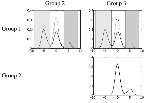
Figure 6: Example 2 (α1 = 0.5, α2 = 0.9): (a) Posterior predictive density for the three groups; (b)

differencesπ1,π2and π3 (Group 1 (π1) is solid line, Group 2 (π2) is dashed line and Group 3 (π3) is

Figure 6 shows results of fitting the model to the second example with three groups. The

density estimates clearly show the similarities between Groups 2 and 3 and the differences with

respect to Group 1. The plots ofπ1,π2and π3 in panel (b) clearly illustrate the main

differ-ences. Group 1 places more mass than Groups 2 and 3 on values less than -2 whereas Groups

2 and 3 place more mass than Group 1 on values larger than -2. The posterior distribution ofa

is very similar to that shown in Figure 5.

Group 2 Group 3

Group 1

−100 −5 0 5 10 0.1

0.2 0.3 0.4

−100 −5 0 5 10 0.1

0.2 0.3 0.4

Group 2

−100 −5 0 5 10 0.1

0.2 0.3 0.4

Figure 7:Example 2 (α1 = 0.5, α2= 0.9): Posterior mean density for the group in the row (solid line) and

column (dashed line) and comparison of the distributions with dark (light) grey areas indicating more mass

for the group in the column (row).

Figure 7 shows the results of making pairwise comparisons for the three groups, using

ǫ = 0.4. The results follow from the discussion of the differences between the distributions. In the comparisons between Group 1 and Groups 2 and 3 there are two separate regions with

important differences in the mass whereas the comparison between Group 2 and Group 3 shows

no differences between the distributions (as we would expect).

5.2

Survival analysis

Doss and Huffer (2003) discuss modelling interval censored data in survival analysis using the

DP as a prior for the distribution of the survival times. This application focuses on time to

cosmetic deterioration of the breast of women with Stage 1 breast cancer who have undergone

subjects in the radiation only group and 48 subjects in the combination group. The data has

been presented in Beadle et al. (1984). The indicatordg,j = 1if the j-th person in the g-th group suffers an event (in this case retraction of the breast) before the censoring timeTg,jand

dg,j = 0otherwise. Ifdg,j = 1 then the observation is an intervalAg,j in which the event occured. Doss and Huffer (2003) assign a Dirichlet process prior to the lifetime distribution

for each group separately. Since the actual survival times are missing (due to the interval

censoring), the posterior will then be a mixture of Dirichlet processes. Denoting the survival

time of individualjin groupgbyτg,j, we extend their approach to the model

I(τg,j ∈Ag,j) ifdg,j = 1or I(τg,j > Tg,j) ifdg,j = 0

τg,j ind.

∼ Gg

G1, G2, . . . , Gq∼CNGG(M, H, D;a, λ),

where H is an exponential distribution with mean 1/ξ. The parameter ξ is given a vague Gamma prior with shape parameter 0.1 and mean 1.

ǫ= 0_.2 _ǫ= 0_.4 _ǫ= 0_.6

(a)

0 50 100

0 0.2 0.4 0.6 0.8 1

months 0 50 100

0 0.2 0.4 0.6 0.8 1

months 0 50 100

0 0.2 0.4 0.6 0.8 1

months

(b)

0 50 100

−0.2 −0.15 −0.1 −0.05 0 0.05

months 0 50 100

−0.2 −0.15 −0.1 −0.05 0 0.05

months 0 50 100

−0.2 −0.15 −0.1 −0.05 0 0.05

months

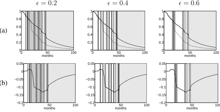
Figure 8: Survival analysis (combination group shown as dashed lines and radiation only group shown as solid lines): (a) the posterior mean survival functions for the two groups; (b) posterior mean forΠ1 where

the radiation only group is coded as Group 1 (Dark (light) grey areas indicate more mass for Group 2 (1)).

Figure 8 displays results of the analysis of the clinical trial data. Row (a) shows that the

survival function is similar for the two groups initially but the curves diverge around 16 months

the posterior mean of the difference between the survival functions for the groups. This also

indicates that the mass is similar until 16 months but then the difference quickly becomes large

until the survival functions converge again. The regions identified as similar change when

moving from ǫ = 0.4 to ǫ = 0.6 with the latter having fewer, larger and more connected regions. The results withǫ = 0.6more clearly highlight the larger differences in the survival functions, such as the sharp drop in the combination group around 16 months. Finally, for all

values ofǫthe radiation only group places more mass than the combination group in the region beyond 45 months.

a ρ

0 0.5 1

0 1 2 3 4

0 0.5 1

0 1 2 3 4 5

Figure 9: Survival analysis: Prior (dashed lines) and posterior (solid lines) densities of the parameteraand the correlationρ.

The posterior distributions of a and ρ are shown in Figure 9, which indicates that the value a = 0(the Dirichlet process case) is not well-supported by the data with a posterior median close to the Normalized Inverse-Gaussian process (wherea= 0.5), but with substantial posterior uncertainty. The posterior distribution of the correlation parameter ρindicates that the groups are different, but do share some common aspects.

5.3

Stochastic Frontier analysis

Stochastic frontier analysis is a popular method in econometrics for estimating the efficiency

of firms. We will consider an application to the efficiency of US hospitals using data previously

analyzed by Koop et al. (1997). It is assumed that all hospitals operate relative to a common

cost frontier, which represents the minimum cost of performing the functions of that hospitals

(including operations, patient care, etc.). It follows that inefficiency can be measured by how

far a hospital operates above the optimal cost level given by the frontier. The costs are observed

thej-th hospital in theg-th group at thet-th time point

Cg,j,t=α+xTg,j,tβ+ug,j+εg,j,t,

wherexg,j,t are variables used to define the frontier forj-th hospital in theg-th group at the

t-th time point,ug,j >0is the inefficiency for thej-th hospital in theg-th group andεi,j,tare mutually independent, measurement errors which will be assumed to be normally distributed

with mean 0 and varianceσ2. The model assumes that the efficiency of hospitals is fixed over the time period (a common assumption in the applied literature). The efficiency for thej-th hospital in theg-th group is defined to beexp{−ug,j}.

The main focus of this type of analysis is the distribution of the inefficiencies ug,j and estimation of the hospital efficienciesexp{−ug,j}. A Bayesian nonparametric analysis of the stochastic frontier model is described by Griffin and Steel (2004) who assume a DP prior for

the inefficiency distribution and apply their methods to the data analyzed here. The model used

here is

Cg,j,t ind.

∼ N(α+xT_g,j,tβ+ug,j, σ2)

ug,j ind.

∼ Gg

G1, G2, . . . , Gq∼CNGG(M, H, D;a, λ),

whereα,βandσ2_{are given the priors described by Griffin and Steel (2004) andHis an}

expo-nential distribution with mean1/ξ, whereξis given an exponential prior with mean−1/logr⋆_, so thatr⋆_{is the prior median efficiency. In this exampler}⋆_{is chosen to take the value 0.8.}

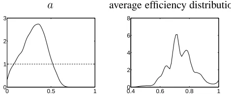
a average efficiency distribution

0 0.5 1

0 1 2 3

0.4 0.6 0.8 1

0 2 4 6 8

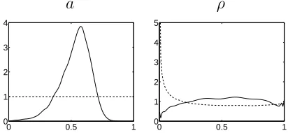
Figure 10: Stochastic Frontier Analysis: The posterior (solid line) and prior distributions (dashed line) of

aand the posterior mean of the average efficiency distribution with the NGG prior.

The data also include information about the type of hospital and include two factors: the

ownership status of the hospital (For-Profit, Non-Profit and Government) and a quality factor

in Koop et al. (1997). Figure 10 shows some posterior results of extending the model of Griffin

and Steel (2004) using the prior developed in this paper. The posterior distribution ofahas a mode at around 0.4. The posterior mean of the efficiency distribution averaged over all

hospital types has three internal modes at roughly 0.65, 0.7 and 0.8 and a further mode at 1,

which is quite in line with the results for the efficiency obtained in Griffin and Steel (2004)

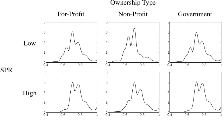
without using hospital type information. Figure 11 shows the posterior mean for the efficiency

Ownership Type

For-Profit Non-Profit Government

SPR

Low

0.4 0.6 0.8 1

0 2 4 6 8

0.4 0.6 0.8 1

0 2 4 6 8

0.4 0.6 0.8 1

0 2 4 6 8

High

0.4 0.6 0.8 1

0 2 4 6 8

0.4 0.6 0.8 1

0 2 4 6 8

0.4 0.6 0.8 1

0 2 4 6 8

Figure 11: Stochastic Frontier Analysis: The posterior mean of the efficiency distribution for each hospital type with a NGG prior.

distribution within each group. For comparison, an analysis using a product of DP is provided

by Griffin and Steel (2004). The prior developed in this paper leads to predictive distributions

which vary substantially less between groups, illustrating the model’s ability to effectively

borrow information. This is particularly important in this application where group sizes are

quite small, ranging from 20 to 141. All distributions are multi-modal with most distributions

having modes at roughly 0.7 and 0.8 (and at 1). However, the sizes of the modes differ between

the distributions.

Figure 12 shows the decomposition of the estimated distribution defined in (7). These

graphs more clearly show the differences and similarities between the distributions. Theπ’s show the effect of one factor averaging over the other factors. Hospitals with High SPR tend

have more mass at higher efficiency than Low SPR hospitals (suggesting that they tend to be

π’s

Low SPR High SPR

0.4 0.6 0.8 1

−1.5 −1 −0.5 0 0.5 1 1.5

0.4 0.6 0.8 1

−1.5 −1 −0.5 0 0.5 1 1.5

For-Profit Non-Profit Government

0.4 0.6 0.8 1

−1.5 −1 −0.5 0 0.5 1 1.5

0.4 0.6 0.8 1

−1.5 −1 −0.5 0 0.5 1 1.5

0.4 0.6 0.8 1

−1.5 −1 −0.5 0 0.5 1 1.5

γ’s

Ownership Type

For-Profit Non-Profit Government

SPR

Low

0.4 0.6 0.8 1

−0.5 0 0.5

0.4 0.6 0.8 1

−0.5 0 0.5

0.4 0.6 0.8 1

−0.5 0 0.5

High

0.4 0.6 0.8 1

−0.5 0 0.5

0.4 0.6 0.8 1

−0.5 0 0.5

0.4 0.6 0.8 1

−0.5 0 0.5

Figure 12: Stochastic Frontier Analysis: The posterior means of πi·, π·j and γi,j with NGG process marginals.

0.8. The For-Profit and Government hospitals have similar distributions and have more mass

at higher level efficiency than Non-Profit hospitals, again mostly involving shifts from regions

have particularly low mass at high levels of efficiency (around 0.8). Thus, the results clearly

indicate which factors (or combinations of factors) lead to distributions that place more mass

on higher levels of efficiency.

SPR Low High

Ownership NP Govt FP NP Govt

FP

0.5 1

0 5

0.5 1

0 5

0.5 1

0 5

0.5 1

0 5

0.5 1

0 5

Low NP

0.5 1

0 5

0.5 1

0 5

0.5 1

0 5

0.5 1

0 5

Govt

0.5 1

0 5

0.5 1

0 5

0.5 1

0 5

High FP

0.5 1

0 5

0.5 1

0 5

NP

0.5 1

0 5

Figure 13: Stochastic Frontier Analysis: Graphs of pairwise comparisons of efficiency distributions ac-cording to ownership type (FP=For-Profit, NP=Non-Profit, Govt=Government) and Staff-Patient Ratio. The

pairs are shown as the row (solid line) and column (dashed lines) with dark grey shading indicating higher

mass in the column and light grey shading indicating higher mass in the row.

Figure 13 shows pairwise comparisons of the distributions which identify regions where

the mass placed by the two corresponding distributions is substantially different, usingǫ= 0.4. These indicate that there is a lack of evidence of a difference between the For-Profit and

Gov-ernment hospitals at both quality levels (in line with their very similar π’s). There is also not much difference between the Non-Profit hospitals at high quality and the For-Profit and

Government hospital at Low quality (theπ’s for both factors more or less balance each other out). The other combinations of factors lead to clear results where we can identify regions of

the support where one distribution places more mass than the other and vice versa. Clearly,

the For-Profit and Government hospitals with high quality are the most efficient combinations,

re-strictive fully parametric model without interactions of Koop et al. (1997) leads to the very

different (and counterintuitive) conclusions that For-Profit status and high SPR both reduce

efficiencies.

6

Summary

This paper discusses a method for inferring differences between distributions associated with

different groups of observations. A Bayesian nonparametric approach is taken and we

intro-duce a novel form of priors, derived from Normalized Random Measures with Independent

Increments. The prior allows the inclusion of information about partial exchangeability and

so represents prior beliefs which could not be expressed using e.g. the Hierarchical Dirichlet

process. This allows effective borrowing of strength between distributions without assuming

exchangeability, and can easily and systematically accommodate widely varying levels of

com-plexity in terms of dependence. Efficient, exact inference is possible using a slice sampling

method, which extends the ideas of Griffin and Walker (2010). The prior is used with a new

graphical method to compare pairs of distributions. The common support of any two

distribu-tions is partitioned and each element of the partition is characterized by obtaining more mass

from either distribution or being allocated roughly similar mass by both distributions. This

is an effective way of understanding the difference between two distributions. In particular,

where the groups are defined by several covariates, we propose an informative ANOVA-type

decomposition of the differences.

We analyze applications in survival analysis and stochastic frontiers with small numbers of

observations, typical of real data applications in many fields. Despite this, the models perform

very well and lead to sensible results. Interestingly, in both applications, models with Dirichlet

process marginal processes are not well supported by the data and Normalized Generalized

Gamma marginals are favoured. The posterior distribution of a in the survival example is centred around0.5which corresponds to the Normalized Inverse-Gaussian process.

We believe the methodology proposed in this paper is highly flexible, yet widely applicable

to real data, and allows for quite informative inference on the (sources of the) differences

References

Beadle, G., S. Come, C. Henderson, B. Silver, and S. Hellman (1984). The effect of adjuvant

chemotherapy on the cosmetic results after primary radiation treatment for early stage breast

cancer. Inter. J. Rad. Oncol., Biol. Phys. 10, 2131–2137.

Brix, A. (1999). Generalized gamma measures and shot-noise Cox processes. Adv. in Appl.

Probab. 31, 929–953.

De Iorio, M., P. M¨uller, G. L. Rosner, and S. N. MacEachern (2004). An ANOVA Model for

Dependent Random Measures. J. Amer. Statist. Assoc. 99, 205–215.

Doss, H. and F. W. Huffer (2003). Monte Carlo methods for Bayesian analysis of survival data

using mixtures of Dirichlet process prior. J. Comput. Graph. Statist. 12, 282–307.

Dunson, D. B., Y. Xue, and L. Carin (2008). The matrix stick breaking process: Flexible Bayes

meta analysis. J. Amer. Statist. Assoc. 103, 317–327.

Ferguson, T. S. (1973). A Bayesian analysis of some nonparametric problems. Ann. Statist. 1,

209–230.

Griffin, J. E. (2009). The Ornstein-Uhlenbeck Dirichlet Process and other time-varying

non-parametric priors. Technical report, University of Warwick.

Griffin, J. E. and P. J. Brown (2010). Inference with Normal-Gamma prior distributions in

regression problems. Bayesian Analysis 5, 171–188.

Griffin, J. E. and M. F. J. Steel (2004). Semiparametric Bayesian inference for stochastic

frontier models. J. Econometrics 123, 121–152.

Griffin, J. E. and S. G. Walker (2010). Posterior simulation of Normalised Random Measure

mixtures. J. Comput. Graph. Statist., forthcoming.

James, L. F., A. Lijoi, and I. Pr¨unster (2009). Posterior analysis for normalized random

mea-sures with independent increments. Scand. J. Statist. 36, 76–97.

Kalli, M., J. E. Griffin, and S. G. Walker (2011). Slice sampling mixture models. Statistics

Kingman, J. (1975). Random discrete distributions. J. R. Stat. Soc. Ser. B 37, 1–22 (with

discussion).

Kolossiatis, M., J. E. Griffin, and M. F. J. Steel (2010). On Bayesian nonparametric modelling

of two correlated distributions. Technical report, University of Warwick.

Koop, G., J. Osiewalski, and M. F. J. Steel (1997). Bayesian efficiency analysis through

indi-vidual effects: Hospital cost frontiers. J. Econometrics 76, 77–105.

Lijoi, A., R. H. Mena, and I. Pr¨unster (2005). Hierarchical mixture modeling with normalized

inverse-Gaussian priors. J. Amer. Statist. Assoc. 100, 1278–1291.

Lijoi, A., R. H. Mena, and I. Pr¨unster (2007). Controlling the reinforcement in Bayesian

non-parametric mixture models. J. R. Stat. Soc. Ser. B 69, 715–740.

M ¨uller, P., F. Quintana, and G. Rosner (2004). A method for combining inference across

related nonparametric Bayesian models. J. R. Stat. Soc. Ser. B 66, 735–749.

Rodriguez, A., D. Dunson, and J. Taylor (2009). Bayesian hierarchically weighted finite

mix-ture models for samples of distributions. Biostatistics 10, 155–171.

Scott, J. G. and N. G. Polson (2011). Shrink globally, act locally: Sparse Bayesian

regulariza-tion and predicregulariza-tion. In Bayesian Statistics 9. Oxford University Press.

Teh, Y. W., M. I. Jordan, M. J. Beal, and D. M. Blei (2006). Hierarchical Dirichlet processes.

J. Amer. Statist. Assoc. 101, 1566–1581.

A

Proof of Theorem 1

We know that E[G1(B)] =E[G2(B)] =H(B). To calculate the covariance, we need

E[G1(B)G2(B)] =E "

˜

G1(B)

˜

G1(Ω)

˜

G2(B)

˜

G2(Ω) #

=E





˜

G⋆

1(B) + ˜G⋆2(B) G˜⋆1(B) + ˜G⋆3(B)

˜

G⋆

1(Ω) + ˜G⋆2(Ω) G˜⋆1(Ω) + ˜G⋆3(Ω)





=

Z ∞

0 Z ∞

0

where

γ(v1, v2) =

˜

G⋆₁(B) + ˜G⋆₂(B) G˜⋆₁(B) + ˜G⋆₃(B)

×expn−v1

˜

G⋆₁(Ω) + ˜G⋆₂(Ω)−v2

˜

G⋆₁(Ω) + ˜G⋆₃(Ω)o =G˜⋆₁(B)2+ ˜G⋆₁(B) ˜G⋆₃(B) + ˜G⋆₂(B) ˜G⋆₁(B) + ˜G⋆₂(B) ˜G⋆₃(B)

×expn−(v1+v2) ˜G⋆1(Ω)−v1G˜⋆2(Ω)−v2G˜⋆3(Ω) o

The independence of the underlying processesG˜⋆

1,G˜⋆2 andG˜⋆3 and the independence of L´evy

processes on disjoint sets gives

E[γ(v1, v2)] =E

h

˜

G⋆₁(B)2expn−(v1+v2) ˜G⋆₁(B)oiE

h

expn−(v1+v2) ˜G⋆₁(Bc)oiE

h

expn−v1G˜⋆₂(Ω)oi

×E

h

expn−v2G˜⋆3(Ω) oi

+E

h

˜

G⋆₁(B) expn−(v1+v2) ˜G⋆1(B) oi

E

h

˜

G⋆₃(B) expn−v2G˜⋆3(B) oi

×E

h

expn−(v1+v2) ˜G⋆₁(Bc)oiE

h

expn−v1G˜⋆₂(Ω)oiE

h

expn−v2G˜⋆₃(Bc)oi +E

h

˜

G⋆₂(B) expn−v1G˜⋆2(B) oi

E

h

˜

G⋆₁(B) expn−(v1+v2) ˜G⋆1(B) oi

E

h

expn−(v1+v2) ˜G⋆1(Bc) oi

×E

h

expn−v1G˜⋆2(Bc) oi

E

h

expn−v2G˜⋆3(Ω) oi

+E

h

˜

G⋆₂(B) expn−v1G˜⋆2(B) oi

×EhG˜⋆₃(B) expn−v2G˜⋆3(B) oi

Ehexpn−(v1+v2) ˜G⋆1(Ω) oi

Ehexpn−v1G˜⋆2(Bc) oi

×E

h

expn−v2G˜⋆3(Bc) oi

The definition ofLη(v)implies that E[exp{−vG˜⋆

k(B)}] = exp{−H(B)MkLη(v)} and then

EhG˜⋆_k(B) exp{−vG˜⋆_k(B)}i=−E

d

dv exp{−vG˜

⋆ k(B)}

=− d

dvE h

exp{−vG˜⋆_k(B)}i

=− d

dvexp{−H(B)MkLη(v)}=H(B)MkL

′

η(v) exp{−H(B)MkLη(v)}

E

˜

G⋆_k(B)2exp{−vG˜⋆_k(B)}

=E

d

dv2exp{−vG˜

⋆ k(B)}

= d

dv2E h

exp{−vG˜⋆_k(B)}i

=hH(B)2M_k2 L′_η(v)2

−H(B)MkL′′η(v)

i

It follows that

E[γ(v1, v2)]

=hH(B)2M₁2 L′_η(v1+v2) 2

−H(B)M1L′′η(v1+v2) i

exp{−H(B)M1Lη(v1+v2)}

×exp{−(1−H(B))M1Lη(v1+v2)}exp{−M2Lη(v1)}exp{−M3Lη(v2)}

+H(B)M1L′η(v1+v2) exp{−H(B)M1Lη(v1+v2)}H(B)M3L′η(v2) exp{−H(B)M3Lη(v2)}

×exp{−(1−H(B))M1Lη(v1+v2)}exp{−M2Lη(v1)}exp{−(1−H(B))M3Lη(v2)}

+H(B)M2L′η(v1) exp{−H(B)M2Lη(v1)}H(B)M1L′η(v1+v2) exp{−H(B)M1Lη(v1+v2)}

×exp{−(1−H(B))M1Lη(v1+v2)}exp{−(1−H(B))M2Lη(v1)}exp{−M3Lη(v2)}

+H(B)M2L′η(v1) exp{−H(B)M2Lη(v1)}H(B)M3L′η(v2) exp{−H(B)M3Lη(v2)}

×exp{−M1Lη(v1+v2)}exp{−(1−H(B))M2Lη(v1)}exp{−(1−H(B))M3Lη(v2)}

=

H(B)2 M2L′η(v1) +M1L′η(v1+v2)

M3L′η(v2) +M1L′η(v1+v2)

−H(B)M1L′′η(v1+v2)

×exp{−M1Lη(v1+v2)}exp{−M2Lη(v1)}exp{−M3Lη(v2)}.

Then

Cov(G1(B), G2(B)) =H(B)2

Z ∞

0 Z ∞

0

αγ dv1dv2−1

−H(B)

Z ∞

0 Z ∞

0

βγ dv1dv2

where

α= M2L′η(v1) +M1L′η(v1+v2)

M3L′η(v2) +M1L′η(v1+v2)

,

β=M1L′′η(v1+v2) and

γ = exp{−M1Lη(v1+v2)−M2Lη(v1)−M3Lη(v2)}.

The result follows from the fact that

Z ∞

0 Z ∞

0

αγdv1dv2 = 1+ Z ∞

0 Z ∞

0