Computational Studies of Pressure Distribution around a 5:1 Rectangular Section
in Turbulent Flow
Dinh Tung Nguyen1, David Hargreaves1, John Owen1 1
Department of Civil Engineering, Faculty of Engineering, University of Nottingham, Nottingham, UK Email: [email protected], [email protected], [email protected]
ABSTRACT: This paper presents a numerical method based on a LES approach to modelling the unsteady flow around and the vortex-induced vibration (VIV) of a 5:1 rectangular cylinder in the smooth and turbulent flow. A fluid-structure interaction algorithm was also developed to model the aerodynamic behaviour of a half of the bridge deck in the bending and torsional modes. Results from the static and heaving simulations have validated the accuracy of the proposed computational method and revealed the important role of the motion-induced vortex during the lock-in and its interaction with the von Karman vortex. By introducing the bending motion on the bridge deck, some preliminary results of the bending simulation have indicated some distinct features including the variation of the surface pressure and the separation bubble in the spanwise direction which could promote the spanwise flow. The relative strength between the motion-induced vortex and the von Karman vortex was observed to vary across the spanwise length of the bridge deck, largely influencing the response of the bridge deck in the lock-in. The project will go on to investigate these features together with the surface pressure distribution and the pressure coherence and correlation structure in order to offer a quantitative explanation on the turbulence-induced effect on the VIV and torsional flutter of a 5:1 rectangular cylinder.
KEY WORDS: Bridge Aerodynamics; 5:1 Ratio; Rectangular Section; Pressure Distribution; CFD; Large Eddy Simulation; Turbulent Flow; VIV.
1 INTRODUCTION
The rectangular cylinder has been considered as a simplified geometry of many structures in the built environment including the main section of a suspension bridge. It has been studied intensively among researchers to uncover important insights into the aeroelastic and aerodynamic responses of the bridge deck and to verify new methods of wind loading analysis. Different from the circular cylinder, the rectangular cylinder is characterised by the permanent separation point at the leading edge causing two unstable shear layers along surfaces of the body. Their properties are largely controlled by the aspect ratio (i.e. the ratio between the width and the depth of the cross section) and the Reynolds number [1][2][3][4]. More importantly, the interaction between the leading-edge shear layer and the von Karman vortex shed from trailing edge governs the aerodynamic responses [5][6]. Therefore, the rectangular cylinder is very prone to VIV, torsional flutter and classical flutter.
In this paper, the 5:1 rectangular cylinder is selected as a case study since it is considered as a basic bridge deck geometry. Previous wind tunnel experiments revealed that this section is classified into the category of intermittent reattachment flow where the aforementioned shear layer forms two separation bubbles which reattach at points very close the trailing edge [7][8]. This feature highlights the unsteadiness of the flow field around the cylinder. In addition, the variation of the Reynolds number was found to have a suppression effect on these bubbles. By promoting the Reynolds stress and turbulent entrainment, an increase in the Reynolds number leads to a reduction in the length of the separation bubble and a quick recovery of surface pressure [9]. The upstream turbulence was also found to produce similar effects on the separation bubble but to a higher degree. The turbulent wind significantly amplifies the suction peak and moves it upstream yielding a smaller separation bubble, an increased longitudinal curvature of the shear layer near the leading edge and earlier pressure recovery [10]. Further papers pointed out that the turbulence-induced effects on the pressure distribution around a 5:1 rectangular cylinder, including a decrease in the pressure correlation and coherent structures [11][12]. Later, the authors in [13] suggested that this alteration of the surface pressure is responsible for the damping effects of turbulence on flutter which was previously observed in [14]. Another review in [15] showed that increased turbulence produces a stabilising effect on the VIV of a 5:1 rectangular cylinder; however, a comprehensive explanation of the mechanism is still to be found.
were self-developed by authors [16][17]. Due the complexity of the problem and the limitation of computational power, the spatial discretisation of the computational grid was coarse relative to current standards and the simulation was restricted to model the flow field around a 2D static cylinder only. Later, a lot of efforts have been devoted to the development of standard approaches to numerically solve the Navier-Stoke equations. Among of them, the two-equation Unsteady Reynolds-Averaged Navier-Stokes (URANS) models are the most commonly used due to their simplicity and self-completeness. There are the k-ε and k-ω turbulence models with different versions; the former is less preferable in the application of the bridge aeroelasticity because it does not allow a direct integration to the wall through the boundary layer and over-predicts the turbulence kinetic energy at impingement on the wall [18]. On the other hand, the latter helps resolve these issues but its sensitivity to the free-stream turbulence was remarked in [19]. A solution therefore was proposed in [20] by using a blending function to assign the ω to the near wall region and the ε in the remaining computational domain, which is called the Shear-stress-transport (SST) k-ω model. The suitability of this model was tested in [21] through a series of numerical examples of a dynamic cylinders where the flutter derivatives were used to quantify its aeroelasticity. The authors in [21] were able to estimate all 18 flutter derivatives reasonably agreeing with experimental results and reflecting the effect of the free stream turbulence. A 3D simulation was also performed and yielded results identical to the 2D simulation. This fact emphasises that an assumption of the isotropic turbulence is embedded in the URANS model; the 3D features of the flow field around the cylinder and especially in the wake therefore is not accurately captured.
With the development in computational technologies, 3D simulations which use the Large Eddy Simulation (LES) model have become more available. The basic idea of the LES model is that a spatial filtering function with a prescribed filtering length scale is used to separate the large eddies from the small ones. Most Computational Fluid Dynamics (CFD) codes use an implicit filtering function where the cell size is effectively the filtering length scale. The LES approach directly resolves the large eddies while the small eddies are modelled by the use of a sub-grid scale model which simulates the transportation of momentum and energy between eddies of different sizes. Currently the LES approach is mostly concentrated on investigating the complex flow field and surface pressure distribution around a static rectangular cylinder [22][23]. Their numerical results were in a good agreement with the wind tunnel tests regarding the coherent structure of the surface pressure and the effect of the afterbody length on the separation and reattachment characteristics of the flow. The LES approach was also coupled with a structural solver to model the fluid-structure interaction (FSI) of a 3D elastically supported rectangular cylinder at a low Reynolds number flow [24]. Despite differences in a comparison against the wind tunnel results, it highlighted the suitability of the LES model to capture the inherent unsteadiness in FSI problems. Also, the LES approach is capable to maintain the turbulence structure in the wake region in contrast to the over-dissipation of the URANS turbulence models. Later, the authors in [25] were able to apply this method to predict the effect of the free-stream turbulence on the aerodynamic behaviour of a static and elastically mounted 5:1 rectangular cylinder. Although the spanwise discretisation was coarse, the preliminary sets of results revealed the turbulence-induced effects as observed in wind tunnel experiments. The use of the LES approach is still limited in industrial application due to its computationally expensive near-wall treatments. In addition, as shown in [26], results of 3D LES simulations in the application of the bridge aeroelasticity are very susceptible to the level of discretisation in the spanwise direction.
In this project, utilising the High Performance Computer at the University of Nottingham, the aforementioned coupling approach between the LES model and the FSI solver is applied to simulate the aerodynamic and aeroelastic responses of a static and elastically supported 3D sectional rectangular cylinder of the 5:1 aspect ratio in the smooth and turbulent flow. In addition, a mode shape is embedded into the FSI solver in order to model responses of a half of the bridge deck. The comparison between these models will offer an explanatory discussion of emerging flow features in the spanwise direction and the turbulence-induced effect on the pressure distribution and aeroelastic responses.
2 DEFINITION OF THE FLUID PROBLEM
The unsteady flow around the rectangular cylinder is governed by the incompressible Navier-Stokes equations which are
0
i i
x
u
, (1)
j i j
i j
i j i
x
u
x
x
p
u
u
x
u
t
, (2)0
t
u
i, (3)
i j j i SGS j i j i j ix
u
x
u
x
x
p
u
u
x
u
t
. (4)Here, 𝑢̅ and 𝑝̅ are the filtered velocity and pressure. μSGS is the sub-grid scale (SGS) viscosity and it is modelled by the used of the conventional Smagorinsky SGS model. However, to avoid the overestimation of the Smagorinsky constant and to account for the effects of convection, diffusion, production and destruction on the SGS velocity scale [27], an additional transportation equation is embedded to determine the distribution of the kinetic energy of the SGS eddies, kSGS
32.
2
SGS ij ij SGS j SGS SGS j j SGS j SGSk
C
S
S
x
k
x
u
k
x
k
t
, (5)where μSGS = ρCSGS(kSGS)1/2, the constants are set equal to Cε = 1.05 and CSGS = 0.07 and is the characteristic length scale of the filter which is related to the mesh size and defined as the cubic root of the cell volume. In addition, to remove the over-dissipation of kinetic energy in the near-wall region, a filtered width damped according to the van Driest approach is introduced as
A ye
y
C
k
1
,
min
, (6)where k = 0.4187 is the von Karman constant, C = 0.158 and A+ = 26 are the van Driest constants and y and y+ is the normal
distance and non-dimensional distance to the wall. In other words, in the near-wall region, the length scale of the filter is not essentially related to the mesh cell size; the minimum value between and the one obtained from the damping function in Equation 6 is locally adopted.
3 FLUID-STRUCTURE INTERACTION
The FSI problem in this project is modelled by the use of the Arbitrary Lagrangian-Eulerian (ALE) algorithm which helps eliminate the disadvantages of the conventional Lagrangian and Eulerian methods in modelling problems involving excessive distortions of continuum (either the fluid or structure)[28]. The ALE algorithm however introduces the convection effect due to the motion of the grids node which must be embedded into Equations 3 and 4 as
0
u
u
t
i , (7)
i j j i SGS j i i j j ix
u
x
u
x
x
p
u
u
u
x
u
t
, (8)where 𝑢̂ is the velocity of the grid nodes. 3.1 Structural solver
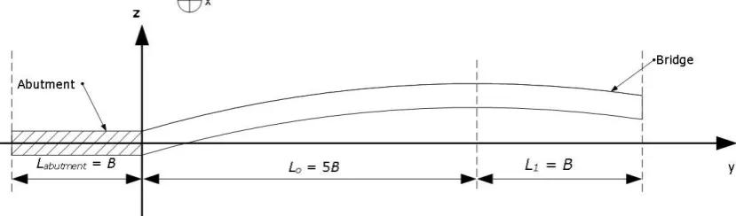
The single-degree-of-freedom equation of motion of the bridge is expressed in the spatial and temporal domain with respect the coordinate system shown in Figure 1 as
),
,
(
)
,
(
)
,
(
)
,
(
y
t
c
Z
y
t
kZ
y
t
F
y
t
Z
m
(9)method is used to solve Equation 9. Here only the first mode shape is taken into account which is n(y) = osin[/(2Lo) y]; the modal amplitude o can be prescribed such that the generalised mass is equal to 1. Equation 9 is then transformed into
),
(
)
(
)
(
2
)
(
t
z
t
2z
t
f
t
z
n
n
(10)where f(t) is the generalised force acting on the bridge, and n is the damping ratio and the natural frequency of the first bending mode respectively. The first-order backward Euler method is applied to discretise and numerically solve Equation 10
),
(
)
(
2
)
(
)
(
t
n 1f
t
n nz
t
n n2z
t
nz
(11),
)
(
)
(
)
(
t
1z
t
z
t
1t
z
n
n
n
(12).
)
(
)
(
)
(
t
1z
t
z
t
1t
z
n
n
n
(13)Here, t is the time-step size, f(tn) is the generalised force acting on the bridge at the time step tn, 𝑧(𝑡𝑛), 𝑧̇(𝑡𝑛) and 𝑧̈(𝑡𝑛) are the generalised displacement, velocity and acceleration of the bridge deck at the time step tn and 𝑧(𝑡𝑛+1), 𝑧̇(𝑡𝑛+1) and 𝑧̈(𝑡𝑛+1) are the generalised displacement, velocity and acceleration of the bridge deck at the time step tn+1. This proposed algorithm can also be used to simulate the first torsional modal response.
3.2 Dynamic mesh algorithm
Together with the use of the ALE algorithm to model the FSI problem, a dynamic mesh algorithm must be prescribed and implemented to accommodate the deformation of the bridge deck. The computational domain can be divided into 9 separated blocks as shown in Figure 2. Blocks 1 and 3 are rigid where all grid nodes are effectively fixed relative to the bridge. The other blocks are grouped into a buffer zone where cells are allowed to deform to facilitate the displacement of the bridge.
The algorithm to displace the grid nodes in the buffer zone is based on the linear spring algorithm proposed in [29]. Effectively, the edges of the mesh are modelled to behave like linear springs connecting mesh vertices; the stiffness of the springs is inversely proportional to the length of the edges. In addition, the grid nodes on the outer boundaries of the mesh are held fixed whereas the ones on the structures are fixed relatively to the moving boundary. Some disadvantages of the linear spring algorithm have been mentioned in the later papers; however, via some preliminary test, this approach is appropriate taking into account the fact that the displacement of the bridge deck is small compared to the cell size in the buffer zone. 3.3 Coupling schemes
In this project, the conventional serial staggered algorithm is applied to model the coupling between the fluid, structure and dynamic mesh. This method is illustrated in Figure 3; there are 4 steps involving which are:
1. Update the fluid mesh based on the new structural boundary,
2. Solve the Navier-Stokes equations and advance the fluid domain with the new boundary conditions, 3. Use the new fluid solutions to calculate the new loads acting on the structure,
4. Solve the structural equation with the new loads and advance the structural domain.
[image:4.595.94.509.603.725.2]A number of reviews have pointed out the loose coupling problem of this algorithm which is responsible for its instability and the need of a small time-step size. Some improvements have been proposed but they can be overshadowed by an increase in the computational power. In fact, the authors in [30] have pointed out, if the numerical schemes solving the fluid governing equations are second-order, the stability of this scheme can be preserved without complicating the computational implementation and increasing the computational cost.
Figure 2. Illustration of 9 different blocks in the computational domain.
Figure 3. Conventional serial staggered algorithm.
4 APPLICATION
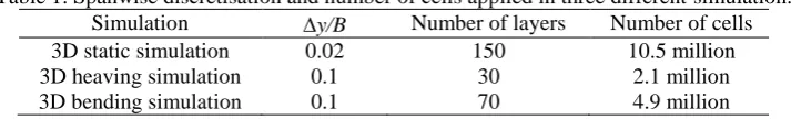
The computational studies were calculated using the open-source Computational Fluid Dynamics software OpenFOAM v2.2.2. The computational domain and boundary conditions are shown inFigure 4. A zero gradient condition for velocity and constant value of zero pressure were imposed on the outlet. As for the inlet, a non-zero x-component wind speed and a zero gradient condition for pressure were specified to simulate smooth flow. The turbulent field in this study was generated using the third-party software package LEMOS v.2.2.2, produced by researchers in Rostock University. This method uses an autocorrelation function defined using the prescribed turbulence length scale to compute the velocity distribution at random points on the inlet. The Lund’s transformation is then implemented to correct the correlation as described by the distribution of Reynolds stresses [31]. In addition, the movingWallVelocity boundary condition was specified on the surface of the bridge to accurately capture a zero normal-to-wall velocity component particularly in dynamic simulations.
The length of the domain (in the y direction) was L = 3B for the 3D sectional model which was satisfied the requirement proposed by [32] and able to capture the 3D nature of the flow. On the other hand, the flexible model utilised L = 7B to facilitate some deflection of the bridge deck. The fluid computational domain was discretised using a 3D hybrid hexahedral grid, where the grid was hybrid in the x-z plane (Figure 5) and structured in the y direction. A 6-layer structured grid was imposed around the bridge deck where the thickness of cells next to the model was z/B = 210-3 and grew by the ratio of 1.2. The constant discretisation in the along-wind direction was x/B = 2z/B. The unstructured hexahedral grid was used for the remaining part of the x-z plane. The 3D grid was constructed by projecting the 2D grid along the y direction. Due to the current limitation of the computational energy, different values of the spanwise discretisation between the static and dynamic simulations were applied (Table 1); the 3D sectional model was used to perform the 3D static and heaving simulations while the 3D bending simulations were carried out on the 3D flexible model.
The pressure-velocity coupling was achieved by means of the PIMPLE algorithm, which is a merged PISO-SIMPLE solver. It performs two PISO loops which leads to better coupling between pressure and velocity and allows bigger time-steps and Courant numbers. The convection terms were discretised by the use of the limited linear; the second-order central differencing scheme was applied to the diffusion terms. The non-dimensional time-step t*=tU/B (t is the time-step and U is the upstream wind speed) was set equal to 210-3. Simulations were extended over 80 non-dimensional time-steps to obtain converged statistics and data in the further 120 non-dimensional time-steps was used to perform analysis.
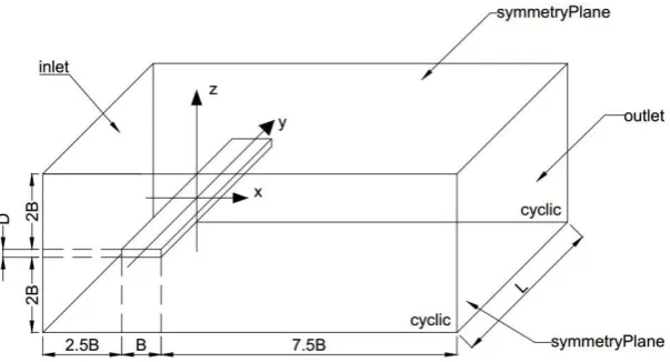
Table 1. Spanwise discretisation and number of cells applied in three different simulation. Simulation y/B Number of layers Number of cells
3D static simulation 0.02 150 10.5 million
3D heaving simulation 0.1 30 2.1 million
[image:5.595.120.477.687.741.2]Figure 4. Computational domain and boundary conditions
Figure 5. The computational grid in the x-z plane for the entire domain (a) and zoomed-in around the leading edge (b).
Figure 6. Locations of pressure measurement points (dimensions are normalised by the depth, D).
4.1 Static simulations
The OpenFOAM’s solver pimpleFoam was used to simulate the flow around the 3D static sectional model. The model was tested at 3 different wind speeds, 1, 2 and 4 ms-1. At each wind speed, the surface pressure data was extracted at points shown in Figure 6. Each pressure sampling line included 19 measurement points separated by 0.04 m. There were 4 additional pressure sampling points located near the leading edge (red dots) and near the trailing edges (black dots) respectively. Simulations were repeated in the smooth flow and in three levels of incident turbulence.
4.2 Dynamic simulations
[image:6.595.128.460.433.542.2]As for the 3D bending simulation, a mode shape n(y) with the modal amplitude o = 0.363 is used. Due the relative displacement between the high-y and low-y patches, the symmetryPlane boundary condition must be applied on them instead of the cyclic condition as in the simulations of the 3D sectional model. With the length of the domain specified in this study, the effect due to the symmetryPlane boundary condition could be minimised and half of the first bending and torsional modes were simulated. The mass per unit length 𝑚̅ is set to be 4.73 kgm-1, which was equivalent to the 3D sectional model. A similar damping ratio = 0.01 and natural frequency of the bending mode fnb = 1.2 Hz were applied. The surface pressure distribution was measured to identify the effect of flow in the spanwise direction on the pressure distribution and aerodynamic behaviour of the bridge deck. Dynamic simulations were also conducted in the smooth flow and in three levels of incident turbulence. 5 RESULTS AND DISCUSSION
5.1 Static simulations
Selected integral parameters at three different Reynolds numbers are summarised in Table 2. 𝐶𝐷 and 𝐶𝐿 are the time-averaged drag and lift coefficients respectively (using B as the characteristic length scale); 𝐶𝐿′ is the standard deviation of the time variation of the lift coefficient; St is the Strouhal number defined from the spectral analysis of the lift coefficient. Except for 𝐶𝐿, the comparison showed a good agreement between the current numerical studies and wind tunnel tests. There was approximately a 30% difference in 𝐶𝐿′ at the Reynolds number of 27000 which could be due to the short length of lift coefficient time series. The numerical studies predicted negative values of 𝐶𝐿, which was also reported on other LES simulations [26]. An isosurface of the Q-criteria value, Q = 0.1 s-1, of the flow field is shown in Figure 7, which illustrates that the scale of vortices in the bottom half of the wake was bigger than that in the top half. This difference implied larger suction on the bottom surface of the bridge deck, resulting in the negative lift force. One possible reason for this discrepancy is the slight asymmetry between the top and bottom halves of the unstructured grid regarding the cell density and cell size, which may lead to the fact that the flow is resolved differently on either side of the bridge deck.
[image:7.595.114.493.435.636.2]The surface pressure distribution at the Reynolds number of 6700 was analysed and compared against selected wind tunnel tests. In Figure 8, the pressure correlation from the current studies shows a reasonable agreement with the wind tunnel results, especially at the downstream location; the difference could be partly due to the effects of the Reynolds number. Both sets of results showed the pressure was more correlated at the upstream position, i.e. inside the separation bubble, compared to the downstream position, i.e. around the reattachment points. It implied the flow field inside the separation bubble was dominated by 2D flow features due the separation point at the leading edge; on the other hand, the flow field was more intermittent where the reattachment occurred.
Table 2. A comparison of selected integral parameters obtained from this numerical study and wind tunnel tests.
Re St 𝐶𝐷 𝐶𝐿 𝐶𝐿′
Current studies
6700 0.608 0.241 -0.056 0.081
13000 0.600 0.206 -0.059 0.075
27000 0.609 0.206 -0.063 0.059
[11] 6000 – 40000 0.555 0.242 0 0.08
Figure 7. Isosurfaces of Q = 0.1 s-1 around the bridge deck and in the wake region (Re = 6700).
Figure 8. Spanwise correlation of pressure coefficients. Wind tunnel results from [33] at Re = 63600.
Figure 9. Spanwise coherence of pressure. The top row corresponds to the upstream locations (x/D = 1.6) while the other corresponds to the downstream locations (x/D = 1.6). Wind tunnel results from [12] at Re = 40000.
The good agreement of integral coefficient, flow structure and surface pressure distribution between the current studies and selected wind tunnel studies highlights the appropriateness and accuracy of the proposed numerical approach in modelling the unsteady flow around the 5:1 rectangular cylinder. The use of the unstructured grid, however, could be an issue since the symmetry of the computational domain was not completely satisfied, which might cause the asymmetric flow structure in the wake and a negative lift force.
5.2 Heaving simulations
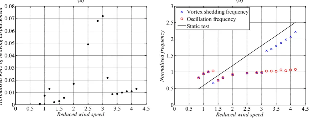
The response of the 3D sectional model in the heaving mode is characterised by two peaks as can be seen in Figure 10(a). The first peak occurred at the reduced wind speed Ur = 0.83; the magnitude of this peak was a lot smaller than the second one which was observed at Ur = 1.67. These two peaks correspond to the lock-in where the vortex shedding frequency is locked into the natural frequency of the structure as shown in Figure 10(b). Here the root-mean-squared displacement was normalised by the depth D of the section; frequency values are normalised by the natural frequency fnh of the heaving mode of the structure.
It was noticed the onset reduced velocity of the first peak was equal to a half of that of the second peak; this relationship was discussed in [5] and related to a difference in the flow field around the section which is clearly illustrated via the contour plots of
0 1 2 3 4 5 6 7 8
0 0.2 0.4 0.6 0.8 1 y/D Co rr el at io n of p res su re co ef fi ci en ts
(a) x/D = -1.6
0 1 2 3 4 5 6 7 8
0 0.2 0.4 0.6 0.8 1 y/D Co rr el at io n of p res su re co ef fi ci en ts
(b) x/D = 1.6
Wind tunnel studies Current studies
0 0.2 0.4 0.6 0.8 1 1.2 0 0.2 0.4 0.6 0.8 1 Co he re nc e fB/U (a) y/D = 0.42
0 0.2 0.4 0.6 0.8 1 1.2 0
0.2 0.4 0.6 0.8
1 (b) y/D = 1.00
fB/U Co he re nc e
0 0.2 0.4 0.6 0.8 1 1.2 0
0.2 0.4 0.6 0.8
1 (c) y/D = 2.08
fB/U Co he re nc e
0 0.2 0.4 0.6 0.8 1 1.2 0
0.2 0.4 0.6 0.8
1 (d) y/D = 0.42
fB/U Co he re nc e
0 0.2 0.4 0.6 0.8 1 1.2 0
0.2 0.4 0.6 0.8
1 (e) y/D = 1.00
Co
he
re
nc
e
fB/U 0 0.2 0.4 0.6 0.8 1 1.2
0 0.2 0.4 0.6 0.8
1 (f) y/D =2.08
[image:8.595.44.558.317.563.2]Q-criteria value, Q = 0.1 ms-1, on the mid-span plane during the lock-in. At Ur = 1.17 when the section reached the maximum displacement in the first peak, Figure 11 showed there were two vortices alternatively being formed on either side of the section. Their arrival at the trailing edge was synchronised with the motion of the section. On the other hand, when the section was at the maximum displacement in the second peak, there was only one vortex alternatively shed from the leading edge as shown in Figure 12.
In Figure 10(b), the shedding frequency of the von Karman vortex obtained from the static simulation was also included. It showed the vortex shedding frequency outside the lock-in did not well agree with the prediction obtained from the static simulation, which could be due to different levels of spanwise dicretisation. The LES approach with an implicit filtering method is known to be very susceptible to the geometry of cells in the computational domain. The use of the coarse spanwise discretisation could imply large SGS viscosity and a distortion of the geometry of eddies.
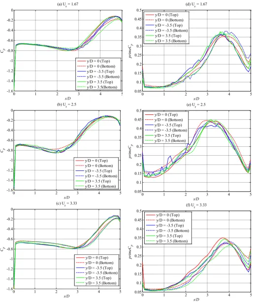
The surface pressure distribution were measured on the top and bottom surfaces of the section at three different spanwise positions which were the mid-span position y/D = 0 and on either side of the mid span y/D = 1.15. The results obtained during the lock-in were compared against those before and after the lock-in to reveal the variation of the flow field around the section. Implied from Figure 13, during the lock-in, the separation bubble was seen to be shorter leading to quicker recovery of pressure near the trailing edge. The shear layer reattached to the surface at the point of s/D = 2.5 when the section is in the lock-in; outside the lock-in, the reattachment point was found to be around s/D = 3.25. The reattachment point was estimated as the midpoint between the points corresponding to the minimum of 𝐶𝑃 and the maximum of 𝐶𝑃′. Also, in the lock-in, the motion of the section amplified the strength of the separation bubble which can be seen via an increase in the suction peak and in fluctuation of the pressure around the reattachment point. It is also noticed that outside the lock-in i.e. when the displacement of the section was small, there was a slight difference in pressure distribution between the top and bottom surfaces which could be resulted from an asymmetry mesh density between the top and bottom halves of the domain as being discussed in Section 5.1.
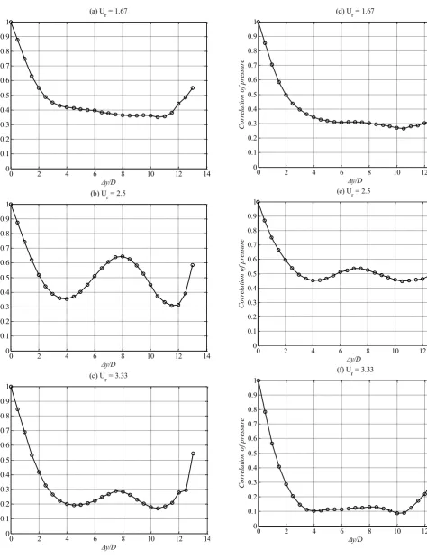
[image:9.595.50.555.447.639.2]The pressure correlation was calculated from the pressure data obtained from two arrays of 27 sampling points separated by a gap of 0.05 m. One array was located at x/H = 0.09 from the leading edge while the other was at x/H = 0.41. Despite the effect of the cyclicboundary condition which led to an increase in the pressure correlation from y/H = 10, the pressure correlation curves approach to a non-zero asymptote, which implies there was a portion of flow that was perfectly correlated in the spanwise direction (Figure 14). Overall, the fully correlated portion was lower near the trailing edge, highlighting the unsteadiness of the flow around the reattachment point. During the lock-in, the pressure correlation was higher; the correlation curve approached the value of 0.5 compared to approximately 0.1 - 0.4 before and after the lock-in. Therefore, the lock-in of the 5:1 rectangular cylinder was accompanied by highly correlated flow features on the side surfaces, which was produced by the motion-induced vortex shed from the leading edge. Interestingly, a significantly high pressure correlation was observed near the trailing edge, indicating the appearance of some physical phenomenon along the spanwise length which could be the mitigation of the motion-induced vortex due the von Karman vortex.
Figure 10. Heaving response of the 3D sectional model (a) and a comparison between the vortex shedding frequency and the oscillation frequency (b).
0 0.5 1 1.5 2 2.5 3 3.5 4 4.5 0
0.01 0.02 0.03 0.04 0.05 0.06 0.07 0.08
Reduced wind speed
No
rm
a
li
sed
R
M
S
o
f
h
ea
vi
n
g
d
is
p
la
cem
en
t
(a)
0 0.5 1 1.5 2 2.5 3 3.5 4 4.5
0 0.5 1 1.5 2 2.5 3
Reduced wind speed
No
rm
a
li
sed
f
req
u
en
cy
(b)
Figure 11. Contour of Q = 0.1ms-1 along the mid-span plane at Ur = 1.17.
Figure 12. Contour of Q = 0.1ms-1 along the mid-span plane at Ur = 2.83.
5.3 Bending simulations
A bending simulation using the 3D flexible model was carried out at the reduced wind speed of 2.5 which was in the lock-in; some results regarding the pressure distribution and the spectra of velocity in the wake have been obtained and highlighted the difference between the 3D sectional and flexible models.
The surface pressure distribution was calculated at the top and bottom surfaces of the model at three different spanwise positions y/B = 0, 1.66 and 5. The first position was correspondent to the static end of the bridge deck while the maximum displacement occurred at the furthest point. The results are summarised in Figure 15; the variation in the geometry of the separation bubble in the spanwise direction was recognised. From the static end to the end having the maximum displacement, the reattachment point was observed to be shifted upstream accompanied by a quicker pressure recovery. In addition, larger pressure fluctuation was seen around the reattachment point, which could be seen on the contour plots of 𝐶𝑃 and 𝐶𝑃′2 inFigures 16 and 17.
In addition, the velocity in the wake at these spanwise positions and at a distance of 2B behind the bridge deck was measured. The results obtained from the spectral analysis of the z-component velocity are showed in Figure 18. At the static end, the von Karman vortex was the dominant flow feature in the wake which was identified via the presence of the peak A at the shedding frequency of the von Karman vortex (1.6 Hz) in Figure 18(a). On the other hand, the dominant peak B in the velocity spectrum at the other end was correspondent to the frequency of the oscillation (1.2Hz), which indicates the main flow feature around this end was driven by the motion of the bridge. The peak C represents the appearance of the von Karman vortex but it was very weak. The differences in the flow field around the bridge deck and in the wake between the two ends could be visible via the contour plots of the Q-criteria value as shown in Figures 19 and 20; large motion-induced vortices were formed on the side surfaces of the bridge deck and the 2S vortex mode was observed in the wake where the maximum displacement occurred.
[image:10.595.161.457.242.354.2]Figure 13. Distribution of the time-averaged pressure coefficient 𝐶𝑃 and the standard deviation of time varying of the pressure coefficient 𝐶𝑃′ along the top and bottom surfaces at three spanwise positions before the lock in (a)(d), during the lock-in (b)(e)
and after the lock in (c)(f). The distance s is measured from the leading edge.
0 1 2 3 4 5
-1.6 -1.4 -1.2 -1 -0.8 -0.6 -0.4 -0.2 0 s/D Cp
(a) Ur = 1.67
y/D = 0 (Top)
y/D = 0 (Bottom) y/D = -3.5 (Top) y/D = -3.5 (Bottom) y/D = 3.5 (Top) y/D = 3.5(Bottom)
0 1 2 3 4 5
-1.6 -1.4 -1.2 -1 -0.8 -0.6 -0.4 -0.2 0 s/D Cp
(b) Ur = 2.5
y/D = 0 (Top) y/D = 0 (Bottom) y/D = -3.5 (Top) y/D = -3.5 (Bottom) y/D = 3.5 (Top) y/D = 3.5 (Bottom)
0 1 2 3 4 5
-1.6 -1.4 -1.2 -1 -0.8 -0.6 -0.4 -0.2 0 s/D Cp
(c) Ur = 3.33
y/D = 0 (Top) y/D = 0 (Bottom) y/D = -3.5 (Top) y/D = -3.5 (Bottom) y/D = 3.5 (Top) y/D = 3.5 (Bottom)
0 1 2 3 4 5
0.05 0.1 0.15 0.2 0.25 0.3 0.35 0.4 0.45 0.5 s/D pr im eC p
(d) Ur = 1.67
y/D = 0 (Top)
y/D = 0 (Bottom) y/D = -3.5 (Top) y/D = -3.5 (Bottom) y/D = 3.5 (Top) y/D = 3.5 (Bottom)
0 1 2 3 4 5
0.05 0.1 0.15 0.2 0.25 0.3 0.35 0.4 0.45 0.5 s/D pr im eC p
(e) Ur = 2.5
y/D = 0 (Top) y/D = 0 (Bottom) y/D = -3.5 (Top) y/D = -3.5 (Bottom) y/D = 3.5 (Top) y/D = 3.5 (Bottom)
0 1 2 3 4 5
0.05 0.1 0.15 0.2 0.25 0.3 0.35 0.4 0.45 0.5 s/D pr im eC p
(f) Ur = 3.33
Figure 14. Pressure correlation near the leading edge x/H = 0.09 (left column) and near the trailing edge x/H = 0.41 (right column) before the lock in (a)(d), during the lock-in (b)(e) and after the lock in (c)(f).
0 2 4 6 8 10 12 14
0 0.1 0.2 0.3 0.4 0.5 0.6 0.7 0.8 0.9 1 y/D C or re la tio n of p re ss ur e
(a) Ur = 1.67
0 2 4 6 8 10 12 14
0 0.1 0.2 0.3 0.4 0.5 0.6 0.7 0.8 0.9 1 y/D C or re la tio n of p re ss ur e
(b) Ur = 2.5
0 2 4 6 8 10 12 14
0 0.1 0.2 0.3 0.4 0.5 0.6 0.7 0.8 0.9 1 y/D C or re la tio n of p re ss ur e
(c) Ur = 3.33
0 2 4 6 8 10 12 14
0 0.1 0.2 0.3 0.4 0.5 0.6 0.7 0.8 0.9 1 y/D C or re la tio n of p re ss ur e
(d) Ur = 1.67
0 2 4 6 8 10 12 14
0 0.1 0.2 0.3 0.4 0.5 0.6 0.7 0.8 0.9 1 y/D C or re la tio n of p re ss ur e
(e) Ur = 2.5
0 2 4 6 8 10 12 14
0 0.1 0.2 0.3 0.4 0.5 0.6 0.7 0.8 0.9 1 y/D C or re la tio n of p re ss ur e
Figure 15. Distribution of 𝐶𝑃 and 𝐶𝑃′ along the top and bottom surfaces at three spanwise positions.
[image:13.595.48.552.544.731.2]Figure 16. Contour plot of 𝐶𝑃 on the top surface. The wind speed is vertical upward; the static end is on the right.
Figure 17. Contour plot of the variance of time varying of the pressure coefficient 𝐶𝑃′2on the top surface. The wind speed is vertical upward; the static end is on the right.
Figure 18. Spectra of velocity measured at a distance 2B behind the bridge deck and at the static end (a) and at the end having the maximum displacement (b).
0 1 2 3 4 5
-2 -1.5 -1 -0.5 0
s/D Cp
(a)
y/D = 0 (Top) y/D = 0 (Bottom) y/D = 8.3 (Top) y/D = 8.3 (Bottom) y/D = 25 (Top) y/D = 25 (Bottom)
0 1 2 3 4 5
0 0.05 0.1 0.15 0.2 0.25 0.3 0.35
s/D
pr
im
eC
p
(b)
y/D = 0 (Top) y/D = 0 (Bottom) y/D = 8.3 (Top) y/D = 8.3 (Bottom) y/D = 25 (Top) y/D = 25 (Bottom)
10-2 10-1 100 101 102 103 0
0.002 0.004 0.006 0.008 0.01 0.012 0.014
P
ow
er
s
pe
ct
ru
m
Frequency (Hz) (a) y/D = 0
A
10-2 10-1 100 101 102 103 0
0.005 0.01 0.015 0.02
P
ow
er
s
pe
ct
ru
m
Frequency (Hz) (b) y/D = 25
B
Figure 19. Contour of Q = 0.1 ms-1 along the plane at y/D = 0 (the static end).
Figure 20. Contour of Q = 0.1 ms-1 along the plane at y/D = 25 (the end having the maximum displacement).
6 CONCLUSION AND FUTURE WORK
The results obtained from the static and dynamic simulations in the smooth flow have indicated the appropriateness of the proposed numerical including a coupling between the LES approach and FSI algorithm to model the unsteady flow around and the aerodynamic response of a 5:1 rectangular cylinder. As for the VIV, two peak responses were observed at different reduced wind speeds, which illustrated different flow structure around the cylinder. During the lock-in, high pressure correlation was observed around the trailing edge, indicating the presence of a physical phenomenon across the spanwise length of the bridge deck. It could be the mitigation of the motion-induced vortex induced by the von Karman vortex. The interaction between the motion-induced vortex and the von Karman vortex was observed in both heaving and bending simulations. However, by introducing the bending motion on the 3D flexible model, a number of distinct features were noticed, including the variation of surface pressure distribution in the spanwise direction which could induce some spanwise flow features. In addition, the relative strength between the von Karman vortex and the motion-induced vortex varied along the spanwise length which could essentially influence the mitigation level on the motion-induced vortex. These features could largely affect the response of the bridge deck in the lock-in particularly in the turbulent wind.
REFERENCES
[1] Okajima, A., Strouhal numbers of rectangular cylinders. Journal of Fluid Mechanics, vol 123, 379 – 398, 1982.
[2] Nakamura, Y., Ohya, Y. and Tsuruta,H., Experiments on vortex shedding from flat plates with square leading and trailing edges. Journal of Fluid Mechanics, vol 222, 437 – 447, 1991.
[3] Ozono, S., Ohya, Y., Nakamura, Y. and Nakayama, R., Stepwise increase in the Strouhal number for flows around flat plates. International Journal for Numerical Methods in Fluid, vol 15(9), 1025 – 1036, 1992.
[4] Schewe, G., Reynolds-number-effect in flow around a rectangular cylinder with aspect ratio 1:5. Journal of Fluids and Structures, vol 36(0), 15 – 26, 2013. [5] Kotmasu, S. and Kobayashi, H., Vortex-induced oscillation of bluff bodies. Journal of Wind Engineering and Industrial Aerodynamics, vol 6(3/4), 335 – 362, 1980.
[6] Matsumoto, M., Yagi, T., Tamaki, H., and Tsubota, T., Vortex-induced vibration and its effect on torsional flutter instability in the case of B/D = 4 rectangular cylinder. Journal of Wind Engineering and Industrial Aerodynamics, vol 96(6 – 7), 971 – 983, 2008.
[7] Stokes, A.N and Welsh, M.C., Flow-resonant sound interaction in a duct containing a plate, II: Square leading edge. Journal of Sound and Vibration, vol 104(1), 55 – 73, 1986.
[8] Mills, R., Sheridan, J. and Hourigan. K., Particle image velocimetry and visualization of natural and forced flow around rectangular. Journal of Fluid Mechanics, vol 478, 299 – 323, 2003.
[9] Kiya, M., and Sasaki, K. Freestream turbulence effects on a separation bubble. Journal of Wind Engineering and Industrial Aerodynamics, vol 14, 375 – 386, 1983.
[10] Kiya, M. and Sasaki, K. Structure of large-scale vortices and unsteady reverse flow in the reattaching zone of turbulent separation bubble. Journal of Fluid Mechanics, vol 154, 463 – 491, 1985.
[11] Lee, B.E., The effects of turbulence on the surface pressure field of a square prism. Journal of Fluid Mechanics, vol 69(2), 263 – 282, 1975.
[12] Matsumoto, M, Shirato, H., Araki, K., Haramura, T. and Hashimoto, T., Spanwise coherence characteristics of surface pressure field on 2D bluff bodies.
Journal of Wind Engineering and Industrial Aerodynamics, vol 91 (1-2), 155 – 163, 2003.
[13] Haan, F. and Kareem, A., The effects of turbulence on the aerodynamics of oscillating prisms. The 12th International Conference of Wind Engineering,
Cairns, Australia, 2007
[14] Scanlan, R., Amplitude and Turbulence Effects on Bridge Flutter Derivatives. Journal of Structural Engineering, vol 123 (2), 232 – 236, 1997.
[15] Wu, T. and Kareem, A., An overview of vortex-induced vibration (VIV) of bridge decks. Journal of Frontiers of Structural and Civil Engineering, vol 6(4), 335 – 347, 2012.
[16] Ohya, Y., Nakamura, Y., Ozono, S., Tsuruta, H. and Nakayama, R., A numerical study of vortex shedding from flat plates with square leading and trailing edges. Journal of Fluid Mechanics, vol 236, 445 – 460, 1992.
[17] Tan, B.T., Thompson, M.C., and Hourigan, K., Simulated flow around long rectangular plates under cross flow perturbations. International Journal of Fluid Dynamics, vol 2(1), 1998.
[18] Shimada, K. and Ishihara, T., Application of a modified k-ε model to the prediction of aerodynamic characteristics of rectangular cross-section cylinders.
Journal of Fluids and Structures, vol 16(4), 465- 485, 2002.
[19] Menter, F.R., Two-equation eddy-viscosity turbulence models for engineering application. AIAA Journal, vol 32(8), 269 – 289, 1994.
[20] Menter, F.R., Review of the shear-stress transport turbulence model experience from an industrial perspective. International Journal of Computational Fluid Dynamics, vol 23(4), 305 – 316, 2009.
[21] Sun, D., Owen, J.S. and Wright, N.G., Application of the k-ω turbulence model for a wind-induced vibration of 2D bluff bodies. Journal of Wind Engineering and Industrial Aerodynamics, vol 97(2), 77 – 87, 2009.
[22] Yu, D.H. and Kareem, A., Parametric study of flow around rectangular prisms using LES. Journal of Wind Engineering and Industrial Aerodynamics, vol 77 – 78(0), 653 – 662, 1998.
[23] Bruno, L., Francos, D., Coste, N. and Bosco, A., 3D flow around a rectangular cylinder: A computational study. Journal of Wind Engineering and Industrial Aerodynamics, vol 98 (6-7), 263 – 276, 2010.
[24] Sun, D., Owen, J.S., Wright, N.G. and Liaw, K.F., Fluid-structure interaction of prismatic line-like structures, using LES and block-iterative coupling.
Journal of Wind Engineering and Industrial Aerodynamics, vol 96(6 – 7), 840 – 858, 2008.
[25] Daniels, S., Castro, I. and Xie, Z.T., Free-stream turbulence effects on bridge decks undergoing vortex-induced vibrations using large-eddy simulation. In the Proceeding of 11th UK Conference on Wind Engineerin. Birmingham, UK, 2004.
[26] Bruno, L., Coste, N. and Fracos, D., Simulated flow around a rectangular 5:1 cylinder: Spanwise dicretisation effects and emerging flow features. Journal of Wind Engineering and Industrial Aerodynamics, vol 104 -106(0), 203 – 215, 2011.
[27] Fureby, C., Tabor, G., Weller, H.G. and Gosman, A.D., A comparative study of subgrid scale models in homogenous isotropic turbulence. Physics of Fluids (1994 – present), vol 9 (5), 1416 – 1429, 1997.
[28] Doean, J., Hueta, A., Ponthot, J-P. and Rodriguez-Ferran, A., Arbitrary Lagrangian-Eulerian Methods, chapter 14, pages 413 – 433. In: Encyclopedia of computational mechanics. John Wiley & Sons, Ltd., 2004.
[29] Batina, J.T., Unsteady Euler airfoil solutions using unstructured dynamic meshes. AIAA Journal, vol 28(8), 1381 – 1388, 1990.
[30] Farhat, C., van der Zee, K. and Geuzaine, P., Provably second-order time-accurate loosely coupled solution algorithms for transient nonlinear computational aeroelasticity. Computer Methods in Applied Mechanics and Engineering, vol 195(17 – 18), 1973 – 2001, 2006.
[31] Kornev, N. and Hassel, E., Method of random spots for generation of synthetic inhomogeneous turbulent fields with prescribed autocorrelation functions.
Communications in Numerical Methods in Engineering, vol 23 (0), 35 – 43, 2007.
[32] Tamura, T., Miyagi, T. and Kitagishi, T., Numerical prediction of unsteady pressures on a square cylinder with various corner shapes. Journal of Wind Engineering and Industrial Aerodynamics, vol 74 – 76, 531 – 542, 1998.
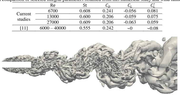
![Figure 8. Spanwise correlation of pressure coefficients. Wind tunnel results from [33] at Re = 63600](https://thumb-us.123doks.com/thumbv2/123dok_us/8676761.377713/8.595.44.558.317.563/figure-spanwise-correlation-pressure-coefficients-wind-tunnel-results.webp)