Labelling Strategies for Hierarchical Multi-Label
Classification Techniques
Isaac Trigueroa,b,∗, Celine Vensc
aDepartment of Respiratory Medicine, Ghent University, 9000 Ghent, Belgium bData Mining and Modelling for Biomedicine group, VIB Inflammation Research Center,
9052 Zwijnaarde, Belgium
cDepartment of Public Health and Primary Care, KU Leuven Kulak, 8500 Kortrijk,
Belgium
Abstract
Many hierarchical multi-label classification systems predict a real valued score for every (instance, class) couple, with a higher score reflecting more confidence thatthe instance belongs to that class. These classifiers leave the conversion of these scores to an actual label set to the user, who applies a cut-off value to the scores. The predictive performance of these classifiers is usually evaluated using threshold independent measures like precision-recall curves. However, several applications require actual label sets, and thus an automatic labelling strategy.
In this article, we present and evaluate different alternatives to perform the actual labelling in hierarchical multi-label classification. We investigate the selection of both single and multiple thresholds. Despite the existence of multiple threshold selection strategies in non-hierarchical multi-label clas-sification, they can not be applied directly to the hierarchical context. The proposed strategies are implemented within two main approaches: optimi-sation of a certain performance measure of interest (such as F-measure or hierarchical loss), and simulating training set properties (such as class dis-tribution or label cardinality) in the predictions. We assess the performance of the proposed labelling schemes on 10 datasets from different application domains. Our results show that selecting multiple thresholds may result in
∗Corresponding author. Tel : +32(0)9 331 36 93 Fax : +32(0)9 221 76 73
Email addresses: [email protected](Isaac Triguero),
an efficient and effective solution for hierarchical multi-label problems.
Keywords: Hierarchical multi-label classification, Threshold optimisation, Hierarchical loss, HMC-loss, F-measure
1. Introduction
Traditional classification problems deal with assigning a (single) class to an instance. However, many applications require assigning a set of classes (labels) to an instance. Examples are found in biology (e.g., gene function prediction [1, 2]), text or image classification [3, 4], etc. Multi-label classifi-cation algorithms have been proposed to tackle this task [5, 6, 7]. In many applications, the set of possible labels is structured as a hierarchy, represent-ing a superclass/subclass relation. For instance, gene functions are organised as a tree structure in MIPS’s FunCat hierarchy [8], or as a directed acyclic graph (DAG) in the Gene Ontology [9]. The corresponding classification task, that also takes into account this structure, is then called hierarchical multi-label classification (HMC) [10]. It thus involves predicting multiple and partial paths in a hierarchy of labels. Allowing partial paths means that the true and predicted paths need not necessarily to end in a leaf node. Sev-eral HMC algorithms have been proposed in the literature, e.g., [11, 12, 13]. They exploit the label set hierarchy when labelling instances. These systems also ensure (implicitly or using post-processing) that the hierarchy constraint is fulfilled in the predictions they make: whenever a class is predicted, its parent and ancestor classes are also predicted.
Rather than predicting an actual label set, most of the HMC algorithms actually predict a real valued prediction scorepifor every labelli, that reflects
the confidence that an instance should be annotated with label li. These
values can be easily converted into a label set by applying a threshold on them: if pi is above some threshold ti, then the instance is predicted to
belong to class li, otherwise not. To ensure that the predictions fulfil the
hierarchy constraint, it suffices to choose ti ≤tj whenever li is a super class
of lj.
larger pipeline of experiments, or the predicted image labels may be used as tags in image retrieval systems to locate images of interest. The objective of this article is to investigate and empirically compare different thresholding strategies.
HMC studies that fix the thresholds typically choose one threshold shared by all labels. In the non-hierarchical multi-label setting, however, studies ex-ist that choose a separate threshold per label [14, 15]. It is currently an open question how these two options compare in HMC, and this is addressed in this article. Non-hierarchical optimisation techniques can not be straight-forwardly applied in the HMC context, because of the aforementioned hier-archy constraint, and thus, we propose adapted techniques. Depending on the context, the user may want to set the thresholds such that the resulting classifier maximises predictive performance or such that training set proper-ties (such as class distribution) are reflected in the predictions. We consider both approaches. In order to apply the former approach, we first critically review several performance measures used in HMC to compare a predicted label set to a true label set: hierarchical loss, HMC-loss and micro-averaged F-measure.
The contributions of this work are as follows. First, we describe mea-sures that evaluate the predicted label sets, and we identify problems with the widely used (unweighted) hierarchical loss, which leads us to advise against its use (Section 2). Second, we devise a number of multiple-threshold-selection approaches for HMC (Section 3). Third, we empirically investigate the designed schemes and their single-threshold-selection counterparts on ten HMC datasets, showing that the multiple threshold approaches generally out-perform their single threshold variants, both in predictive out-performance and computationally (Section 4). We draw some conclusions and further research directions (Section 5).
2. Evaluating HMC classifiers
In HMC we obtain for every instance and every label a prediction. As mentioned in the introduction, this prediction is often real-valued. Given a hierarchy of k labels, we represent the predicted multi-label of an instance x
with a vector p = (p1, ..., pk) ∈ Rk. The label hierarchy can be represented
by a partial order ≤h that represents the superclass relationship. For all
following discussion, we assume that p fulfils the hierarchy constraint: pli ≥
plj whenever li ≤h lj.
In order to evaluate the predicted multi-labels in a test set, there are two possible strategies. The first strategy keeps the real-valued predictions, and evaluates them independently of any fixed thresholds. This is often done by constructing an average precision-recall curve (PR curve) and reporting the area under the curve. Precision gives the proportion of positive predictions that are positive, while recall gives the proportion of positive instances that are correctly predicted positive. A precision-recall curve plots the precision of a model as a function of its recall. While a threshold corresponds to a single point in PR space, by varying the threshold a curve is obtained. Vens et al. [11] and Pillai et al. [15] describe how to compute PR curves in the context of multiple labels.
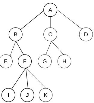
The second strategy is to convert the predicted multi-labels to binary vectors, by thresholding the predicted values, and to evaluate these binary multi-labels. In non-hierarchical multi-label classification several evaluation measures have been proposed for evaluating binary multi-labels. An overview is given by Tsoumakas et al. [6]. However, these measures are less suited for HMC tasks, exactly because they do not take into account the hierarchical structure in the labels. Kiritchenko et al. [16] formulate three requirements that should be fulfilled by a hierarchical evaluation measure (see the simple label hierarchy in Fig. 1, where {I,J} is indicated as the true multi-label to be predicted):
1. The measure should give credit to a partially correct classification. Thus, predicting node K should be better than predicting node C, as the prediction of K involves the path ABF that is part of the correct multi-label.
2. The measure should punish distant errors more heavily. This require-ment is split further into two parts:
(a) The measure should give a higher evaluation for correctly classi-fying one level down, than to stay at the parent. Thus, predicting
F should be better than predicting B.
(b) The measure should give a lower evaluation for incorrectly classi-fying one level down than to stay at the parent. Thus, predicting
H should be worse than predictingC.
3. The measure should punish errors at higher levels of the hierarchy more heavily. This means that, e.g. predicting D when the true label is C
Figure 1: Toy class hierarchy.
Examples of evaluation measures for binary multi-labels that do take into account a hierarchical label structure are hierarchical loss functions and a hierarchical extension of the F-measure. In the following, we represent the thresholded (binary) predicted multi-label of an instance with a vector
ˆ
p = (ˆp1, ...,pˆk) ∈ {0,1}k; similarly, we represent the true multi-label with a
vector l = (l1, ..., lk) ∈ {0,1}k. Without loss of generality, we also assume a
single root node in the hierarchy. In case of a collection of separate hierarchies (such as the Gene Ontology, which consists of three independent sub-graphs), this means that we create an artificial root node, to which all instances belong. This node then has as children the individual root nodes of the sub-hierarchies.
2.1. Hierarchical loss functions
The hierarchical loss (H-loss) function [17] was proposed specifically for HMC tasks. It assumes a tree structured label hierarchy. It is based on the Hamming or symmetric difference loss, which returns the symmetric differ-ence between the predicted and true multi-label vector for an instance. How-ever, the H-loss does not punish mistakes that have already been punished at a higher level in the hierarchy. In other words, whenever a classification mistake is made on a label in the hierarchy, the H-loss does not charge any loss for additional mistakes occurring in the subtree of that label:
H-loss(ˆp, l) = X
i=1..k
where anc(i) represents the set of ancestors of node i, and c1, ..., ck > 0 are
fixed cost coefficients. Cesa-Bianchi et al. [18] propose two variants of the H-loss function: uniform H-H-loss with all coefficients set to one, and normalised H-loss, where each node’s cost is equally split recursively among its children. The latter is achieved by setting the coefficients as follows: croot = 1, and for
the other nodes i in the hierarchy ci = cj/|child(j)| with j the parent of i.
For the label hierarchy in Fig. 1, this yields cA = 1, cB = cC = cD = 1/3, cE =cF =cG =cH = 1/6, andcI =cJ =cK = 1/18.
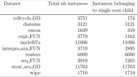
In practice, most HMC papers that use the H-loss use the uniform variant (e.g., [19, 20, 21, 22, 23, 13, 24]). Here, we identify two problems with this H-loss variant. First, surprisingly, none of the requirements by Kiritchenko et al. [16] is met by the uniform H-loss. This can be easily verified by calculating the H-loss for the examples given above. Second, it turns out that making zero predictions (i.e., predicting only the root, which is by default present in all instances) often results in a very good uniform H-loss score. Let us call a class that appears in the first level (i.e., directly under the root) of the class hierarchy a level1 class. If an instance has target labels that all belong to paths that pass through a single level1 class, then an empty prediction yields a H-loss of 1. This is the second best value that can be obtained. Only a completely perfectly predicted multi-label can yield a H-loss of 0. Since level1 classes are the most general classes in the taxonomy, it is to be expected that, even though an instance belongs to many paths, these paths will often pass through a single level1 class, and the multiple labels will only differentiate at lower, more specialised, levels of the hierarchy1. For instance, in gene function annotation, a gene involved in “aerobic respiration” (FunCat category 02.13.03) and in “photosynthesis” (02.30), which both belong to the level1 class “energy” (02) may be less likely to also have functions related to other level1 classes like “storage protein” (04) or “transcription” (11). Table 1 confirms the high rate of instances whose class(es) only pass(es) through a single level1 class. Clearly, the uniform H-loss function does not achieve what one would expect intuitively from a loss function designed for hierarchical classification. Cerri et al. [13] have observed that uniform H-loss can lead to results contradicting those of other evaluation measures, when comparing global versus local HMC prediction models.
1Remark that for hierarchical single-label classification tasks, there is always only a
Table 1: Number of instances belonging to a single root child.
Dataset Total nb instances Instances belonging to single root child cellcycle GO 3751 174
diatoms 3121 3121
enron 1649 319
expr FUN 3779 1162 imclef07a 11006 11006 interpro ara FUN 3719 2895 reuters 6000 6000 seq FUN 3919 1265 struc ara GO 11763 11763
wipo 1710 1710
The normalised H-loss mostly solves the issues discussed above, because (1) the coefficients decrease with increasing depth in the hierarchy, and (2) the total loss obtained for mistakes in a subtree can never exceed the cost associated with the root of the subtree. However, it still has a tendency to favour empty predictions, when used in a threshold selection scheme (see Section 4). Cesa-Bianchi et al. [18] list another disadvantage of this function: if the hierarchy has large branching factors in the upper levels, then the co-efficients quickly become very small, which in turn yields very small H-loss values and makes it difficult to conduct comparisons among algorithms. Nev-ertheless, it should be stressed that the normalised H-loss should be preferred over the uniform H-loss.
Bi and Kwok [25] criticise H-loss, because it can never meet requirement 2b of Kiritchenko et al. [16]: when comparing two false positive predictions, where one prediction is more specific than the other, intuitively, the more specific prediction should receive a lower evaluation than the (more prudent) general one. However, this is in contrast to the idea behind H-loss, which gives them an equal evaluation. In response to this, Bi and Kwok designed the HMC-loss, which is also applicable to DAG label hierarchies:
HMC-loss(ˆp, l) =α X i=1..k: ˆpi=0,li=1
ci+β
X
i=1..k: ˆpi=1,li=0
ci, (2)
wherec1, ..., ck>0 are fixed cost coefficients, which are defined as in the
nor-malised H-loss for tree hierarchies. For DAGs, the cost for non-root nodes is set as follows: ci =
P
coef-ficients α and β allow a cost-sensitive learning setting, where false positives and false negatives are weighted differently. When α=β = 1, the HMC-loss becomes equal to a weighted Hamming-loss, or to the uniform H-loss that does not disregard subtrees whenever a mistake is counted. The HMC-loss effectively solves the empty prediction issue of H-loss, because instead of only punishing the root node, every node belonging to the multi-label con-tributes to the loss. Moreover, all requirements for a hierarchical evaluation measure [16] are fulfilled.
2.2. Hierarchical F-measure
Precision and recall are traditionally defined for single-label classification problems. As these measures provide complementary information, they are often combined, resulting in the F-measure:
Fβ =
(β2+ 1)×precision×recall
β2×precision+recall , β ≥0 (3)
Parameterβ weighs the importance of precision versus recall. In the rest of the paper, we use β = 1, resulting in the harmonic mean of precision and recall.
When dealing with multiple classes, precision, recall and F-measure are averaged. There are two strategies to calculate the average. Consider a prediction matrix, P, where each row represents an instance, each column a label, and the values the corresponding binary predictions. The macro-average computes the above measures for each column individually and then averages them over the columns. Thus, each class obtains an equal weight in the calculation. In contrast, the micro-average looks at all cells of the predic-tion matrix together. Micro-averaged precision (denoted by precisionm) is then the proportion of positively predicted cells that are positive and micro-averaged recall (recallm) is the proportion of positive cells that are correctly
predicted positive. The corresponding micro-averaged F1 measure (F1m) is
given by:
F1m = 2×precision
m×recallm
precisionm+recallm (4)
While the macro-average gives an equal weight to each class, and thus tends to over-estimate the importance of rare classes, the micro-average im-plicitly gives more weight to more frequent classes. In the hierarchical setting, it thus makes more sense to consider the Fm
al. [11] showed that PR curves generated from micro-averaged precision and recall can better capture overfitting issues. If the true label set fulfils the hier-archy constraint (which we assume in this article), i.e., whenever an instance belongs to some class it also belongs to the parent class, then Kiritchenko et al. [16] call the corresponding micro-averaged precision, recall and F1 the hierarchical precision, recall andF1 measures, respectively. In addition, they
show that the hierarchical F1 measure fulfils the requirements for
hierarchi-cal evaluation measures. Other papers that use the hierarchihierarchi-cal F1 measure
include the work of Valentini [26] and Cesa-Bianchi et al. [27]. This measure can be applied to both tree and DAG structured hierarchies.
3. Threshold selection methods for HMC problems
In this section we present different alternatives to perform the final la-belling of an HMC problem given a set of real-valued scores for the potential classes.
Let us assume we have trained a HMC classifier with a given training datasetT RS. Then, we classify a validation setV S, i.e. a set ofNv instances
that did not play any role in the construction of the classifier, and for which the true multi-labels are known, i.e., we dispose of a binary matrixLval that
indicates for each validation instance the actual labels. Moreover, we classify a test set T S composed ofNt instances where the labels are unknown. As a
result, we obtain two prediction matricesPval ={{p11, .., p1k}, ...,{p Nv
1 , .., p Nv
k }}
and Ptest = {{p11, .., p1k}, ...,{p Nt
1 , .., p Nt
k }} that are composed of Nv and Nt
prediction vectors pi, respectively.
The final objective is to determine the best labelling of theT S instances. To do this, we utilise the Pval matrix as reference and we look for the best
thresholds that convert it into a binary prediction matrix ˆPval, which is
eval-uated against the actual labelsLval. Then, the learned thresholds are applied
to the Ptest matrix. There are two aspects in determining the best
thresh-olding strategy.
single and multiple thresholds selection. Both approaches are optimisation schemes that are generically illustrated in Algorithms 1 and 2.
Algorithm 1 Generic STS pseudo-code
Require: A validation prediction matrixPval.
Ensure: A global threshold t.
1: CutPoints= all different values from Pval sorted in ascending order. 2: bestThreshold = -1
3: bestPerformance = worst value //e.g.,∞if performance is to be minimised
4: for each cutpoint in CutPoints do
5: performance = ComputePerformance(Pval, cutpoint,Lval) 6: if betterThan(performance,bestPerformance) then 7: bestPerformance = performance
8: bestThreshold = cutpoint;
9: end if
10: end for
11: return bestThreshold
• Single-threshold selection (STS) consists of computing a single cut-off per dataset that optimises some value. A threshold t that is shared between all the classes is obtained and used to transform Pval into
ˆ
Pval. Most HMC classifiers provide aPval that preserves the hierarchy
constraint, so that the probability of belonging to label lj cannot be
higher than the probability associated to li whenever li ≤h lj (li is an
ancestor of lj). Therefore, the application of a single threshold over all
classes keeps the hierarchy constraint.
• Multiple-thresholds selection (MTS) optimises a threshold ti for every
label of a dataset, resulting in a vector t = (t1, ..., tk). As such, the
STS approach can be considered a particular case of the MTS in which all the thresholds are forced to be equal. However, in this case, the hierarchy constraint must be ensured during the selection process by keeping any threshold ti ≤tj whenever li ≤h lj.
Algorithm 2 Generic MTS pseudo-code
Require: A validation prediction matrixPval. Ensure: A threshold vector t= (t1, ..., tk).
1: for each class i do
2: CutPoints[i] = all different values from column i of Pval sorted in
as-cending order.
3: end for
4: bestThresholdVector = [-1,-1,...,-1]
5: bestPerformance = worst value //e.g.,∞if performance is to be minimised
6: for each possible threshold vector t from CutPoints do
7: performance = ComputePerformance(Pval,t,Lval) 8: if betterThan(performance,bestPerformance) then 9: bestPerformance = performance
10: bestThresholdVector = t;
11: end if
12: end for
13: return bestThresholdVector
so, O(Nv×k). In general, however, the number of possible threshold values
is lower than Nv ×k because of repeated values. The complexity of STS
can easily be reduced though, at the cost of a decrease in accuracy, by using a sub-optimal approach. This approximation may consist of the evaluation of limited number of possible candidate threshold values, which are equally distributed in the range of the score values. For instance, if the score values belong to the range [0,1], we may investigate 100 thresholds as {0.01, 0.02, ..., 1}.
In MTS, for every classliwe have to find a thresholdti ∈[min(Pval(i)), max(Pval(i))], where Pval(i) represents the column vector i of Pval. Thus, the number of
processed. Thus, both for decomposable and non-decomposable measures, the hierarchy has a positive influence on computational complexity.
Obtaining single or multiple thresholds according to the validation set does not guarantee that the threshold/s is/are the most suitable for the test set, due to overfitting phenomena. For this reason, in the proposed MTS approaches, we do not pursue optimal approaches that may not be feasible in time, but rather efficient search processes that guarantee that only coherent threshold vectors (w.r.t. the hierarchy constraint) are evaluated.
The second aspect in the thresholding strategy is how to compute the performance, which corresponds to the procedure ComputePerformance in Algorithms 1 and 2:
• Compute the predictive performance in the validation set, using the evaluation measure that will be used to evaluate the test set predictions (Section 3.1).
• Reflect training or validation set properties in the test set predictions.
We now discuss each of these in detail.
3.1. Optimising the evaluation measure
One obvious strategy is to optimise the performance measure that will be used in the end to evaluate the test set predictions. In the experiments (Section 4), three evaluation measures will be used that were discussed in Section 2: the normalised H-loss, the HMC-loss and the F1m. Optimising them under the STS scheme is straightforward following Algorithm 1. For every possible threshold value, calculate the corresponding measure, and take the threshold that yielded the best value. However, under the MTS scheme, the optimisation process becomes more complicated. In what follows, we propose three optimisation processes associated to the hierarchical loss (Sec-tion 3.1.1), the HMC-loss (Sec(Sec-tion 3.1.2) and the micro-averaged F-measure (Section 3.1.3), respectively.
3.1.1. Multiple Threshold Selection for the Normalised Hierarchical Loss.
We start by fixing the root’s threshold to zero: every instance belongs to the root, so any threshold between 0 and 1 would be valid. However, as the thresholds need to increase while going down the hierarchy, it is better to set the root threshold as low as possible. Then we recursively move to the child nodes, and for each of these nodes select the threshold that minimises the normalised H-loss, only considering the nodes on the path from this node to the root, and only considering candidate thresholds equal to or higher than the parent’s threshold, to enforce the hierarchy constraint. This efficient pro-cedure results in an optimal threshold vector, because the total loss incurred in the subtree of a node can never exceed the loss associated with the node itself.
The procedure is outlined in Algorithm 3. The N ormHLoss function calculates the normalised H-loss given a label matrix, a prediction matrix on which it applies the previously calculated and current thresholds, and the hierarchy path from the current node to the root.
For DAGs datasets we set the coefficients as in the HMC-loss (See Section 2.1). However, the optimality is not guaranteed in this case, because the coefficients may increase while moving down in the hierarchy.
3.1.2. Multiple Threshold Selection for the HMC-loss
The HMC-loss simply adds the losses (false positives and false negatives) for each label of the hierarchy. As stated by Equation 2, it takes into account the hierarchy by using coefficients that decrease with the depth. As such, this measure could be decomposed over the different classes. However, an independent optimisation per class, as proposed for the normalised H-loss, is not applicable, even though a top-down approach is considered. The reason is that now the total loss incurred in the subtree of a nodecan exceed the loss associated with the node itself. For example, in Fig. 1, node B has coefficient 1/3, but the subtree below it has total coefficient of 1/2. Thus, the subtree needs to be considered when selecting a threshold for node B.
Algorithm 3 MTS for the Normalised H-loss
Require: A validation prediction matrixPval and label matrix Lval. Ensure: A threshold vector t= (t1, ..., tk).
1: bestThresholds[1,...,k] = [0,-1,...,-1]
2: for each non-root node i (top-down approach) do 3: bestLoss =∞
4: Hi = hierarchy path starting in the root node and ending in i
5: CutPoints = all different values from the column of Pval that
corre-spond to i, that are equal to or larger than the threshold selected for
i’s parent
6: for eachcutpoint in CutPoints do
7: loss = N ormHLoss(Pval, Lval, cutpoint, bestT hresholds, Hi) 8: if loss< bestLoss then
9: bestLoss = loss
10: bestThresholds[i] = cutpoint
11: end if
12: end for
13: end for
constraint: the threshold forishould be equal to or larger than the threshold for i’s parent.
Algorithm 4 MTS for the HMC-loss
Require: A validation prediction matrixPval and label matrix Lval. Ensure: A threshold vector t= (t1, ..., tk).
1: bestThresholds[1,...,k] = [0,-1,...,-1]
2: for each non-root node i (top-down approach) do 3: bestLoss =∞
4: Subi = subtree of nodei (including i itself)
5: CutPoints = all different values from the columns of Pval that
corre-spond to Subi, that are equal to or larger than the threshold selected
for i’s parent
6: for eachcutpoint in CutPoints do
7: loss = HM CLoss(Pval, Lval, cutpoint, Subi) 8: if loss< bestLoss then
9: bestLoss = loss
10: bestThresholds[i] = cutpoint
11: end if
12: end for
13: end for
14: return bestThresholds
Note that this approach is sub-optimal: if the optimal threshold would be 0.6 for node B, and 0.7 for nodes E, F, I, J and K, then this can only be found if, during the selection of B’s threshold, using 0.6 for all nodes (too many false positives) is better than 0.7 for all nodes (too many false negatives).
3.1.3. Multiple Threshold Selection for the micro-averaged F-measure
fixed. The main problem in extending this approach towards HMC, is that increasing the value of a single threshold will violate the hierarchy constraint. Indeed, if a threshold for node iis increased, all thresholds corresponding to
i’s descendants need to be increased as well, as they should be larger than or equal to i’s threshold. Here, we propose to set the thresholds of the descen-dants equal to the threshold being updated, thus keeping the computational cost advantage, at the cost of providing a sub-optimal solution, in the same sense as when optimising the HMC-loss.
Following Pillai’s notation for sake of clarity, let t = (t1, ..., tk) denote a
specific value of the thresholds, andT = (T1, ..., Tk) the thresholds considered
as variable. Let us assume that all the score prediction vectors per class
Pval(i) = {Pval(i,0), Pval(i,1), ..., Pval(i, Nv)} have been sorted in ascending
order, so that, Pval(i, j) ≤ Pval(i, j + 1),∀j = 1, ..., Nv −1. Algorithm 5
presents the pseudo-code of the modified algorithm. In what follows we describe the main changes performed to the method, referring to the lines in the pseudo-code.
First of all, all the thresholds ti are originally initialised to any random
value between (0, Pval(i,0)). In contrast, we set all thresholds to zero, in
order to ensure the hierarchy constraint is fulfilled at the start.
Then, based on two main properties, Pillai et al. demonstrated that an iterative updating process is globally optimal. In this process, each threshold
Ti is increased to any value that locally increases the Fβm, while keeping all
the otherTj, j 6=ifixed, until no improvement is achieved by changing any of
the thresholds (lines 6-29). This means that even though the Fβm cannot be decomposed over classes, the optimisation can be implemented in an iterative way, and thereby reducing complexity.
In the original proposal, everyTi is checked with all the values contained
in the prediction vectorPval(i). Lines 2-4 extract all potential cut points for
every class from Pval.
When investigating the value of a given Ti, we have to check that the
fixed threshold values of the descendants of label li satisfy the hierarchy. In
this way, the descendant thresholds may become variable Td, whereldis any
children of class li (See lines 12-16).
When the best threshold has been determined for the current Ti and
its associated Td’s, the algorithm checks if this optimisation has yielded a
better performance. If yes, the thresholds values of ti and its descendants
Algorithm 5 MTS for the micro-averaged F-measure Require: A validation prediction matrixPvaland label matrixLval.
Ensure: A threshold vectort= (t1, ..., tk).
1: bestThresholds[1,...,k] = [0,0,...,0] 2: forall classesdo
3: CutPoints[i] = All different values from columniofPvalsorted in ascending order.
4: end for
5: bestPerformance =−∞
6: repeat
7: updated <−f alse
8: foreach nodei(top-down approach)do
9: Descendants=listOfDescendants(i) 10: forall valuesTiinCutP oints[i]≥tido
11: %Enforce hierarchy
12: foreach nodedinDescendantsdo
13: ifTi> tdthen
14: Td=Ti
15: end if
16: end for
17: performance=Fm
β (Pval, Lval,{t1, .., Ti, Td, ..., tk}) withTd=Tifor all descendants
18: if better than(perf ormance, bestP erf ormance)then
19: bestPerformance = performance
20: bestThresholds=Ti,Td(ifTdhas been modified);
21: end if
22: end for
23: ifbetter than(perf ormance, bestP erf ormance)then
24: {ti, td}=bestT hresholds
25: updated=true
26: end if
27: end for
parent of the current analysed label is already fixed.
3.2. Reflecting training set properties
Apart from optimising a certain error measure of interest, a second po-tential strategy is to choose thresholds in such a way that some properties of the training or validation sets remain in the predictions of the test set. Specifically, we analyse two different strategies:
• To reflect the positive/negative distributions for each label in the re-sulting predictions (Subsection 3.2.1).
• To make the label cardinalities as similar as possible (Subsection 3.2.2).
The aim of these proposals is to check whether a simple and fast approach may yield successful thresholds, even though performance measures are not considered.
3.2.1. Reflecting class distribution
The idea behind this strategy is to perform a STS or MTS process in which the function to be optimised is the distance to the true class distribution. The thresholds are chosen based on the validation set, in such a way that they result in a positive/negative split for each class that is as close as possible to the true positive/negative split. Therefore, the true class distribution is also estimated from the validation set (and not from the training set, since this might introduce noise if the training set class distributions differ slightly from those of the validation set). To do so, we use the label matrix Lval and
for each class i compute the percentage of positive instancesCDi.
Under STS, we follow Algorithm 1 in which the computePerformance
function computes, for a given cut point and the prediction matrix Pval, the
predicted percentage of positive instances CDi0 for each label. The threshold that minimises the Euclidean distance between the CD and CD0 vectors is chosen.
A very similar labelling strategy has been used in text categorisation, it is referred to as PCut by Yang [32], and as proportional assignment by Lewis and Ringuette [33] and Wiener et al. [34]. The difference is that these authors did not use a separate validation set to determine the thresholds, they imme-diately pick the positive/negative split in the test set that corresponds to the class distribution of the training set. The disadvantage of their approach is that, if the test set is changed (e.g., it grows because new instances become available), then the prediction of individual test instances may change.
3.2.2. Reflecting label cardinalities
This alternative aims at reflecting the label cardinality of the validation samples. Label cardinality is defined as the average number of labels associ-ated with an instance [6]. This is relassoci-ated to the strategy used in [35] where the authors compared the label cardinality of the predictions in the test set to the label cardinality over the training set. Instead of using an averaged label cardinality, we compare instance per instance the true number of labels and the predicted number of labels over a validation set.
In STS, we count for each validation instance how many labels are present, obtaining a vector of true label counts per example LCi, where 1 < i < n.
When analysing the different thresholds, we compute the resulting predicted label counts LCi0. Afterwards, the Euclidean distance between both vectors is minimised.
An MTS label cardinality approach is not applicable, since label cardi-nalities are computed per instance, and not per class.
4. Experimental Study
In this section, we start by defining the experimental set-up in Section 4.1: we detail the problems chosen for the experimentation, the measures employed to evaluate the performance of the algorithms and finally, the sta-tistical tests conducted to contrast the results obtained. Then, Section 4.2 shows the results analysing the different proposed alternatives to perform the final labelling in HMC problems.
4.1. Experimental set-up
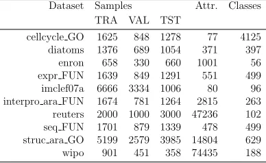
Table 2: Properties of the datasets considered.
Dataset Samples Attr. Classes TRA VAL TST
cellcycle GO 1625 848 1278 77 4125 diatoms 1376 689 1054 371 397
enron 658 330 660 1001 56
expr FUN 1639 849 1291 551 499 imclef07a 6666 3334 1006 80 96 interpro ara FUN 1674 781 1264 2815 263 reuters 2000 1000 3000 47236 102 seq FUN 1701 879 1339 478 499 struc ara GO 5199 2579 3985 14804 629 wipo 901 451 358 74435 188
gene function prediction. These datasets have been collected from freely-available repositories234. Two of the gene function prediction datasets have annotations coming from the gene ontology (GO) [9]. This ontology forms a directed acyclic graph instead of a tree: each node can have multiple parents. We denote them as GO datasets.
All these data sets are originally split into a training and a test set. For those datasets for which no validation set is available, we set aside a random subset of 1/3 of the training set as validation set. Table 2 details the main properties of these datasets. It shows the number of instances in the different partitions, number of attributes (Attr.) and number of classes.
In our experiments, we use the Clus-HMC-Ens algorithm [2] as a repre-sentative state-of-the-art HMC classifier. It constructs a random forest of 50 predictive clustering trees. Each individual tree makes a prediction for the complete multi-label. All the predictions provided by this method preserve the hierarchy constraint. In order to optimise the labelling strategies, a ran-dom forest is first built on the training set and tested on the validation set. Afterwards, the final model is built on the combination of training and vali-dation sets, and tested on the test set. As a result, we obtain two prediction matrices Pval and Ptest.
The STS and MTS approaches will be investigated under each of the 3
2
https://dtai.cs.kuleuven.be/clus/hmcdatasets/ 3
https://dtai.cs.kuleuven.be/clus/hmc-ens/ 4
different schemes presented before: optimising an error measure (EM), class distribution (CD) and label cardinalities (LC). We will denote these ap-proaches as EM(), CD() and LC(), indicating STS or MTS versions between brackets. We will use three error measures: normalised H-loss, HMC-loss and the micro-averaged F-measure with β = 1 (Fm
1 ). For the HMC-loss, as in
[25], we setα=λ·βwhile keepingα+β = 2, whereλbecomes the parameter that balances the misclassification cost between positive and negative exam-ples and it is set to the ratio of negative examexam-ples in relation to the positive ones: λ = #negatives/#positives. We also test two different settings for the STS approach, either using all available threshold values (optimal so-lution) or using a binning procedure. For the approximate STS approach, we use 100 values equally distributed in [0,1], which is the output range of Clus-HMC-Ens. Moreover, we compute the run time spent by the different analysed approaches in order to compare their complexity in practice. Ten executions of each algorithm have been performed and their run time has been averaged. All the experiments have been carried out on an Intel(R) Xeon(R) CPU E5-1650 v2 at 3.50GHz without any kind of parallellization.
To provide statistical support for the analysis of results performed, we will apply hypothesis testing techniques. More specifically, we make use of non-parametric tests that were suggested in the studies presented in [36, 37] for machine learning applications. The Wilcoxon test [38] will be used to perform pairwise comparisons between the STS and MTS labelling schemes. It will be adopted considering a level of significance of α= 0.05.
information about these tests and other statistical procedures can be found at http://sci2s.ugr.es/sicidm/.
4.2. Results and analysis
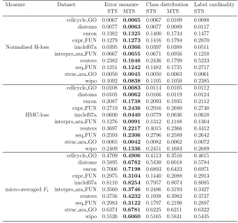
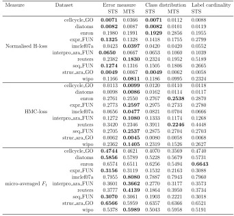
Tables 3 and 4 collect the obtained results in the validation and test set, respectively. In both tables, the best result for each dataset and perfor-mance measure has been highlighted in bold-face. We present the validation set results to analyse the generalisation capabilities of the methods. Never-theless, the conclusions related to the performance of the methods need to be evaluated in the test set.
This study is divided into two parts. We first compare STS and MTS approaches across the proposed optimisation strategies (Section 4.2.1). Af-terwards, we perform a global study to determine which is the best alternative according to every performance measure considered (Section 4.2.2). In both studies, we evaluate the resulting threshold selection techniques in terms of predictive performance, influence of the overfitting phenomena and required run time.
Note that for the label cardinality and class distribution approaches we computed the threshold/s once, and then the computed thresholds are used to compute the final performance with the three considered measures. However, for the error measure optimisation process we have independent threshold/s for each measure.
4.2.1. STS vs. MTS
This subsection compares the STS and MTS approaches. As commented before, there is no MTS variant for the label cardinality strategy. Thus, only the error measure and class distribution approaches are included in the following analysis.
To significantly characterise the differences between STS and MTS ap-proaches, the Wilcoxon signed-ranks test has been applied for the possible settings. A total of 12 Wilcoxon tests are conducted to compare STS and MTS approach depending on the performance measure, the optimisation strategy and the considered dataset (validation or test). Table 5 presents the associated p-values for each statistical test conducted. Significant differ-ences (α = 0.05) are stressed in bold-face. According to this table we can state that:
Table 3: Results obtained at the validation set
.
Measure Dataset Error measure Class distribution Label cardinality STS MTS STS MTS STS
cellcycle GO 0.0067 0.0065 0.0067 0.0109 0.0088 diatoms 0.0077 0.0063 0.0077 0.0089 0.0117 enron 0.1382 0.1325 0.1400 0.1734 0.1477 expr FUN 0.1279 0.1273 0.1416 0.1794 0.2870 Normalised H-loss imclef07a 0.0395 0.0366 0.0397 0.0388 0.0511 interpro ara FUN 0.0667 0.0655 0.0671 0.0956 0.1210 reuters 0.2382 0.1646 0.2436 0.1799 0.5233 seq FUN 0.1251 0.1242 0.1482 0.1735 0.2717 struc ara GO 0.0050 0.0045 0.0050 0.0063 0.0061 wipo 0.1092 0.0838 0.1105 0.1050 0.2385 cellcycle GO 0.0108 0.0083 0.0114 0.0105 0.0112 diatoms 0.0105 0.0062 0.0166 0.0119 0.0124 enron 0.2087 0.1738 0.2093 0.1935 0.2112 expr FUN 0.2719 0.2436 0.2916 0.2680 0.2740 HMC-loss imclef07a 0.0600 0.0440 0.0779 0.0636 0.0610 interpro ara FUN 0.1276 0.0991 0.1312 0.1188 0.1304 reuters 0.3697 0.2217 0.4015 0.2366 0.4412 seq FUN 0.2593 0.2306 0.2796 0.2589 0.2642 struc ara GO 0.0065 0.0042 0.0082 0.0062 0.0072 wipo 0.2409 0.1336 0.2451 0.1683 0.2689 cellcycle GO 0.4709 0.4906 0.4113 0.3516 0.4615 diatoms 0.5895 0.6782 0.5430 0.6018 0.5784 enron 0.7006 0.7198 0.6893 0.6423 0.6971 expr FUN 0.2975 0.3104 0.1440 0.2088 0.2913 imclef07a 0.8110 0.8254 0.7957 0.8074 0.8085 micro-averagedF1 interpro ara FUN 0.3560 0.3746 0.2486 0.3193 0.3427
Table 4: Results at the test set
.
Measure Dataset Error measure Class distribution Label cardinality
STS MTS STS MTS STS
cellcycle GO 0.0071 0.0366 0.0071 0.0112 0.0088 diatoms 0.0082 0.0087 0.0082 0.0101 0.0119 enron 0.1980 0.1991 0.1929 0.2856 0.1955 expr FUN 0.1325 0.1328 0.1418 0.1755 0.2799 Normalised H-loss imclef07a 0.0423 0.0397 0.0420 0.0420 0.0552 interpro ara FUN 0.0650 0.0667 0.0653 0.1060 0.1039 reuters 0.2382 0.1830 0.2324 0.1952 0.5189 seq FUN 0.1274 0.1316 0.1505 0.1806 0.2665 struc ara GO 0.0049 0.0067 0.0049 0.0062 0.0058 wipo 0.1166 0.0811 0.1186 0.0995 0.2324 cellcycle GO 0.0113 0.0099 0.0120 0.0110 0.0118 diatoms 0.0098 0.0086 0.0162 0.0114 0.0117 enron 0.2761 0.2550 0.2767 0.2538 0.2870 expr FUN 0.2773 0.2597 0.2975 0.2733 0.2780 HMC-loss imclef07a 0.0656 0.0477 0.0821 0.0704 0.0666 interpro ara FUN 0.1272 0.1080 0.1333 0.1174 0.1268 reuters 0.3420 0.2346 0.3911 0.2246 0.4448 seq FUN 0.2705 0.2537 0.2875 0.2704 0.2703 struc ara GO 0.0062 0.0045 0.0080 0.0058 0.0068 wipo 0.2362 0.1405 0.2319 0.1526 0.2627 cellcycle GO 0.4744 0.4621 0.4070 0.3569 0.4740 diatoms 0.5856 0.5789 0.5228 0.5679 0.5731 enron 0.6574 0.6511 0.6256 0.5494 0.6643
expr FUN 0.3156 0.3119 0.1532 0.2163 0.3088 imclef07a 0.7955 0.8080 0.7887 0.7943 0.7960 micro-averagedF1 interpro ara FUN 0.3601 0.3662 0.2770 0.3177 0.3573
reuters 0.3777 0.4139 0.1864 0.3950 0.3734 seq FUN 0.3070 0.3061 0.1903 0.2221 0.3018 struc ara GO 0.6566 0.5959 0.6357 0.6366 0.6521 wipo 0.5378 0.5989 0.5043 0.5958 0.5191
Table 5: Wilcoxon tests: MTS vs. STS for each strategy. The obtained p-values are presented.
Error measure Class distribution MTS vs STS Validation Test Validation Test Normalised H-loss 0.0020 >= 0.2 >= 0.2 >= 0.2 HMC-loss 0.0020 0.0020 0.0020 0.0020
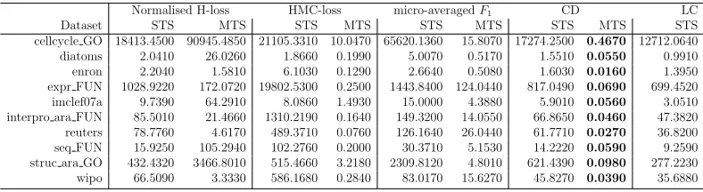
Table 6: Run time spent by the different optimisation techniques (in seconds).
Normalised H-loss HMC-loss micro-averagedF1 CD LC
Dataset STS MTS STS MTS STS MTS STS MTS STS
cellcycle GO 18413.4500 90945.4850 21105.3310 10.0470 65620.1360 15.8070 17274.2500 0.4670 12712.0640
diatoms 2.0410 26.0260 1.8660 0.1990 5.0070 0.5170 1.5510 0.0550 0.9910
enron 2.2040 1.5810 6.1030 0.1290 2.6640 0.5080 1.6030 0.0160 1.3950
expr FUN 1028.9220 172.0720 19802.5300 0.2500 1443.8400 124.0440 817.0490 0.0690 699.4520
imclef07a 9.7390 64.2910 8.0860 1.4930 15.0000 4.3880 5.9010 0.0560 3.0510
interpro ara FUN 85.5010 21.4660 1310.2190 0.1640 149.3200 14.0550 66.8650 0.0460 47.3820
reuters 78.7760 4.6170 489.3710 0.0760 126.1640 26.0440 61.7710 0.0270 36.8200
seq FUN 15.9250 105.2940 102.2760 0.2000 30.3710 5.1530 14.2220 0.0590 9.2590
struc ara GO 432.4320 3466.8010 515.4660 3.2180 2309.8120 4.8010 621.4390 0.0980 277.2230
wipo 66.5090 3.3330 586.1680 0.2840 83.0170 15.6270 45.8270 0.0390 35.6880
the test set. This fact shows that the generalisation capabilities of the MTS with F-measure and normalised H-loss are rather limited. Never-theless, for the HMC-loss we can state that the MTS approach is the most suitable approach.
• When the CD optimisation is considered, no significant differences are found between the methods in both validation and test phase, except for the HMC-loss, in which the MTS class distribution optimisation has provided statistically better results.
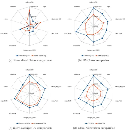
To compare both STS and MTS in terms of efficiency, Figure 2 depicts star plots representing the average run time obtained in each dataset for the four STS vs. MTS comparisons considered (note that ClassDistribution is only run once). This star plot presents the run time as the distance from the center; thus, a lower area determines the most efficient methods. For sake of clarity, logarithm scale has been used to counter the skewness between the run times in the different datasets. Table 6 collects the complete list of run time values in seconds. The fastest technique for each dataset is highlighted in bold-face.
In 3 out of the 4 plots, we can observe that STS requires more time to compute a single threshold than MTS to compute often hundreds of thresh-olds. To fully understand these results, several points must be clarified:
(a) Normalised H-loss comparison (b) HMC-loss comparison
[image:26.612.117.547.173.625.2](c) micro-averagedF1comparison (d) ClassDistribution comparison
approaches, they must analyse all the possible thresholdsNv×k,
inde-pendently of the relation between classes.
• MTS approaches have the advantage that they can prune many of the cut points, due to the followed top-down approach and the hierarchy constraint checks.
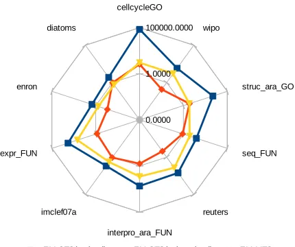
• Nevertheless, as stated before, the complexity of the STS approach could be further reduced by using a sub-optimal approach. Figure 3 presents a comparison of the run time required between a non-optimal STS approach, the optimal STS and the proposed MTS model. This figure considers the EM optimisation of the micro-averagedF1 measure
as an example. We can see that such kind of sub-optimal approach (fixing 100 thresholds) provides a reduced run time. However, the micro-averagedF1 obtained by the sub-optimal STS is always less than
[image:27.612.198.413.376.556.2]the optimal approach, and a statistical comparison with Wilcoxon test results in a p-value=0.0039.
Figure 3: micro-averaged F1 run time comparison for STS sub-optimal approach. Log scale is utilised.
4.2.2. Global analysis
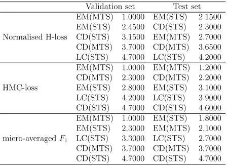
Table 7: Average Friedman Rankings sorted from the best to the worst
Validation set Test set EM(MTS) 1.0000 EM(STS) 2.1500 EM(STS) 2.4500 CD(STS) 2.3000 Normalised H-loss CD(STS) 3.1500 EM(MTS) 2.7000 CD(MTS) 3.7000 CD(MTS) 3.6500 LC(STS) 4.7000 LC(STS) 4.2000 EM(MTS) 1.0000 EM(MTS) 1.2000 CD(MTS) 2.3000 CD(MTS) 2.2000 HMC-loss EM(STS) 2.8000 EM(STS) 3.1000 LC(STS) 4.2000 LC(STS) 3.9000 CD(STS) 4.7000 CD(STS) 4.6000 EM(MTS) 1.0000 EM(STS) 1.8000 EM(STS) 2.3000 EM(MTS) 2.1000 micro-averagedF1 LC(STS) 3.3000 LC(STS) 2.7000
CD(MTS) 3.7000 CD(MTS) 3.7000 CD(STS) 4.7000 CD(STS) 4.7000
performance measure. In this table, algorithms are ordered from the best (lowest) to the worst (highest) ranking.
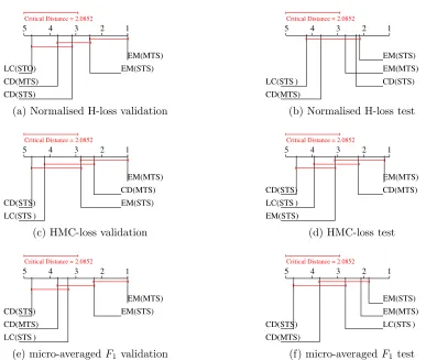
The Friedman test has detected statistically significant differences be-tween the performance of all the labelling schemes. Thus, the Nemenyi post hoc test is applied to characterise the significant differences. Figure 4 plots the corresponding average ranks diagrams.
Finally, Figure 5 establishes a global comparison in terms of run time with all the considered methods.
From these figures and Table 7, we can conclude that:
• For normalised H-loss, EM techniques together with CD(STS) rank in the first positions. The difference between EM techniques and the rest of alternatives is more accentuated in the validation phase than in the test phase. It may indicate that, for the considered datasets, EM techniques have suffered from overfitting.
5 4 3 2 1 EM(MTS) EM(STS) CD(STS) CD(MTS) LC(STO)
Critical Distance = 2.0852
(a) Normalised H-loss validation
5 4 3 2 1
EM(STS) EM(MTS) CD(STS) CD(MTS)
LC(STS )
Critical Distance = 2.0852
(b) Normalised H-loss test
5 4 3 2 1
EM(MTS) CD(MTS) EM(STS) LC(STS )
CD(STS)
Critical Distance = 2.0852
(c) HMC-loss validation
5 4 3 2 1
EM(MTS) CD(MTS)
EM(STS) LC(STS ) CD(STS)
Critical Distance = 2.0852
(d) HMC-loss test
5 4 3 2 1
EM(MTS) EM(STS)
LC(STS ) CD(MTS) CD(STS)
Critical Distance = 2.0852
(e) micro-averagedF1 validation
5 4 3 2 1
EM(STS) EM(MTS) LC(STS ) CD(MTS)
CD(STS)
Critical Distance = 2.0852
[image:29.612.148.535.207.534.2](f) micro-averagedF1 test
Figure 5: Global run time comparison. Note that log scale has been used.
• In terms of the micro-averaged F-measure, the EM optimisation is the best alternative. However, there is no significant difference between STS or MTS approaches. Thus, the choice of using one or another may rely on the run time needed to obtain the threshold/s. In this way, the MTS approach would be preferred over STS.
• In general, EM techniques (either STS or MTS) always rank first in all the performed experiments. The LC alternative does not seem to provide very accurate thresholds for any of the measures. However, the CD schemes provide a nice trade-off between performance and required run time in most of the cases, especially the MTS version.
When establishing threshold values to determine the final labelling, there is a risk of leaving instances without any labels. This occurs when the prob-abilities of belonging to any class are lower than the computed threshold/s. Next, we analyse to what extent this issue is present in the selected datasets and the different threshold selection models.
(a) Percentage of unlabeled instances in the validation set
[image:31.612.139.480.145.364.2](b) Percentage of unlabeled instances in the test set
validation (Fig. 6a) and test (Fig. 6b) set. The datasets not reported in the figure did not experience the issue of unlabeled instances after applying the threshold/s.
According to these figures, we can make the following observations:
• The optimisation of the normalised H-loss has resulted in very high percentages of non-labelled instances in most of the data sets. This result is particularly surprising at the validation set. Note that the resulting normalised H-loss is computed as the average of all the losses in the validation set. Thus, it means that according to this measure, it is often better to provide many non-classified examples to achieve a lower total loss in the whole set.
We can explain this as follows. Remember that for uniform H-loss, making zero predictions results in the second best H-loss value for the instances with target labels that all belong to a single level1 class (see Section 2.1). For normalised H-loss, it is not the second best value, as long as we do not predict more than the correct class at the first level. Referring back to Fig. 1, where the correct label belongs to B’s subtree, it is easy to see that correctly predicting B, and not C and D at the first level, results in a normalised H-loss ≤ 1/3. Including also C or D results in a H-loss ≥ 1/3. Making zero predictions yields a H-loss = 1/3. Thus, for difficult classification tasks, where classes at the first level are already hard to separate, the optimal result may come from a high threshold that leaves many instances without prediction.
• On the contrary, the HMC-loss and the micro-averaged F-measure re-port very low percentages of non-labelled instances for most of the datasets. In contrast to the normalised H-loss, these measures add losses from all classes, what prevents them to incur in this issue.
The issue discussed above also reflects the intrinsic complexity of HMC problems, in which a high number of instances are very difficult to be classi-fied properly.
5. Conclusions and further work
In this work we have proposed and investigated several alternatives to perform the final labelling for hierarchical multi-label classification (HMC). These alternatives consist of selecting single or multiple thresholds that trans-form the real valued prediction scores provided by a HMC classifier into ac-tual classes. To determine the threshold/s, two main approaches have been proposed: optimisation of a given error measure of interest or simulating some training set properties in the test set predictions. We have focused on three well-known measures to evaluate the labelling performed: H-loss, HMC-loss and micro-averaged F-measure. Training set properties were reflected by us-ing thresholds yieldus-ing a similar class distribution or label cardinality. An experimental comparison on 10 HMC dataset has resulted in the following conclusions:
• Optimizing H-loss has a tendency to favour empty predictions. Es-pecially the uniform H-loss suffers from this, but also the normalised variant resulted in empty predictions for more than 60 percent of the test instances in four datasets.
• In the optimisation of the HMC-loss, selecting multiple thresholds is significantly better than a single threshold. In addition, the multiple threshold scheme is also faster than the optimal single threshold ver-sion.
• When the micro-averaged F-measure is considered, both single and multiple threshold selection methods perform similarly. However, the multiple threshold approach again requires a smaller computation cost.
• When evaluated using HMC-loss, selecting multiple thresholds by imi-tating the class distribution has become a competitive alternative, es-pecially when the run time matters.
resulting in better label sets than the single-threshold variant, and always resulting in smaller computation time, because of the hierarchy constraint.
As future work we plan the application of these strategies to perform the labelling of HMC predictions within a self-training semi-supervised learn-ing context [40]. Another direction for future work is to compute macro- and micro-averaged precision-recall curves for HMC in the multiple-threshold set-ting.
Acknowledgments
Isaac Triguero holds a BOF postdoctoral fellowship from the Ghent Uni-versity. Celine Vens acknowledges the Research Fund KU Leuven. The authors would like to thank Dragi Kocev for providing software to draw the average ranks diagrams, and Yvan Saeys for providing useful feedback on the methods and manuscript.
References
[1] A. Clare, R. D. King, Knowledge discovery in multi-label phenotype data, in: Proceedings of the 5th European Conference on Principles of Data Mining and Knowledge Discovery, PKDD ’01, Springer-Verlag, London, UK, UK, 2001, pp. 42–53.
[2] L. Schietgat, C. Vens, J. Struyf, H. Blockeel, D. Kocev, S. Dzeroski, Predicting gene function using hierarchical multi-label decision tree en-sembles., BMC bioinformatics 11 (2010) 14.
[3] F. Sebastiani, Machine learning in automated text categorization, ACM COMPUTING SURVEYS 34 (2002) 1–47.
[4] M. R. Boutell, J. Luo, X. Shen, C. M. Brown, Learning multi-label scene classification, Pattern Recognition 37 (9) (2004) 1757–1771. doi:10.1016/j.patcog.2004.03.009.
[5] M. Boutell, J. Luo, X. Shen, C. Brown, Learning multi-label scene classification, Pattern Recognition 37 (9) (2004) 1757–1771. doi:10.1016/j.patcog.2004.03.009.
[7] B. Wu, S. Lyu, B.-G. Hu, Q. Ji, Multi-label learning with missing la-bels for image annotation and facial action unit recognition, Pattern Recognition 48 (7) (2015) 2279–2289.
[8] H. W. Mewes, D. Frishman, U. G¨uldener, G. Mannhaupt, K. Mayer, M. Mokrejs, B. Morgenstern, M. M¨unsterk¨otter, S. Rudd, B. Weil, MIPS: a database for genomes and protein sequences., Nucleic acids research 30 (1) (2002) 31–4.
[9] M. Ashburner et al., Gene Ontology: tool for the unification of biology. The Gene Ontology Consortium, Nature Genetics 25 (1) (2000) 25–29. doi:10.1038/75556.
[10] J. Silla, CarlosN., A. Freitas, A survey of hierarchical classification across different application domains, Data Mining and Knowledge Discovery 22 (1-2) (2011) 31–72. doi:10.1007/s10618-010-0175-9.
[11] C. Vens, J. Struyf, L. Schietgat, S. Deroski, H. Blockeel, Decision trees for hierarchical multi-label classification, Machine Learning 73 (2) (2008) 185–214. doi:10.1007/s10994-008-5077-3.
[12] D. Kocev, C. Vens, J. Struyf, S. Deroski, Tree ensembles for predict-ing structured outputs, Pattern Recognition 46 (3) (2013) 817–833. doi:10.1016/j.patcog.2012.09.023.
[13] R. Cerri, G. L. Pappa, A. C. P. Carvalho, A. A. Freitas, An Extensive Evaluation of Decision Tree-Based Hierarchical Multilabel Classification Methods and Performance Measures, Computational Intelligence 31 (1) (2015) 1–46. doi:10.1111/coin.12011.
[14] R. E. Fan, C. Lin, A study on threshold selection for multi-label, in: Technical Report, National Taiwan University, 2007.
[15] I. Pillai, G. Fumera, F. Roli, Threshold optimisation for multi-label classifiers, Pattern Recognition 46 (7) (2013) 2055 – 2065. doi:10.1016/j.patcog.2013.01.012.
in: L. Lamontagne, M. Marchand (Eds.), Advances in Artificial Intelli-gence, Vol. 4013 of Lecture Notes in Computer Science, Springer Berlin Heidelberg, 2006, pp. 395–406. doi:10.1007/11766247 34.
[17] N. Cesa-Bianchi, C. Gentile, L. Zaniboni, Incremental algorithms for hierarchical classification, J. Mach. Learn. Res. 7 (2006) 31–54.
[18] N. Cesa-bianchi, C. Gentile, A. Tironi, L. Zaniboni, Incremental algo-rithms for hierarchical classification, in: L. Saul, Y. Weiss, L. Bottou (Eds.), Advances in Neural Information Processing Systems 17, MIT Press, 2005, pp. 233–240.
[19] J. Rousu, C. Saunders, S. Szedmak, J. Shawe-Taylor, Learning hierar-chical multi-category text classification models, in: Proceedings of the 22Nd International Conference on Machine Learning, ICML ’05, ACM, New York, NY, USA, 2005, pp. 744–751. doi:10.1145/1102351.1102445.
[20] N. Cesa-Bianchi, C. Gentile, L. Zaniboni, Hierarchical classification: Combining bayes with svm, in: Proceedings of the 23rd International Conference on Machine Learning, ICML ’06, ACM, New York, NY, USA, 2006, pp. 177–184. doi:10.1145/1143844.1143867.
[21] J. Rousu, C. Saunders, S. Szedmak, J. Shawe-Taylor, Kernel-based learning of hierarchical multilabel classification models, J. Mach. Learn. Res. 7 (2006) 1601–1626.
[22] T. Gartner, S. Vembu, On structured output training: hard cases and an efficient alternative, Machine Learning 76 (2-3) (2009) 227–242. doi:10.1007/s10994-009-5129-3.
[23] F. Brucker, F. Benites, E. Sapozhnikova, Multi-label classification and extracting predicted class hierarchies, Pattern Recognition 44 (3) (2011) 724 – 738. doi:http://dx.doi.org/10.1016/j.patcog.2010.09.010.
[25] W. Bi, J. Kwok, Hierarchical multilabel classification with minimum bayes risk, in: IEEE 12th International Conference on Data Mining (ICDM), 2012, pp. 101–110. doi:10.1109/ICDM.2012.42.
[26] G. Valentini, True path rule hierarchical ensembles for genome-wide gene function prediction, Computational Biology and Bioin-formatics, IEEE/ACM Transactions on 8 (3) (2011) 832–847. doi:10.1109/TCBB.2010.38.
[27] N. Cesa-Bianchi, M. Re, G. Valentini, Synergy of multi-label hi-erarchical ensembles, data fusion, and cost-sensitive methods for gene functional inference, Machine Learning 88 (1-2) (2012) 209–241. doi:10.1007/s10994-011-5271-6.
[28] F. E. Otero, A. A. Freitas, C. G. Johnson, A hierarchical multi-label clas-sification ant colony algorithm for protein function prediction, Memetic Computing 2 (3) (2010) 165–181. doi:10.1007/s12293-010-0045-4.
[29] N. Alaydie, C. K. Reddy, F. Fotouhi, Exploiting label dependency for hi-erarchical multi-label classification, in: Proceedings of the 16th Pacific-Asia Conference on Advances in Knowledge Discovery and Data Mining - Volume Part I, PAKDD’12, Springer-Verlag, Berlin, Heidelberg, 2012, pp. 294–305. doi:10.1007/978-3-642-30217-6 25.
[30] R. Cerri, R. C. Barros, A. C. de Carvalho, Hierarchical multi-label clas-sification using local neural networks, Journal of Computer and System Sciences 80 (1) (2014) 39 – 56. doi:10.1016/j.jcss.2013.03.007.
[31] J. Levati, D. Kocev, S. Deroski, The importance of the label hierarchy in hierarchical multi-label classification, Journal of Intelligent Information Systems (2014) 1–25doi:10.1007/s10844-014-0347-y.
[32] Y. Yang, A study on thresholding strategies for text categorization, in: Proceedings of SIGIR-01, 24th ACM International Conference on Research and Development in Information Retrieval, ACM Press, 2001, pp. 137–145.
[34] E. Wiener, J. O. Pedersen, A. S. Weigend, A neural network approach to topic spotting (1995).
[35] J. Read, B. Pfahringer, G. Holmes, E. Frank, Classifier chains for multi-label classification, in: Proceedings of the European Conference on Machine Learning and Knowledge Discovery in Databases: Part II, ECML PKDD ’09, Springer-Verlag, Berlin, Heidelberg, 2009, pp. 254– 269. doi:10.1007/978-3-642-04174-7 17.
[36] J. Demˇsar, Statistical comparisons of classifiers over multiple data sets, Journal of Machine Learning Research 7 (2006) 1–30.
[37] S. Garc´ıa, F. Herrera, An extension on ”statistical comparisons of clas-sifiers over multiple data sets” for all pairwise comparisons, Journal of Machine Learning Research 9 (2008) 2677–2694.
[38] F. Wilcoxon, Individual comparisons by ranking methods, Biometrics Bulletin 14 (1945) 80–83.
[39] J. Hodges, E. Lehmann, Ranks methods for combination of independent experiments in analysis of variance, Annals of Mathematical Statistics 33 (1962) 482–497.