Frame capture in IEEE 802 11P vehicular networks: a simulation based approach

MASTER THESIS

FRAME CAPTURE IN IEEE

802.11P VEHICULAR

NETWORKS

A SIMULATION-BASED APPROACH

P. van Wijngaarden, B.Sc

FACULTY OF ELECTRICAL ENGINEERING, MATHEMATICS AND COMPUTER SCIENCE

DESIGN AND ANALYSIS OF COMMUNICATION SYSTEMS

EXAMINATION COMMITTEE

Abstract

This thesis describes the occurrence of Frame Capture in the IEEE 802.11p physical layer. Frame Capture occurs when two nodes simultaneously transmit a message (a PLCP frame) that spatially and temporally overlaps at a certain receiver, creating a collision. Collisions can occur because of hidden terminals, or because of simultaneously ending backoff counters between coordinated nodes. If both frames are equal in signal strength, they both interfere in such a degree with each other that the receiver will not be able to decode either one of them. However, if one frame is received with a significantly higher power level than the other, the receiver can (under some conditions) be able to suppress the weaker frame and correctly receive the stronger one.

We studied the available literature on Frame Capture and concluded that the capture behavior is different among various chipsets and depends largely on the arrival time difference (in the order of microseconds) between both frames and on whether both frames interfere in each other’s PLCP preamble or not. The literature compares Atheros and Prism chipsets, and demonstrates that if the stronger frame arrives before the weaker frame, both chipset types are able to capture the frame if the signal to noise ratio is high enough. If the stronger frame arrives later, the required SNR is significantly higher because the receiver must be able to clearly hear the stronger frame’s preamble, even in the presence of interference, to lock onto the new frame correctly.

We implemented this capture behavior in our wireless network simulator, OMNeT++ with the MiXiM module, with the use of capture thresholds. Depending on the moment of arrival and the current state of the receiver, a certain threshold must be exceeded for the receiver to capture the frame. These capture thresholds are based on the results in the literature, but could be refined later on with experiments of our own. Note that capturing the frame (which happens after the preamble) does not guarantee correct reception: if for example during the frame more interference arrives, the frame can still be lost.

Samenvatting

Dit onderzoekt beschrijft Frame Capture in de fysieke laag van IEEE 802.11p. Frame Capture treedt op wanneer twee nodes tegelijkertijd een bericht (een PLCP frame) sturen naar een derde node. Dit cre¨eert een collision, ofwel een botsing tussen twee frames. Collisions kunnen optreden door hidden terminals (als de twee zendende nodes elkaar niet kunnen horen), of door backoff timers (van de IEEE 802.11 MAC laag) die tegeli-jkertijd aflopen, waardoor ze op precies hetzelfde moment beginnen te zenden. Als de frames ongeveer dezelfde signaalsterkte hebben zijn beide transmissies doorgaans ver-loren gegaan, maar dit hoeft niet altijd het geval te zijn; als ´e´en van de twee een sig-naalsterkte heeft die significant sterker is dan de andere, kan de ontvanger soms toch het sterkere frame succesvol ontvangen. Dit wordt ’Frame Capture’ genoemd.

We hebben de beschikbare literatuur over Frame Capture bestudeerd en geconcludeerd dat het capture gedrag verschilt tussen de chipsets van verschillende fabrikanten. Deze verschillen kunnen hun effect hebben op de performance van het gehele netwerk. Of een ontvanger in staat is om een frame te capturen hangt af van de signaal-ruisverhouding en het verschil in aankomsttijd (in de orde van microseconden); als de ontvanger (veel) interferentie heeft tijdens de preamble, wordt de kans op succes kleiner. Op dit punt verschillen Atheros en Prism chipsets ook van elkaar: Prism chipsets zijn alleen maar in staat om een sterker frame te capturen als het eerder aankomt dan het zwakkere frame, terwijl Atheros chipsets ook een sterker frame kunnen capturen terwijl de ontvanger al begonnen is met het ontvangen van het zwakkere frame. Afhankelijk van de status van de ontvanger en of de ontvanger nog meer interferentie heeft of niet, is de vereiste SNR (signal-to-noise ratio of signaal-ruis verhouding) hoger resp. lager.

We hebben dit capture gedrag geimplementeerd in onze netwerksimulator, het OM-NeT++ framework met de MiXiM module. We gebruiken capture thresholds, dit zijn SNR waarden die een frame moet hebben om in het geval van een collision gecaptured te kunnen worden. Deze thresholds zijn gebaseerd op de resultaten van experimenten uit de literatuur, maar zouden later verbeterd of gevalideerd kunnen worden met eigen experimenten met IEEE 802.11p hardware. Let op dat het capturen van een frame niet automatisch leidt tot succesvolle ontvangst: afhankelijk van de hoeveelheid interferentie die de ontvanger heeft tijdens het data-gedeelte van het frame zou het frame nog steeds verloren kunnen gaan.

Deze waren eerst gebaseerd op 802.11b, wat een geheel andere fysieke laag is (gebaseerd op DSSS). We benaderen bitfouten nu met behulp van theoretische formules die bit- en pakketfouten benaderen voor een AWGN-kanaal (met alleen witte ruis als interferen-tiebron). Dit is niet perfect en er zijn in het echt veel meer effecten die een rol spelen, maar deze benadering is in ieder geval een verbetering ten opzichte van de oude situatie en een stap voorwaarts richting een beter model voor het kanaal in de toekomst.

Nadat de implementatie voltooid en gevalideerd was, hebben we simulaties van au-tonetwerken uitgevoerd die demonstreren dat Frame Capture inderdaad een belangri-jke positieve bijdrage levert aan de performance van een netwerk met hoofdzakelijk broadcast-verkeer. Dit komt doordat het hidden terminal probleem een grotere rol speelt in autonetwerken, omdat het standaard RTS/CTS mechanisme dat gebruikt wordt om collisions te voorkomen niet gebruikt kan worden bij broadcasts.

We hebben laten zien dat zowel Atheros als Prism chipsets minimaal 20% beter presteren dan een gewone chipset (ter referentie) met geen enkele vorm van Frame Capture. Ook presteren Atheros chipsets altijd tussen de 5 en 8% beter dan de Prism chipsets, dankzij het feit dat ze op elk willekeurig moment een frame kunnen capturen, niet alleen voor en tijdens de preamble van het zwakkere frame.

Acknowledgements

The road towards the work lying before you today has not always been paved with gold. A long time ago I started with the preliminary research for this thesis, while also working 2 days per week at a company and trying to do another Masters (the one in Computer Security). This proved to be very unfertile ground for decent and productive research, and it was only after I quit my job and stopped with my second Masters that my work on vehicular networks could really start. After that I fell into numerous other pitfalls that come with a research as big as this - I did not clearly define the scope of my work, leading me to investigate branch after branch of related topics - with the channel modeling and signal theory as the most time-consuming examples. However, after a year of hard work I’m proud of the result you have in your hands right now.

This work however would not have come to fruition if it were not for the people around me. I would like to thank my supervisors and professors Martijn, Geert and Georgios for their support all these months, their insights and guidance has always helped me steer in the right direction. In the early stages of my research Mark Bentum took the time to explain how to look at OFDM and what made these carriers exactly ’orthogonal’, for which I owe him many thanks.

The people from the OMNeT++ Google Group have helped with the implementation issues I faced from time to time, thanks to a platform like Google Groups many people are helped forward with anything they might encounter.

Last but certainly not least, my gratitude goes out to my parents who always helped to motivate me and supported me financially during all these years that I received education, and my family and friends.

Contents

1 Introduction 7

1.1 Problem statement . . . 8

1.2 Research questions . . . 9

1.3 Outline . . . 10

2 IEEE 802.11 11 2.1 Basics . . . 11

2.2 Medium Access Control . . . 12

2.3 OFDM . . . 15

2.3.1 Introduction . . . 15

2.3.2 OFDM mathematics . . . 16

2.3.3 Preamble detection . . . 18

2.3.4 Guard times, coding and forward error correction . . . 18

2.3.5 Strengths and weaknesses of OFDM . . . 21

2.3.6 OFDM transmission and reception blocks . . . 22

2.4 BER Calculations . . . 23

3 Vehicular Networks 29 3.1 Basics . . . 29

3.2 Applications . . . 30

3.3 Challenges . . . 31

3.4 IEEE 802.11p . . . 32

3.4.1 Physical layer . . . 32

3.4.2 Effects of changes at the physical layer . . . 33

4 Frame Capture 35 4.1 What is it . . . 35

4.1.1 Related work . . . 35

4.1.2 When does it occur . . . 36

4.1.3 How does it work . . . 36

4.1.4 Frame Capture in other communication systems . . . 37

4.2 Scenarios . . . 38

4.3 Simulation . . . 41

CONTENTS CONTENTS

5 OMNeT++ and MiXiM 45

5.1 Discrete-event network simulation . . . 45

5.2 Requirements . . . 46

5.2.1 Environment . . . 46

5.2.2 Node movement . . . 46

5.3 OMNeT++ . . . 47

5.4 MiXiM . . . 48

5.4.1 Environmental models . . . 48

5.4.2 Wireless channel models . . . 49

5.4.3 Physical layer . . . 49

6 Implementation 57 6.1 Frame Capture . . . 57

6.1.1 Justification of capture thresholds . . . 59

6.2 BER calculations . . . 60

6.3 Validation . . . 63

6.3.1 Setup of the experiment . . . 64

6.3.2 Difficulties . . . 64

6.3.3 Expected results . . . 66

6.3.4 Results . . . 67

7 Simulations 69 7.1 Simulation plan . . . 70

7.1.1 Road vehicle density . . . 70

7.1.2 Traffic generation rate . . . 72

7.1.3 Node chain length . . . 72

7.2 Basic parameters . . . 72

7.2.1 Multi-lane . . . 74

7.2.2 Hidden Terminal Problem . . . 74

7.3 Metrics . . . 75

7.4 Results . . . 78

7.4.1 Single Lane . . . 78

7.4.2 Multi Lane . . . 82

7.4.3 Hidden Terminal Problem . . . 85

8 Conclusions 91

9 Future work 93

A Channel effects 105

List of Figures

2.1 The IEEE 802 Networking Family . . . 12

2.2 The IEEE 802 Distributed Coordination Function . . . 13

2.3 Simplified visualization of the hidden terminal problem. . . 14

2.4 Orthogonality of subcarriers in the frequency domain . . . 15

2.5 BPSK and QAM constellations . . . 16

2.6 The Fourier transform of the rectangular pulse . . . 17

2.7 802.11 OFDM channel structure . . . 17

2.8 PLCP Frame and Preamble diagrams . . . 19

2.9 Cyclic prefix extension . . . 20

2.10 An example of a convolutional encoder . . . 21

2.11 OFDM transceiver block diagram . . . 22

2.12 Convolutional encoder from IEEE 802.11a and 802.11p . . . 25

2.13 Numerical results for QAM packet error probabilities . . . 27

3.1 BER curves for uncoded BPSK with 802.11a and 802.11p. . . 34

4.1 Required SNR for various Frame Capture scenarios . . . 40

5.1 OMNeT++ module structure . . . 48

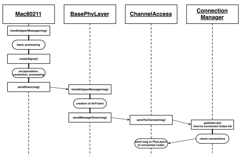
5.2 MiXiM physical layer functionality diagram . . . 51

5.3 MiXiM physical layer transmission flow diagram . . . 52

5.4 MiXiM reception functionality blocks . . . 54

5.5 802.11b and 802.11p PER curves at their lowest bit rates (1 and 3Mbps) . 55 6.1 MiXiM Decider - enhancements made to enable Frame Capture . . . 60

6.2 Comparison of the approximation function with the sampled function for BPSK (code rate 1/2) from Figure 2.13. . . 62

6.3 Validation experiment setup . . . 65

6.4 Required SNR for Frame Capture where strongest frame arrives first . . . 65

6.5 Comparison of Frame Capture experimental results, and the estimated results based on our implementation . . . 66

6.6 Frame Capture validation simulation results . . . 68

LIST OF FIGURES LIST OF FIGURES

7.2 The relationship between high node density and the hidden terminal

prob-lem. (S = Sender, R = Receiver, Q = Quiet, H = Hidden) . . . 71

7.3 Collision probability for single-lane scenarios . . . 78

7.4 Beacon success probabilities for th singe-lane scenarios. . . 79

7.5 Capture Factor for the single-lane scenarios . . . 81

7.6 Collision probability for single- and multi-lane (4 lanes) scenarios . . . 82

7.7 Beacon success probability comparison for the multi lane scenarios, all with 802.11p bit error calculations. . . 83

7.8 Capture Factor for the multi-lane scenarios. . . 84

7.9 Collision probability in the scenarios without hidden terminals . . . 86

7.10 Beacon success probability in the scenario without hidden terminal colli-sions. The upper two lines belong to the single-lane scenarios. . . 87

List of Tables

2.1 801.11a data rates and modulations / coding rates [1] . . . 23

3.1 802.11a and 802.11p PHY values [2] . . . 33

4.1 Frame Capture scenarios (data rate of 6 Mbps). These timing relations and results are for Atheros chipsets [3]. The experiments were performed with 802.11a. . . 39

4.2 Bit Error Rate calculation methods in various simulators . . . 43

7.1 Frame Capture simulation scenarios . . . 89

7.2 Simulation scenarios (numbers indicate # repetitions) . . . 89

1

Introduction

Nowadays, mobility and transport have become vital aspects of our society. Almost everybody has a car parked in front of their house or in their garage, which is used everyday - to get to work, to bring kids to school and pick them up, to visit family and friends, to buy groceries. . . these are just a few typical examples of how much we have gotten used and attached to our increased mobility and the convenience of owning a car. It is not even a luxury anymore; everybody has a car these days. With an increasing economy, both goods and people tend to move around a lot more and a lot faster than before, and the infrastructures we need to support that mobility are always expanding. But even though the infrastructure expands, it happens often that its capacity is not sufficient.

The traffic density on the Dutch highways is enormous, not just around the big cities, and on average working days there are over 200 km of traffic jams. This is about 4% of the entire Dutch highways network. Peaks in congestion due to weather conditions can rise up to 800 kilometers. The Dutch Ministry of Transport, Public Works and Water Management calculated that the annual economical damage because of traffic jams was between 2,8 and 3,6 billion euros in 2008. This was an increase of 7 percent compared to 2007, and even a 78 percent increase compared to 2000 [4]. These costs include both direct and indirect economical damage like extra fuel usage, the implied environmental footprint and commuters arriving late at work which causes companies to lose time and money. This does not only apply to the Dutch highways however, all growing societies around the globe suffer from heavy traffic congestion at peak hours.

1.1. PROBLEM STATEMENT CHAPTER 1. INTRODUCTION

carpooling) and in the Netherlands a system calledrekeningrijdenor ’billed driving’ has been proposed to distribute the infrastructure maintenance costs more evenly over the people who actually use it. However, none of these solutions actually try to increase the capacity that the roads in terms of ’passing vehicles per hour’ can sustain.

Vehicular networks try to fill that gap. By creating networks between vehicles, all users of the roads could have increased knowledge about the ’state’ of the road, the current amount of traffic and the speed at which the traffic on it travels. This information can then be used to increase the safety on the roads and the capacity, leading to less traffic congestion, reduced emissions and reduced costs.

This research does not cover the entire challenge of how vehicular networks can make our lives a bit easier, but merely a few of the aspects of it; we look at some of the challenges presented when simulating vehicular networks. Many application protocols and systems that are to be used in vehicular networks must of course be tested first, at different stages during their development. Simulation of these applications and protocols is an important step in this process. We can learn a lot about the expected behavior and find out how things would function and whether they are scalable without imple-menting all functionality in real cars. Also, simulations reduce the need for testing the behavior on circuits or blocking stretches of the highway, which is of course an expensive undertaking.

1.1

Problem statement

This thesis thus focuses mainly on the simulation of the physical layer in vehicular net-works. We give special attention to one problem in particular: Frame Capture. Frame Capture happens when two nodes try to send a frame to a third one at the same time and at the same frequency, i.e. when a collision occurs. Under some circumstances (de-pending on the signal to noise ratio’s and the arrival times of both) the receiver is able tocapture one of both frames, instead of losing them both because of the collision. This became the first important question that we tried to answer: How does Frame Capture work exactly? We looked at the knowledge that was already available and performed a literature study on three topics: basic IEEE 802.11 networks, the typical IEEE 802.11 physical layers and on Frame Capture. We looked specifically at the 802.11a and 802.11p physical layers because they are both based on Orthogonal Frequency Division Multi-plexing (OFDM). As can be read later in Chapter 3.4, IEEE 802.11p is the variety that is used for vehicular networks, which makes it the most important physical layer for us. Based on that literature study, the following observations came to the surface:

• Frame Capture behaves differently on chipsets of different manufacturers [5, 6, 3].

CHAPTER 1. INTRODUCTION 1.2. RESEARCH QUESTIONS

Much more information about IEEE 802.11 and Frame Capture will be presented later in this thesis. These two observations and the literature study also lead to my main problem statements:

• Frame Capture is probably important for vehicular networks. However it is still unknown to which extent.

• IEEE 802.11p, the standard for vehicular networking, is poorly sup-ported by almost all wireless network simulators. There are quite a few network simulators around and some of them also support wireless communication protocols. However, the standard that will be used for vehicular networking, IEEE 802.11p [7], is relatively new and is not yet fully supported, not by any simulator currently available.

• Frame Capture, although interesting, is not accounted for in the wire-less network simulator that our research group normally uses (which is MiXiM [8], a wireless network simulator built within the OMNeT++ framework [9]). Frame Capture is at best poorly implemented and in all situa-tions poorly documented.

Also, when answering these questions regarding to Frame Capture and looking into our wireless network simulator, another problem arose:

• MiXiM does not provide bit-error estimation functions in its physical layer implementation for 802.11a or 802.11p. The functionality present is only for 802.11b, which is fundamentally different [10].

1.2

Research questions

Based on these problems, the following research questions were formulated:

1. How can Frame Capture behavior in an IEEE 802.11p vehicular network be modeled?

How does Frame Capture behave in 802.11a networks? Will that be much different from 802.11p? It is necessary to account for the different behavior types found in different chipsets.

2. How can the current IEEE 802.11 physical layer implementation in MiXiM be improved?

Which changes are needed to facilitate IEEE 802.11p communication and what important factors are not yet considered? In these changes to the physical layer, Frame Capture must also be considered.

3. How does Frame Capture influence IEEE 802.11p network performance in a vehicular environment?

1.3. OUTLINE CHAPTER 1. INTRODUCTION

Frame Capture have a positive effect on the network throughput in a broadcasting environment (i.e. a network where most traffic is broadcast traffic)?

4. What is the relationship between the hidden terminal problem and Frame Capture?

Does Frame Capture still occur if the hidden terminal problem were not present?

We try to answer the last two questions by performing simulations with the imple-mentation resulting from the first two and in doing so, we tried to solve the problems mentioned and provide more insight in Frame Capture and its relationship to vehicular networks.

1.3

Outline

This thesis is structured as follows: in Chapter 2 we first provide basic background information about IEEE 802.11 wireless networks in general, look at the hidden terminal problem and at the reasons that collisions can occur in a wireless network. We then look at the physical layer by examining the inner workings of OFDM, the technology at the core of the physical layer of 802.11a and 802.11p. After this general introduction, Chapter 3 discusses vehicular networks. We look at what makes them different from the normal wireless networks, what their potential applications are and where the great challenges lie when dealing with vehicular networks. In Chapter 4 we discuss Frame Capture, what it is exactly, how and when it happens and we try to illustrate this with figures found in literature about the exact scenarios at which Frame Capture occurs. We also analyze the impact of Frame Capture on vehicular networks. Chapter 5 then provides more insight in our wireless network simulator and especially its physical layer - how it works and what we need to change to implement Frame Capture.

2

IEEE 802.11 Wireless Networks

In this chapter we discuss various aspects of the 802.11 wireless networking family and the required specifics about the MAC and physical layers. We focus on the modulation and multiplexing techniques of 802.11a and 802.11p (OFDM). Readers already familiar with wireless networking can probably skip Sections 2.1 and 2.2 about the MAC layer, CSMA/CA and the hidden terminal problem.

2.1

Basics

2.2. MEDIUM ACCESS CONTROL CHAPTER 2. IEEE 802.11 802 Overview and architecture 802.1

Management 802.2 Logical Link Control (LLC)

802.3 MAC 802.5 MAC 802.3 802.5 PHY PHY 802.11 MAC 802.11 FHSS PHY 802.11 DSSS PHY 802.11 OFDM PHY 802.11 HR/DSSS 802.11 ERP PHY

Figure 2.1: The IEEE 802 family (Copied from [1], Figure 2-1).

2.2

Medium Access Control

Because the wireless medium is a lot different from the wired medium used in for example 802.3 (Ethernet), a new MAC layer needs to be defined to successfully mitigate problems such as interference, collisions and the increased security vulnerability. Therefore, an adapted access scheme is used in this MAC layer: Carrier Sense Multiple Access with Collision Avoidance (CSMA/CA). This access scheme counters at least some of these problems. It contains a few different coordination functions, among them the Distributed Coordination Function (DCF). This is the most common one, and is the one relevant to discuss in this thesis.

The DCF organizes the access to the medium according to a set of basic rules.

• If the station wants to send a frame, it first senses the channel to see if somebody else is sending (this is called carrier sensing). If the medium is idle during a predefined period of time called the Distributed Inter-Frame Space (DIFS), the node can start sending right away. If the medium is busy, the station defers from sending and waits until the medium becomes available again. After the medium has become available, it again senses the medium for a DIFS.

• If during this second DIFS the medium remains idle, the station enters a so-called contention window or backoff window. This is a time window divided in slots. The window size (in number of slots) depends on previous transmissions, but has a minimum and maximum defined by the standard. In 802.11p the contention window size is between 15 and 1023 slots and always increments in powers of 2. Every slot has a fixed duration, it depends on the physical layer what the exact length is (in 802.11p it is 16µs). The station randomly chooses a number of slots (within the contention window), that is the number of time slots it will wait before it actually starts trying to transmit. This means that if two stations were both waiting for a transmission to end, they will not start transmitting directly after the DIFS (and generate a collision). After picking a random number of (say n) slots thebackoff timer starts counting down from n to zero, when it reaches zero the station can transmit.

CHAPTER 2. IEEE 802.11 2.2. MEDIUM ACCESS CONTROL

Data

Defer access

SIFS

ACK

DIFS

Data

Contention window

Backoff after defer

Sending station

Receiving station

Other stations

Figure 2.2: The IEEE 802 DCF. (Based on [12], Figure 3-7)

because another station was also waiting and picked a random number smaller than its own, it freezes the backoff timer. Then, after that transmission and a DIFS of idle time on the medium, it does not pick a random number again but merely restarts the backoff timer. This means that a station which had to wait the first round has a higher probability of gaining first access to the medium in the subsequent rounds.

• If the backoff timer reaches zero, the station transmits. If then the transmis-sion fails (i.e. no Acknowledgement (ACK) is received), it doubles the contention window size and tries again. This means that when the number of nodes (and col-lisions) in the network increases, stations automatically start waiting longer and the algorithm remains stable.

• If a station needs to transmit a frame that, in the algorithm, logically follows the just transmitted frame (such as an ACK frame to indicate correct reception, or a new data frame if the entire frame is being fragmented), the station does not have to wait for a DIFS period. Instead, it can start transmitting after a Short Inter-Frame Space (SIFS), this guarantees that no other station that is not involved in the current transmission can seize the medium before it is completed. In this way multiple Inter-Frame Spaces are defined for frames with different priorities.

In Figure 2.2 part of the algorithm is shown in action. A sending station starts trans-mitting a data packet after waiting a DIFS, the receiving station replies after waiting a SIFS with an ACK, and after a DIFS and a random backoff period another station that also wanted to send a frame can start transmitting.

2.2. MEDIUM ACCESS CONTROL CHAPTER 2. IEEE 802.11

in Figure 2.3. This happens when two nodes both want to transmit but cannot hear each other. This can happen for many different reasons; for example when there is an obstacle in between, or because they are simply too far apart. It does create possible collision scenarios though, because in network situations like the one in Figure 2.3 the carrier sensing mechanism alone is not enough. If either node A or C starts transmitting to B (because it thinks the channel is idle) while the other node is also transmitting, either to B or to another node in the network, their transmissions will overlap spatially at node B, causing B to perceive a collision of two signals.

A B C

Figure 2.3: Simplified visualization of the hidden terminal problem.

CHAPTER 2. IEEE 802.11 2.3. OFDM

Figure 2.4: Orthogonality of subcarriers in the frequency domain (Copied from [13]).

2.3

Orthogonal Frequency Division Multiplexing

2.3.1 Introduction

IEEE 802.11p uses a physical layer similar to 802.11a with OFDM as the primary mul-tiplexing technique. In this section we will look into OFDM and describe how it works, so that the concept is clear in the later chapters about 802.11p and Frame Capture (Chapters 3.4 and 4).

Normal (single-carrier) modulation techniques use the whole channel and modulate data onto a signal at a high rate, with one symbol occupying the entire bandwidth for a

very short time. OFDM however divides (or multiplexes) the channel in many small

subcarriers and every subcarrier is modulated at a much lower rate. In order not to waste too much bandwidth on guard bands between these subcarriers, their frequencies are chosen in a such a way to createorthogonality; without spacing between the carriers they do not interfere with each other. This of course greatly improves the channel efficiency. In the power spectrum from Figure 2.4 we clearly see that at the peak of every subcarrier all other subcarriers are zero, i.e. at that frequency the other subcarriers do not contribute any energy to the signal. The orthogonality is crucial to OFDM, if subcarriers are not chosen orthogonal to each other, they will overlap and interfere significantly.

2.3. OFDM CHAPTER 2. IEEE 802.11

I Q

(a) BPSK constellation

diagram

(b) Example of BPSK modula-tion (Based on [14], Figure 9-15)

I Q

A

φ

(c) Explanation of the con-stellation

Figure 2.5: BPSK and QAM constellations

2.3.2 OFDM mathematics

In order to explain how these orthogonal subcarriers are exactly generated, we need to look a little bit into the mathematics behind OFDM. Let’s first look at OFDM in the time domain:

An OFDM subcarrier is a normal sine wave at a certain frequency, modulated with the data. As said before the frequency does not change, only the phase and amplitude can be modulated. Typical modulation schemes that achieve this are Binary Phase Shift Keying (BPSK), Quaternary Phase Shift Keying (QPSK) or Quadrature Amplitude Modulation (QAM). These modulations can be described in the complex plane as ’constellations’ of points, where each point is the same sine wave but at a different phase and/or amplitude, and each point encodes a number of bits. This is illustrated in Figure 2.5. If the number of points in the constellation increases, more bits can be mapped onto each point. In Figure 2.5(a) for example, there are 2 points and only a 0 and a 1 can be mapped on both points. In Figure 2.5(c) each point in the constellation represents 4 bits, which means that there are 24 = 16 points in total. In the complex field, a vector can be drawn from the origin to the point: the angle that the vector makes with the x-axis is the phase (ranging from 0 to 360◦), and the length of the vector is the amplitude.

The desired orthogonality is created in two steps: carefully choosing the subcarrier frequencies and, after summing all the subcarriers, calculating the convolution (a type of integral transform ) of the summed signal with a so-called rectangular window. A rectangular window is quite a simple signal: it is 1 between−T₂ and T₂, 1₂ at the borders and 0 otherwise. The rectangular window used in OFDM is 1 between 0 and T (shown in Equation 2.1).

rect(t) = 





0 ift <0 ort > T

1 ift >0 andt < T

1

2 ift= 0 or t=T

(2.1)

CHAPTER 2. IEEE 802.11 2.3. OFDM

R∞

−∞rect(t)·e

−i2πf t_dt= sin(πf)

πf = sinc(f)

(a) Fourier-transform of rectangular window (b) The resulting spectrum

Figure 2.6: The Fourier transform of the rectangular pulse

this rectangular pulse, we see that the spectrum of this rectangular is a sinc function (as in Figure 2.6(a)).

Asinc function looks exactly like the carriers in Figure 2.4, it has a peak at one specific frequency and is 0 at the center frequencies of the adjacent subcarriers, or in the time domain, at the nonzero integer values of t. This means that the rectangular pulse in

the time domain looks like a sinc function in the frequency domain. Any signal that

is convoluted with a rectangular pulse of the right width looks exactly like a subcarrier as in Figure 2.4. The width of the pulse defines the distance between the peaks in the resulting spectrum. This is valid with only one subcarrier, but by choosing the other subcarriers just the right way (explanation in Appendix B), summing them and after that calculating the convolution with the rectangular window creates an OFDM signal (convolution in the time domain is equal to multiplication in the frequency domain) where every subcarrier has one peak as in Figure 2.6(b), and is zero on the frequencies of all the adjacent peaks. This allows very closely placed subcarriers, increasing the spectral efficiency of the signal. The frequency difference between the subcarriers needs to be

fc= _T1. As an example, T in 802.11a is 3.2µs, this corresponds to 1/3.2·10−6 = 312.5 kHz subcarrier spacing.

All the above would result in a spectrum (for 802.11) that looks like Figure 2.7. At the gaps in the spectrum are special pilot carriers, used for time and frequency synchroniza-tion purposes.

Carrier number Center

frequency

-25 -20 -15 -10 -5 0 5 10 15 20 25

Figure 2.7: 802.11 OFDM channel structure (Copied from [1], Figure 13-8).

2.3. OFDM CHAPTER 2. IEEE 802.11

of the subcarriers themselves is low, but because OFDM uses many subcarriers the total data rate is equal to a single-carrier system.

2.3.3 Preamble detection

At the physical layer of 802.11a and 802.11p, Physical Layer Convergence Protocol (PLCP) handles the formatting of the frame. The PLCP preamble is an important phase of that frame and the reception process in general. A receiver goes through the following steps during the preamble:

1. Detection and measurement of the signal power level; this has to be greater than or equal to RXSens, which is the receiver’s minimum coding & demodulation sensitivity. Any signals with a power level below this threshold will be considered as noise. RXSens for Atheros chipsets is around -91 dBm [15].

2. Automatic Gain Control (AGC) during which it sets the signal gain to a level appropriate for the received signal power. This is necessary to have the signal arrive at the receiver circuitry with always the same power level.

3. Frequency synchronization using a Phase-Locked Loop (PLL) (see also Ch. 7 & 8 of [14]).

4. Timing synchronization [15].

A visualization of the PLCP frame and preamble is given in Figure 2.8. Note that the time values mentioned in Figure 2.8(b) apply to 802.11a. The preamble consists of 10 small predefined symbols followed by two large ones. The short ones are used for AGC and frequency synchronization and the two long ones are used for fine-tuning. In general the rule applies that the longer the preamble is, the better the receiver can estimate the channel and the better the receiver can lock to the signal. [1, 16].

2.3.4 Guard times, coding and forward error correction

There are many types of interference and disturbances which can disrupt or destroy a signal in the wireless medium. Two of them are Inter-Symbol Interference (ISI) and Inter-Carrier Interference (ICI). ISI occurs when two subsequent symbols interfere with each other; this is caused by multipath propagation or frequency delays which disrupt the receiver’s timing synchronization. ICI is caused when (perhaps in a narrow part of the frequency band) the carrier frequency shifts a little bit. This disrupts the orthogonality of the subcarriers and causes energy of one subcarrier to leak into another. This can be caused for example by Doppler shift, which can be a serious problem in OFDM.

To counter ISI, every OFDM symbol starts with aguard time; this is a small portion of

the symbol time. The symbol time is divided in the guard time and the Fast Fourier

CHAPTER 2. IEEE 802.11 2.3. OFDM

(a) PLCP Frame Layout

(b) PLCP Preamble (and first data symbols)

Figure 2.8: PLCP Frame and Preamble for 802.11a (Copied from [1], Figure 13-14

and 13-15)

multipath delay can cause various ’copies’ of the original symbol to arrive at the receiver, also called different signal components. These components are generated by reflection of the signal against buildings, metal structures and other big objects. The Line Of Sight (LOS) component is the part of the signal that arrives directly at the receiver, and usually at various delays one or more multipath components show up, at a lower amplitude than the LOS component. If because of multipath delay a part of the previous symbol arrives during the guard time, this does not interfere with the symbol itself. This is only true however if the guard time is chosen such that it is bigger than the biggest reasonably expected multipath delay. More about multipath delay and multipath fading can be found in Appendix A and in Chapter 10 of [1].

The multipath components do not cause variations in the frequency, so the orthogonality is still preserved. However to preserve the orthogonality of the signal the receiver must have an integer number of cycles in the FFT integration time. This integer number is needed because the FFT works with discrete samples drawn from the signal, not the original signal itself. If in the FFT integration time there is not an entire cycle (360◦ in the complex field) or an integer multiple of that, the sampling stops at some signal value and the next sampled value (belonging to the next symbol) will differ greatly. This results in discontinuities in the signal, and this changes the perceived frequency of the subcarrier. This in turn destroys the orthogonality of the signal [1].

2.3. OFDM CHAPTER 2. IEEE 802.11

Guard time FFT integration time

Subcarrier 1

Subcarrier 2

Previous symbol

Delay

Figure 2.9: Cyclic prefix extension (Based on [1], Figure 13-6)

during the guard time (see Figure 2.9). This is called cyclic prefix extension. Also, in situations where there is no LOS component, the OFDM receiver could in the best case still figure out based on a multipath component what the original symbol was.

In order to further increase robustness of the signal, a typical OFDM transmitter also adds coding to the data. This is strictly not part of OFDM, but very commonly used in combination with it. The coding enables Forward Error Correction (FEC) at the receiver; with FEC a receiver can detect and correct errors without requiring retransmission. Coding works as follows: the encoder expands the original data bitstream, thereby

adding redundancy. How much redundancy is added is determined by the coding rate,

for 802.11 this varies between 1/2 and 3/4. A coding rate of 1/2 means that every original data bit is replaced with 2 coded bits. There are many different coding algorithms which vary in complexity, the one that is used in 802.11 is a so-called convolutional encoder. A convolutional encoder works on a continuous stream of bits; it takes m bits as input

and produces n output bits, where the coding rate is m/n. It uses a transformation

function that has a shift register with the last 7 input bits. On every step it computes

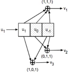
noutput bits based on the 7 bits in the register, andm bits in the register are replaced with new input bits. An example of a small convolutional encoder (with only 3 bits in the register) is given in Figure 2.10. In this encoder the values in the registers are summed to create the various output bits. The way the register bits are combined (or thegenerator polynomials for the various output bits) is critical to the error-correction properties of the encoder, they vary depending on the coding rate and the number of registers (orconstraint length).

CHAPTER 2. IEEE 802.11 2.3. OFDM

Figure 2.10: An example of a convolutional encoder with 1 input bit, 3 output bits and

3 bits in the register. Please note that this is just an example of an encoder, the real encoder used for 802.11 is visualized in Figure 2.12.

bit errors occur, the Viterbi algorithm outputs the most likely sequence of data bits, depending on the encoding and the occurrences of the bit errors. [1, 17]

One last smart step that the OFDM transmitter performs is interleaving: it spreads the coded bits over all subcarriers (1 bit at carrier 1, next bit at carrier 2, next at carrier 3 and so on), so that in the case of narrowband interference the bit errors are spread over the input bit stream. The probability of multiple bit errors close together (after de-interleaving) decreases, and if the decoded bits have errors, they can be more easily be corrected by Forward Error Correction because of the larger distance between errors. The receiver thus has a higher probability of finding the right data bits based on the encoded bits.

2.3.5 Strengths and weaknesses of OFDM

The multiplexing scheme used in OFDM has a few significant advantages over the single-carrier schemes used for instance in 802.11b. All the small subsingle-carriers together generate a very flat, evenly distributed spectrum. The spectral efficiency is high; subcarriers are orthogonal to each other and placed very closely together. The various protection mech-anisms make the signal very robust to narrowband interference and multipath fading, and ISI is effectively countered by the cyclic prefix extension (given that the delays are not much longer than the guard time). Also, the efficiency loss caused by this cyclic prefix is acceptable because of the low symbol rate. Another advantage is that OFDM can be implemented in transmitters and receivers using relatively simple components, no advanced equalization circuits are needed.

2.3. OFDM CHAPTER 2. IEEE 802.11 Transmitter FEC (Convolution encoder) Interleaving, mapping, and pilot insertion IFFT Guard interval insertion I-Q modulation HPA Pilot remove, deinterleaving, and demapping FFT Guard interval removal I-Q demodulation

LNA AGC FEC

decoder

Receiver

Figure 2.11: An OFDM transceiver block diagram (Copied from [1], Figure 13-17)

This increases the complexity at the transmitter, since practical Power Amplifiers (PA’s) have a range at which they are linear (i.e. linearly amplifying the signal), and another part (near saturation) where they are non-linear. If the amplification is non-linear, this changes the form of the received signal at the receiver and thus increases bit errors [18, 19].

2.3.6 OFDM transmission and reception blocks

This section shows transmitter and receiver blocks for typical OFDM chipsets, and explains some of the steps that a transmitter goes through when transmitting data.

When looking at Figure 2.11, an OFDM transmitter does the following steps when transmitting (note that some of these steps are specific to 802.11) [1]:

1. Transmission rate selection. This depends on the channel conditions but is chipset-implementation dependent. The rate does dictate however which modulation is used and which coding rate. Together the modulation and coding rate determine how many bits are transmitted per symbol. Table 2.1 contains an overview of the used combinations.

2. Transmission of the PLCP preamble (at a fixed rate of 1 Mbps), these are a few long and short symbols to train the receiver and enable frequency synchronization.

3. Transmission of the PLCP header, also at 1 Mbps, which contains info about the frame that is about to be transmitted (frame length, encoding, transmission rate that will be used).

CHAPTER 2. IEEE 802.11 2.4. BER CALCULATIONS

5. Division of the coded bits into blocks (depending on the number of bits per OFDM symbol) to perform the interleaving process.

6. Pilot subcarrier insertion and using the Inverse Fast Fourier Transform (IFFT) generate the data signals.

7. Modulation of the subcarriers with the data signals using I-Q modulation. This modulation type is how QAM and QPSK signals are generated, for more informa-tion readers are referred to Chapters 9-5 and 9-6 of [14].

8. Amplification of the entire signal in a High-Power Amplifier (HPA) for transmission over the antenna.

When a frame is being received, the signal is first amplified using a Low-Noise Amplifier (LNA), and AGC is applied to get the signal to the (standard) power levels needed for demodulation. The rest of the reception process is basically the reverse of the sending process, as can be seen in Figure 2.11.

Table 2.1: 801.11a data rates and modulations / coding rates [1]

Transmission rate (Mbps) Modulation Coding rate Coded bits per carrier Coded bits per symbol

Data bits per symbol

6 BPSK 1/2 1 48 24

9 BPSK 3/4 1 48 36

12 QPSK 1/2 2 96 48

18 QPSK 3/4 2 96 72

24 16-QAM 1/2 4 192 96

36 16-QAM 3/4 4 192 144

48 64-QAM 2/3 6 288 192

54 64-QAM 3/4 6 288 216

2.4

Bit Error Rate Calculations

2.4. BER CALCULATIONS CHAPTER 2. IEEE 802.11

The aim is to use these bit error calculations in our implementation of 802.11p in the physical layer of our simulator. As known and described in Chapter 2.3, OFDM uses BPSK, QPSK and QAM as modulation techniques for various bit rates. The symbol error probability can be intuitively understood as the probability that noise or interference shifts the constellation point (see Chapter 2.3.2) so much that it ends up in another part of the constellation. The symbol error probability for BPSK [20] is shown in Equation 2.2.

Ps=Q r

2Eav

N0

(2.2)

In Equation 2.2, Eav/N0 is the effective Signal to Noise Ratio (SNR) per bit. Q(x)

is the Q-function, which is the inverse of the normal cumulative distribution function of a Gaussian distribution (i.e. the integral that calculates the surface under the right tail).

Q(x) = 1

2(1−erf(

x

√

2)) (2.3)

erf(x) = √2

π

Z x

0

e−t2dt (2.4)

Since with BPSK there is only 1 bit per symbol, the symbol error probability is also

the bit error probability. The symbol error probability for M-ary QAM in an AWGN

channel is given in Equation 2.5.

PM = 1−(1−P√_M)2 (2.5)

P√

M = 2· 1− 1 √ M ! ·Q r 3

M −1

Eav

N0

!

(2.6)

These formulas calculate the symbol error probability. The QAM constellation is Gray coded, which means that all adjacent QAM symbols are chosen such that they differ only in 1 bit [21]. Therefore if a transmitted symbol shifts to an adjacent one in the constellation, only 1 bit error occurs [20, 22], if the adjacent symbol represented a bit sequence that differed in more than 1 place, we would also have more than one bit error. That results in the following formula for the bit error probability:

Pb ≈ 1

log₂M ·PM (2.7)

CHAPTER 2. IEEE 802.11 2.4. BER CALCULATIONS

T

T

T

T

T

T

+ + + +

+ +

+

+ output 1

output 2 input

Figure 2.12: The convolutional encoder used in 802.11a and p. It has generator

poly-nomials g0 = 1338 = 9110= 10110112 and g1 = 1718= 12110= 11110012. (Copied from

[22], Figure 2.8)

a few other elements to take into account. First: theEav/N0 value (the effective SNR)

needs to be lowered, because not all the transmitted energy is stored in the information bits of the signal. A large cyclic prefix was added to counter ISI and ICI. The correct value forEav/N0 is given in Equations 2.8 and 2.9.

Eav

N0

= α·_P C

I+N (2.8)

α= TIF F T

TIF F T +Tg

= 6.4µs

6.4µs−1.6µs = 0.8 (2.9)

HereTIF F T is the Inverse Fast Fourier Transform period, equal to the symbol time, and

Tg is the guard time, equal to the cyclic prefix length. C is the packet energy level and P

I +N is the sum of all interfering signals and noise. As we can see, all SNR values should be multiplied by 0.8 in and OFDM channel since 20% of the time there is no information transmitted [20].

Apart from this a normal 802.11a or p transceiver also performs coding and forward error correction on a signal. All input bits are encoded using a convolutional encoder with generator polynomials g0 = 1338 and g1 = 1718. This encoder is visualized in

Figure 2.12.

Since the input bit stream is interleaved (consecutive bits are spread among all sub-carriers), if a symbol error occurs the resulting bit errors are spread across the output bitstream. If they are separated enough, they can be corrected by the Viterbi decoder. We will not elaborate on all the details of error-correction here, they can be found in [23, 24].

Because of the error correction the packet error probability is not easily derived from the bit error probability. Instead, we can calculate an upper bound on the packet error probability, which is given by

2.4. BER CALCULATIONS CHAPTER 2. IEEE 802.11

P_um=

∞

X

d=df ree

αd·Pd (2.11)

Pd=            d P

k=d+1₂

d k

pk(1−p)d−k, d= odd

d P

k=d₂+1

d k

pk(1−p)d−k+1_{2 d/}d₂pd/2(1−p)d/2, d= even

(2.12)

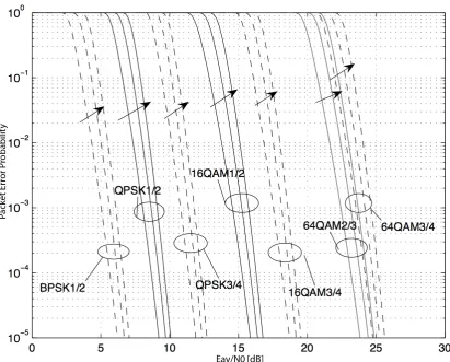
Here dfree is the minimal free distance of the convolutional code (10 in this case),αd is the total number of errors with weight d and Pd is the probability that such an error occurs [20, 25]. This is also further explained in Chapter 8-2 of [24]. All these formulas combined yield the numerical results shown in Figure 2.13.

From all the equations and formulas shown above, we can conclude that there are many factors involved when determining the success probability of a transmission. We tried to summarize this here:

• Modulation plays an important role. If there are many bits in one symbol, the

amount of noise or interference that a receiver can tolerate becomes less.

• Coding has a positive effect on the success probability in general. By adding a few redundant bits to the stream, bit errors can be corrected up to a certain point. This is complex mathematics though, we haven’t investigated all the details of error-correction coding.

• The transmission rate is derived directly from the modulation and the coding

rate. If a higher-order modulation is used that puts more bits in one symbol, the transmission rate increases. The coding rate defines how much redundancy is added and decreases the transmission rate, e.g. if a coding rate of 2/3 is used, one in every 3 bits is redundant, reducing the number of ’real’ information bits.

• As can be seen in Figure 2.13, the length of the frame also influences the success probability. If we assume an equal error probability for every (decoded) bit, the chance of having one error in a frame increases with packet length. However the channel has a so-calledchannel coherence time, which is the time that the channel is assumed constant by the receiver. Depending on the channel, a frame cannot be longer than a certain length, otherwise bit errors do start to increase. More about this can be read in Section 3.4.2 and [20].

CHAPTER 2. IEEE 802.11 2.4. BER CALCULATIONS

Figure 2.13: Numerical results for the packet error probabilities of all QAM variations

2.4. BER CALCULATIONS CHAPTER 2. IEEE 802.11

3

Vehicular Networks

This chapter discusses some of the basics about vehicular networks; why do we want them, what can they do for us and what do we need to take into consideration when designing a vehicular network?

3.1

Basics

Vehicular networks are networks between vehicles, other vehicles and in some cases roadside infrastructures. A vehicular network can enable a wide variety of applications, both user-oriented and safety- and vehicle-oriented. There is a lot of similar terminology describing the same concepts, a the most commonly found terms are [26]:

• Intelligent Transport Systems (ITS)

• Inter-Vehicle Communication (IVC)

• Vehicular Ad-Hoc Networks (VANETs)

• Vehicle to Vehicle (V2V) Communication

• Vehicle to Infrastructure (V2I) Communication

3.2. APPLICATIONS CHAPTER 3. VEHICULAR NETWORKS

and processing, access to larger (backbone) networks such as the internet and security features such as encryption key distribution. Both systems have many advantages: an ad-hoc network is easy to set up, can be deployed anywhere and is only present when there is traffic and is, up to a certain degree, very scalable, i.e. it does not depend on the capacity of the roadside infrastructure. There is a trade-off however, routing in an ad-hoc network is very hard and reliability depends greatly on the number of vehicles within range. If there are too few cars information might get lost, and if there are too many cars sophisticated algorithms are necessary to prevent the network from saturat-ing. Also, some applications such as regular internet connectivity are not possible with a pure ad-hoc network since the vehicles only communicate with each other. A V2I infrastructure is more costly to deploy, but mitigates many of the disadvantages found in ad-hoc networks.

3.2

Applications

A few examples of user-oriented applications are normal internet connectivity for drivers, instant messaging, automatically updating the maps of satellite navigation devices, au-tomated route planning and any internet-based personal entertainment as can be found in modern smartphones and tablets. However, the safety- and vehicle-oriented appli-cations of vehicular networks are a lot more interesting from an academic perspective. There are many examples:

• Cooperative Adaptive Cruise Control. Some car brands already have Adap-tive Cruise Control (ACC), a safety feature where the car measures the distance to the vehicle in front of it, and if that becomes too small (or decreases too fast), the car automatically starts braking, whether the driver is pushing the brakes or not. Cooperative Adaptive Cruise Control (CACC) achieves the same by letting the cars exchange messages when they brake, controlling and coordinating the longitudi-nal movement (and acceleration and deceleration) of an entire stream of vehicles. It has been proven that the response of a CACC system is much faster than its non-communicative ACC counterpart [27]. Note that CACC is not a pure vehicle safety application - it is also about comfort for the driver and about improving the efficiency of the traffic on the road.

CHAPTER 3. VEHICULAR NETWORKS 3.3. CHALLENGES

• Traffic flow optimization. If vehicles on the highway would be able to coordinate their speed with all other vehicles around them using V2V communication and make intelligent decisions regarding their speed, not just based on the 10 vehicles in front of the driver (what the driver can see), but based on all vehicles in the coming few kilometers, the flow of traffic would be a lot smoother, resulting in increased capacity of the road network, fewer traffic jams and major decrease of economical damage because of traffic congestion.

Our research group focuses mostly on the safety- and efficiency applications of vehicular networks. It can be easily understood that for safety-critical applications direct com-munication between vehicles provides many advantages over relaying traffic via roadside units, so for these kind of applications at least some form of ad-hoc networking must be present. This thesis therefore also focuses on the ad-hoc nature of vehicular networks. Ad-hoc network connectivity does not exclude V2I communication however, but we fo-cus on the former. The standard (to be disfo-cussed in Chapter 3.4) however accounts for both.

3.3

Challenges

In a vehicular networking environment, two typical scenarios need to be considered primarily: urban and highway environments. In both cases the ’ad-hoc’ characteristic of the network is quite extreme. On a highway vehicles don’t always stay close to each other for a long time, and all vehicles travel in the same direction (if assumed that the vehicles traveling in the opposite direction form a separate network), but at every fork or exit nodes can enter or leave the network. It is thus incorrect to assume that a node in the network is still there if it was 60 seconds ago. This is even more true in an urban environment, where the vehicles have an even higher degree of freedom of movement [29, 30].

In such an environment, it is absolutely impossible to use a standard 802.11a, b or g wireless (ad-hoc) network. Tasks like authentication, updating routing tables and sending packets to other nodes are very unreliable because the network topology changes

too much in very short periods of time. Typical Access Point (AP) scanning costs

3.4. IEEE 802.11P CHAPTER 3. VEHICULAR NETWORKS

Apart from the limitations from the MAC layer such as authentication, the physical layers from a standard Wireless Local Area Network (WLAN) are also not designed to handle that much movement. One of the normal WLAN variations, 802.11a, uses OFDM which is very sensitive to Doppler-shift (see also Chapter 2.3.5). If no effective countermeasures are taken, Doppler shift will significantly influence the efficiency and throughput of the vehicular network [32, 33]. Altogether many factors need to be con-sidered in a vehicular network that are not that relevant in normal 802.11 infrastructure or ad-hoc networks.

3.4

IEEE 802.11p

IEEE 802.11p is the amendment to the 802.11 wireless networking family that will facili-tate vehicular communication and provide solutions to many of the problems mentioned above. It specifies many of the needed adaptations, one of the main concepts they intro-duced is called Wireless Access in Vehicular Environments (WAVE). The standard has only recently been published (July 2010) and has been under development since 2006. The amendment only specifies changes at the MAC- and physical layers, higher layer protocols such as TCP and IP are considered out of the scope of the 802.11 standard. Considering the MAC layer, a Station (STA) can operate in WAVE mode, and when it does it can send messages to any other STA in WAVE mode with a valid MAC address, including group addresses, without first joining a Basic Service Set (BSS). If communi-cation with a Distribution System (DS), a fixed road-side network is necessary, stations can also join a WAVE Basic Service Set (WBSS). Authentication or association is not required in WAVE mode, only the first step (joining the BSS) has to be performed. After that, data is sent directly to the DS [7].

3.4.1 Physical layer

The changes to the physical layer in 802.11p are a lot more interesting to us. The frequency band at which 802.11p will operate is in the 5.9 GHz ITS channel in the US, this band has been designated by the Federal Communications Commission (FCC) for use by Intelligent Transport Systems. The European telecommunications authority, or Conf´erence Europ´eenne des administrations des Postes et des T´el´ecommunications (CEPT), has designated a similar frequency spectrum after extensive studies [34, 35].

CHAPTER 3. VEHICULAR NETWORKS 3.4. IEEE 802.11P

spread decreases (due to the smaller frequency bandwidth), inter-symbol interference is also decreased due to the longer guard times. These doubled parameters in the time domain halve the effective data rate (3 to 27 Mbps against 6 to 54 in 802.11a) [36]. The standard also specifies more stringent Adjacent Channel Rejection (ACR) requirements, because the guard bands between channels are smaller. Table 3.1 contains a comparison of various 802.11a and p Physical Layer (PHY) parameters.

Table 3.1: 802.11a and 802.11p PHY values [2]

Parameter 802.11p 802.11a

Channel bandwidth 10 MHz 20 MHz

Data rates 3 to 27 Mbps 6 to 54 Mbps

Slot time 16 µs 9 µs

SIFS time 32 µs 16 µs

Preamble length 32 µs 20 µs

PLCP header length 8 µs 4 µs

Air propagation time <4 µs << 1µs

CWmin 15 15

CWmax 1023 1023

3.4.2 Effects of changes at the physical layer

The changes made to the physical layer have been chosen such that communication is still possible using OFDM, in spite of the increased amount of movement, Doppler shift and the challenging channel characteristics. The typical rms delay spread for a non-LOS signal component can be up to 400ns [37], this can more or less be interpreted as (quadratic mean of) the time difference between the LOS component and the last non-LOS component. The guard time is 1.6µs, so the guard time is enough to eliminate ISI. However, according to [20], some efforts are still needed to protect the physical layer against the short channel coherence time and the increased amount of mobility. If we assume a maximum speed of 500 km/h, the maximum Doppler spread will be 2.7 KHz and that indicates a channel coherence time of 157µs. A frame that is transmitted must not be longer ’on the air’ than this period, or the training symbols at the start of a frame will not be long enough and the signal can become too distorted. The frame size that this relates to depends on the bitrate, but this is only 471 bits for the lowest data rate (3Mbps·157µs) [38].

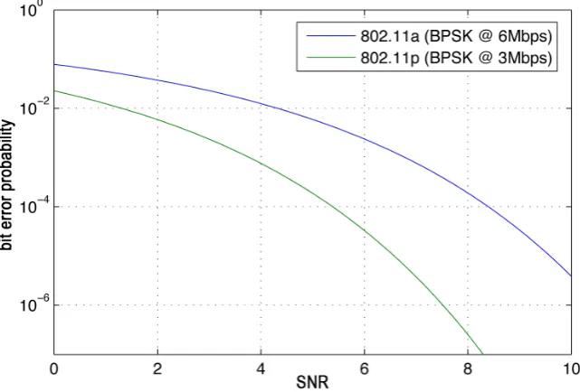
Since the bit error probability (in an AWGN channel) of a communication system relies only on the SNR per bit or Eb/N0 (Chapter 5-2-1 of [24]) and not on any other

3.4. IEEE 802.11P CHAPTER 3. VEHICULAR NETWORKS

Figure 3.1: BER curves for uncoded BPSK with 802.11a and 802.11p.

symbol and doubled energy per bit (Equation 2.2. The resulting difference in (uncoded) bit error probabilities is shown in Figure 3.1, we can see that a doubled Eb/N0 value

implies a significantly lower bit error rate. The difference (in energy per bit) between both physical layers that is needed to achieve the same uncoded Bit Error Rate (BER) is exactly 3 dB.

The error-correction coding is exactly the same in 802.11p as in 802.11a, it introduces another change in the energy per bit and in the final bit error probability (Chapter 1.9 of [39]). While coded and uncoded channels are hard to compare, using a convolutional or block code results in a coding gain of a few dB that is independent of the SNR or

Eb/N0 [39, 23]. We thus expect the resulting coded BER curve to show a similar shift

4

Frame Capture

Now that we have covered all the basics about 802.11 communication and the challenges with vehicular networks, we focus on the phenomenon that we try to research with this thesis: Frame Capture. This Chapter covers all aspects of it; what it is, when and how it occurs and what its potential impact is on vehicular networks.

4.1

What is Frame Capture

Frame Capture occurs under some conditions when two transmissions overlap both spa-tially and temporally. When a receiver detects two frames at the same time this is generally regarded as a collision - if two sources send an electromagnetic signal at the same frequency they will interfere with each other and the receiver will not be able to decode either one of them. This is absolutely true, however, the last years it appeared that this is not totally black-and-white: under some circumstances one of the frames that is being received can still be decoded correctly even if another transmission is occurring simultaneously [5, 40]. This phenomenon of being able to receive a frame even in the presence of another frame is called Frame Capture (FC), sometimes also Physical Layer Capture (PLC).

4.1.1 Related work

4.1. WHAT IS IT CHAPTER 4. FRAME CAPTURE

their signal is sufficiently stronger and the consequences of that for ad-hoc networks. . [42] tries to further model that behavior and mentions a US Patent for a system that explicitly defines capture behavior [43]. [44] also discusses that patent and proposes the reordering of messages to enable better spatial concurrency and allowing more frames to be sent simultaneously through the medium. The authors of [6] refer to Frame Capture asPhysical Layer Capture, and point out that the effect is larger at lower bitrates. They perform simulations in QualNet to support that. The authors from [3] perform the most valuable real-world experiments, investigating the behavior in great detail, and adding more details to the notion that apart from the signal-to-noise ratio the arrival time also plays a role in whether a frame can be captured or not. The work in [15] describes newer results and is from the same authors as [3], however they perform experiments with wired topologies. How they simulated the wireless medium with wires is not en-tirely clear. Also, most of these experiments and observations were done with 802.11a networks. Most of the insights and descriptions in this Chapter come from [3].

4.1.2 When does it occur

Normally the 802.11 coordination function (CSMA/CA, also see Section 2.2) prevents most collisions by using RTS/CTS and the random backoff counter. This only works with unicast traffic however; if a node wants to send broadcast traffic the RTS/CTS mechanism cannot be used, obviously because one node needs to respond to the RTS message. If multiple nodes respond to one RTS message a collision will already occur even before the actual data is being sent. The absence of RTS/CTS with broadcast traffic means that nodes are less aware of the traffic surrounding them and ongoing transmissions are more likely to be disturbed by hidden terminals.

4.1.3 How does it work

There are quite a few papers on the observed behavior that stems from Frame Capture, but unfortunately there is not a single one that explains at circuit/hardware level how the receiver deals with two (or more) interfering signals. Also, the relevant manufactur-ers (Prism and Atheros [45, 46], as also mentioned below) do not provide data sheets explaining their hardware with the level of detail that we require. It is therefore feasible to describe Frame Capture at a behavioral level, but explanations of the inner workings of the receiver circuitry are very hard to find and have thus been left out of the scope of this thesis. From a behavioral perspective, we can easily observe that there are certain thresholds involved, which we will explain further in this section.

CHAPTER 4. FRAME CAPTURE 4.1. WHAT IS IT

• Exact time of arrival

The exact time difference between the arrivals of two colliding frames is an impor-tant factor. The timing difference we talk about here is in the order of microsec-onds. If the medium is busy the CSMA/CA mechanism implies a slot synchro-nization which will cause the frames to arrive more or less at the same moment. This can happen because the backoff counters of both sending nodes ended simul-taneously (see also Chapter 2.2). If the interference comes from a hidden terminal a colliding frame could arrive at any moment during reception, because a hidden node that does not sense ongoing transmissions (and hasn’t sensed any transmis-sions recently either) might or might not be synchronized to the time slots of the other nodes, and could be allowed to start sending at any moment.

• Signal strength

Apart from the timing, one of the two signals has to be sufficiently stronger than the other for the receiver to be able to decode it even in presence of the interfer-ence of the weaker signal. If both signals are equal in Received Signal Strength (RSS), it really depends on the chipset whether it is able to decode either one of them. Also, the required difference in RSS depends on the timing relation. If the stronger frame arrives before the weaker frame, the stronger frame will probably be received normally, and the required SIR difference is quite small. If one of the two frames interferes with the other one’s preamble (which is an important phase of the reception process: during the preamble the receiver tries to lock onto the signal), the required difference in RSS is a lot higher because it is harder for the receiver to correctly lock onto one of the signals.

• Chipset manufacturer

It appears that even chipsets from different manufacturers behave differently under the above mentioned timing relation. In a Prism chipset [45] for example, the effect only occurs if the second, stronger frame arrives before or during the first frame’s preamble. However in Atheros chipsets [46] capturing a stronger frame will occur also after the reception of the weaker frame’s preamble (i.e. almost independent of the timing relation between the two arriving frames [47, 40]).

4.1.4 Frame Capture in other communication systems

4.2. SCENARIOS CHAPTER 4. FRAME CAPTURE

speaks of an SNR threshold that must be passed before an FM signal can effectively be captured. This threshold is around 10 dB. It is safe to assume that the same noise suppression circuits can also be used in digital FM (frequency modulation) systems, however clear literature on this topic is scarce.

4.2

Capture Scenarios

Based on literature [42, 3, 5, 15], we have distinguished the following relevant scenarios where two frames arrive almost simultaneously at the receiver. In this classification overview we assume that we have two frames (F1 and F2) and that F1 is always the

strongest. All scenarios where F2 would be stronger always have their equivalents in

Table 4.1.

In advance it is impossible to say which of the two frames is the desired one, so we just assume that the stronger frame is the one we want to receive. We cannot make this distinction based on the content of the frames, but receiving the stronger frame is also desirable because a stronger SNR means a lower BER, which increases correct packet reception probability. In a vehicular networking context, receiving the strongest frame is strongly related to receiving the frame of the nearest vehicle. This is also a desirable feature, because the nearest neighboring vehicles pose the greatest ’threat’ to the vehicle itself. Just to provide an example: safety messages like emergency braking and other problems should really be received first. It is thus quite reasonable to assume that we want to receive the strongest frame.

Table 4.1 illustrates the Frame Capture scenarios with different timing and SNR sit-uations. ∆t is the exact difference between the arrival times (in µs), Lpreamble is the length of the frame’s preamble (32µs in 802.11p), and the SNR (Signal to Noise Ratio) isRSSF1−RSSF2. As said, in all casesRSSF1> RSSF2. The exact layout of a frame

is shown in Figure 2.8. A receiver is ’locked’ to a frame if it has received the preamble of that frame and it is currently demodulating and receiving that frame, thereby ignoring the interference and regarding any other frames currently on the medium as noise.

Basically Table 4.1 tells us the following: a stronger frame can always be captured (and thus received correctly if no other interferers arrive) in the presence of another frame, if the SNR of the stronger frame is high enough. The required SNR is higher if ∆t is less than Lpreamble, because the frame’s preamble is an important phase of the carrier detection and lock-on process (see also Chapter 2.3.3). If the receiver is locked on to the weaker frame, it is a bit easier to receive a stronger frame if it arrives, because the ability to receive a signal means that the receiver is better able to suppress it as well [44].

CHAPTER 4. FRAME CAPTURE 4.2. SCENARIOS

Table 4.1: Frame Capture scenarios (data rate of 6 Mbps). These timing relations and

results are for Atheros chipsets [3]. The experiments were performed with 802.11a.

Timing relation Result

1. ∆t > Lpreamble

P Frame 1

P Frame 2

Frame 1 is captured if

SIR >∼0dB

2. ∆t < Lpreamble

P Frame 1

P Frame 2

Frame 1 is captured if

SIR >∼12dB

3. ∆t < Lpreamble

P Frame 1

P Frame 2

Frame 1 is captured if

SIR >∼12dB

4. ∆t > Lpreamble, receiver locked on to Frame 2

P Frame 1

P Frame 2

Frame 1 is captured if

SIR >∼10dB

5.

∆t > Lpreamble, receiver NOT locked on to

Frame 2

P Frame 1

P Frame 2

Frame 1 might be captured, but SIR should