UBC NLP at SemEval 2019 Task 6: Ensemble Learning of Offensive Content With Enhanced Training Data

775

UBC-NLP at SemEval-2019 Task 6:

Ensemble Learning of Offensive Content With Enhanced Training Data

Arun Rajendran Chiyu Zhang Muhammad Abdul-Mageed Natural Language Processing Lab

University of British Columbia

[email protected]

Abstract

We examine learning offensive content on Twitter with limited, imbalanced data. For the purpose, we investigate the utility of using var-ious data enhancement methods with a host of classical ensemble classifiers. Among the 75 participating teams in SemEval-2019 sub-task B, our system ranks 6th (with 0.706 macro F1

-score). For sub-task C, among the 65 partici-pating teams, our system ranks 9th (with 0.587 macro F1-score).

1 Introduction

With the proliferation of social media, millions of people currently express their opinions freely on-line. Unfortunately, this is not without costs as some users fail to maintain the thin line between freedom of expression and hate speech, defama-tion, ad hominem attacks, etc. Manually detecting these types of negative content is not feasible, due to the sheer volume of online communication. In addition, individuals tasked with inspecting such types of content may suffer from depression and burnout. For these reasons, it is desirable to build machine learning systems that can flag offensive online content.

Several works have investigated detecting un-desirable (Alshehri et al., 2018) and offensive language online using traditional machine learn-ing methods. For example, Xiang et al. (2012) employ statistical topic modelling and feature en-gineering to detect offensive tweets. Similarly,

Davidson et al. (2017) train multiple classifiers (e.g., logistic regression, decision trees, and sup-port vector machines) to detect hate speech from general offensive tweets. More recently, deep ar-tificial neural networks (i.e., deep learning) has been used for several text classification tasks, in-cluding detecting offensive and hateful language. For example, Pitsilis et al. (2018) use recurrent

neural networks (RNN) to detect offensive lan-guage in tweets. Mathur et al. (2018) use trans-fer learning with convolutional neural networks (CNN) for offensive tweet classification on Twit-ter data.

Most of these works, however, either assume relatively balanced data (traditional classifiers) and/or large amounts of labeled data (deep learn-ing). In scenarios where only highly imbalanced data are available, it becomes challenging to learn good generalizations. In these cases, it is useful to employ methods with good predictive power for especially minority classes. For example, meth-ods capable of enhancing training data (e.g., by augmenting minority categories) are desirable in such scenarios. In the literature, some works have been undertaken to address issues of data imbal-ance in language tasks. For example, Moun-tassir et al. (2012) propose different undersam-pling techniques that yield better performance than common random undersampling on senti-ment analysis. Along similar lines Gopalakrish-nan and Ramaswamy (2014) propose a modified ensemble based bagging algorithm and sampling techniques that improve sentiment analysis. Fur-ther, Li et al.(2018) present a novel oversampling technique that generates synthetic texts from word spaces.

In addition to data enhancement, combining various classifiers in an ensemble fashion can be useful since different classifiers have different learning biases. Past research has shown the ef-fectiveness of ensembling classifiers for text clas-sification (Xia et al., 2011; Onan et al., 2016).

ensemble models for solving the data imbalance problem.

In this paper, we describe our submissions to SemEval-2019 task 6 (OffenseEval) (Zampieri et al., 2019b). We focus on sub-tasks B and C. The Offensive Language Identification Dataset (Zampieri et al.,2019a), the data released by the organizers for each of these sub-tasks, is extremely imbalanced (see Section 2). We propose effec-tive methods for developing models exploiting the data. Our main contributions are: (1) we exper-iment with a number of simple data augmenta-tion methods to alleviate class imbalance, and (2) we apply a number of classical machine learning methods in the context of ensembling to develop highly successful models for each of the compe-tition sub-tasks. Our work shows the utility of the proposed methods for detecting offensive lan-guage in absence of budget for performing feature engineering and/or small, imbalanced data.

The rest of the paper is organized as follows: We describe the datasets in Section 2. We intro-duce our methods in Section 3. Next, we detail our models for each sub-task (Sections 4and 5). We then offer an analysis of the performance of our models in Section 6, and conclude in Section

7.

2 Data

As mentioned, OffenseEval is SemEval-2019 task 6. The task is focused on identifying and cat-egorizing offensive language in social media and involves three different sub-tasks. These are:

• Sub-task Ais offensive language identifica-tion, e.g. classifying the given tweets into offensiveor non-offensive. In our work, we only focus on sub-tasks B and C and so we do not cover sub-task A further.

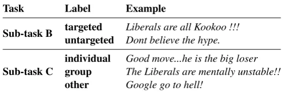
• Sub-task Bis automatic categorization of of-fensive content types, which involves cate-gorizing tweets intotargeted anduntargeted threats. The dataset for this sub-task consists of 4,400 tweets (3,876targetedand 524 un-targeted). Table 1provides one examples of each of these two classes.

• Sub-task C is offense target identification and includes the 3 classes of targets. These classes are in the set{individual, group, oth-ers}. The dataset for this sub-task consists of

3,876 tweets (2,407individual, 1,074group, and 395other). We similarly provide one ex-ample for each of these classes in Table 1.

We use 80% of the tweets as our training set and the remaining 20% as our validation set for both sub-tasks B and C. We also report our best models on the competition test set, as returned to us by organizers. Table2provides statistics of our data for sub-tasks B and C.

3 Methods

3.1 Pre-Processing

We utilize a simple data pre-processing pipeline involving lower-casing all text, filtering out URLs, usernames, punctuation, irrelevant characters and emojis, and splitting text into word-level tokens.

3.2 Data Intelligence Methods

We employ multiple machine learning methods and combine them with different sampling and data generation techniques to enhance our training set. From a data sampling perspective, the most common approaches to deal with imbalanced data is random oversampling and random undersam-pling (Lohr,2009;Chawla,2009). Learning with these basic techniques is usually effective due to possibly reducing model bias towards the major-ity class. We employ a number of data sampling techniques, as described next.

Random oversampling technique randomly duplicates the minority samples to obtain a bal-anced dataset. Despite the naive approach, this method is reported to perform well (as compared to other sophisticated oversampling methods) in the literature. One major drawback of this method is that it does not add any new data to the training set (since it only duplicates minority-class training data) (Liu et al.,2007).

Synthetic minority over-sampling (SMOTE)

is a sophisticated oversampling technique where synthetic samples are generated and added to the minority class. For each data point, one ofk mi-nority class neighbours is randomly selected and the new synthetic point is a random point on the line joining the actual data point and this randomly selected neighbour. This method has been shown to be effective compared to some other oversam-pling methods (Chawla et al.,2002;Batista et al.,

2004).

ob-Task Label Example

Sub-task B targeted Liberals are all Kookoo !!! untargeted Dont believe the hype.

Sub-task C

individual Good move...he is the big loser

group The Liberals are mentally unstable!!

other Google go to hell!

Table 1: Examples of each class in sub-tasks B and C

Task Label Train Dev Total

Sub-task B targeted 3,101 775 3,876 untargeted 419 105 524

Sub-task C

individual 1,925 482 2,407

group 859 215 1,074

other 316 79 395

Table 2: Distribution of classes over our data splits

tain a balanced dataset. One possible disadvantage of this method is that it might remove valuable in-formation from training data since, due to its ran-domness, it does not pay consideration to the data points removed (Liu et al.,2007).

kNN-based undersampling is an alternative undersampling technique (Mani and Zhang,2003) which uses distance between points within a class. We use three different methods to select near-miss samples, as described in Mani and Zhang(2003).

NearMiss-1selects majority class samples whose average distance to three closest minority class samples is smallest. InNearMiss-2, the samples of the majority class are selected such that their av-erage distances to three farthest samples of minor-ity class are smallest. NearMiss-3picks a given number of the closest majority class samples from each minority class sample, which guarantees ev-ery minority class sample is surrounded by some majority class points. Mani and Zhang (2003) choose the majority class samples whose average distances to the three closest minority class sam-ples are farthest.

Synthetic Data Generation. We experiment with adding information to the minority class by generating synthetic samples employing a word2vec-aided paraphrasing technique. Initially, we train a word2vec model on the entire training data and use this word2vec model to generate sam-ples for the minority class by randomly replacing words in tweets (with a probability of 0.9). We

randomly pick one word from k word2vec most similar words. We fix k=5 words and probabil-ity value as 0.9, but these are hyperparameters that can be optimized. In this way, we generate a bal-anced dataset in an attempt to overcome the prob-lem of imbalance. In this technique, we draw in-spiration from (Li et al.,2018) where authors pro-pose a sentiment lexicon generation method us-ing a label propagation algorithm and utilize the generated lexicons to obtain synthetic samples for the minority class by randomly replacing a set of words with words that have similar semantic con-tent.

3.3 Classifiers

We apply a number of machine learning classi-fiers that are proven to work well for text cate-gorization. Namely, we use logistic regression, support vector machines (SVM) and Naive Bayes. We also experiment with boosting algorithms such as random forest, AdaBoost, bagging classifier, XGBoost, and gradient boosting classifier. We de-ploy ensembles of our best performing models in two ways: (1) ensembles based on majority rule classifiers that use predicted class labels for ma-jority rule voting and (2) soft voting classifiers that predict the class label based on the argmax of the sums of the predicted probabilities of various clas-sifiers.

4 Sub-Task B Models

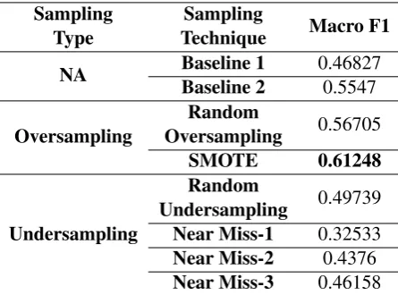
extract features from the tweets and run with un-igrams and all different combinations of unigram, bigrams, trigrams, and four grams. We run on all combinations across all the three variables above (n-grams, classifiers, and sampling methods) on both the imbalanced (ORG) and balanced datasets. Since our datasets are small, this iteration of ex-periments is not very costly. We acquire best re-sults on the balanced dataset, identifying the com-bination of unigrams and bigrams as our best n-gram settings, XGBoost as the best classifier, and SMOTE as the best sampling technique. We pro-vide these best results in Table 3 in Macro-F1 score. We use two baselines. Baseline 1 is the majority class in training data (i.e., targeted of-fense class, 0.46827 Macro F1-score). The sec-ond baseline is the best model with no data sam-pling, a logistic regression model. The best model, XGBoost with SMOTE sampling, acquires an F1 -score of 0.61248. This is a sizeable gain over the baselines. We now describe how we leverage en-sembles to improve over this XGBoost model.

Sampling Type

Sampling

Technique Macro F1

NA Baseline 1 0.46827

Baseline 2 0.5547

Oversampling

Random

Oversampling 0.56705

SMOTE 0.61248

Undersampling

Random

Undersampling 0.49739 Near Miss-1 0.32533

Near Miss-2 0.4376

Near Miss-3 0.46158

Table 3: Sub-Task B: XGBoost performance with sampling methods. Baseline 1 is our majority class in training data. Baseline 2 is a logistic regression model with no data sampling.

4.1 Ensembles for Sub-Task B

Our best performance with the XGBoost model in the previous section was acquired with SMOTE oversampling. However, we note that overpling in general performed better than other sam-pling methods. For this reason, we experiment with a number of ensemble methods across our two oversampling techniques (SMOTE and ran-dom oversampling [ROS]). We provide our best results from this iteration of experiments (for both the dev and the competition test set) in Table 4. In

addition to the same XGBoost model reported ear-lier (in Table 3, reproduced in Table 4), we iden-tify and report our two best models: (1)Model A: An ensemble with soft voting over XGBoost, Ad-aBoost, and logistic regression with random over-sampling (ROS) and (2) Model B: The average of our XGBoost model (with SMOTE) and the best model with synthetic oversampling (which is a Naive Bayes classifier). We submitted the three models in Table 4 to the competition. Although Model B performs best on the dev set, it was model A that performed highest on the competi-tion test set. This suggests that the dev and test sets are different in some aspects. Importantly, even though the three models in Table 4perform com-parably on dev, only the ensemble models (Model A and Model B) seem to generalize better on the test set. This further demonstrates the utility of ensembles on the task.

5 Sub-Task C Models

Sub-Task C is 3-way classification, with 2 minor-ity classes. Again, we run all our classifiers with unigram and bigram combinations across all sam-pling methods (including no samsam-pling) on this im-balanced dataset. In addition, we use 4 differ-ent configurations to generate samples for each of the two minority classes to obtain 4 balanced datasets. C1 is created with random oversam-pling of the two minority classes; C2 is created with synthetic oversampling of the two minority classes; C3is created with random oversampling of minority classgroup(GRP) and synthetic over-sampling of minority classother(OTH); andC4is random oversampling of minority class OTH and synthetic oversampling of minority class GRP.

We report our best results in Table 5, with two baselines: Baseline 1 is the majority class in train-ing data and Baseline 2 is our best model with-out sampling (a logistic regression classifier). Our best model on C2 is a logistic regression classi-fier, whereas our best models on C1, C3, and C4 are acquired with the same soft voting ensemble in Table 4 (an ensemble of logistic regression, Ad-aBoost, and XGBoost).

Our next step is to investigate whether we can further improve performance by averaging classi-fication probabilities of models described in Table

Dataset Models Targeted Untargeted

Precision Recall F1 Precision Recall F1 Macro F1 score

DEV

XGBoost (SMOTE) 0.90158 0.95742 0.92866 0.42105 0.22857 0.2963 0.61248 Model A 0.90945 0.89419 0.90176 0.30508 0.34286 0.32287 0.61231 Model B 0.94065 0.90447 0.9222 0.26667 0.37838 0.31285 0.61753

TEST

XGBoost (SMOTE) 0.9004 0.9765 0.9369 0.4444 0.1481 0.2222 0.57958 Model A 0.9378 0.9202 0.9289 0.4516 0.5185 0.4828 0.70583 Model B 0.9079 0.9718 0.9388 0.5000 0.2222 0.3077 0.62323

Table 4: Sub-Task B:Best ensemble model results. We reproduce XGBoost results from Table 3for comparison.

Sampling Type Best Model Macro F1

NA NA Baseline-1 0.21300

NA Baseline-2 0.51580

Sampling

C1 Model 1 0.56822

C2 Log Reg 0.54319

C3 Model 1 0.54665

C4 Model 1 0.56216

Table 5: Sub-Task C:Best results with various sam-pling methods.

follows:Model 1: our best model with C1;Model 2: a prediction based on the average of classifica-tion probabilities of the best classifiers on C1, C2, and C4;Model 3: the prediction acquired from the average of tag probabilities of the best classifiers on C1 and C4. Table6shows that performance of all the models on the dev set is very comparable, with model 3 performing slightly better than the two other models. Similarly, results of the three models are not very different on the competition test set.

6 Model Analysis

In order to further understand the results on the test set, we investigate the predictions made by our models across the two sub-tasks. For the purpose, we provide simple visualizations of the confusion matrices of predictions acquired by our best mod-els as released by organizers.

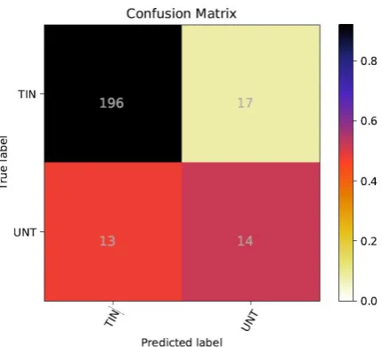
Sub-Task B.Figure 1shows that our model has higher precision for the targeted threats, which is also clear from Table 4presented earlier. Figure

1 also shows that our model has slightly higher false negatives as compared to false positives. In other words, the chances of our model mislabeling a targeted tweet as untargeted is slightly higher as compared to predicting anuntargetedtweet as targeted.

Sub-Task CWe visualize model errors in Fig-ure 2. Figure 2 shows that our model has

Figure 1: Confusion matrix of soft voting ensemble model (Model A in Table 4) for Sub-Task B.

Dataset Models GRP IND OTH Macro F1 score

DEV

Model 1 0.60538 0.82476 0.27451 0.56822

Model 2 0.61504 0.8204 0.28931 0.57492

Model 3 0.61207 0.8203 0.29577 0.57605

TEST

Model 1 0.7101 0.8116 0.2400 0.58722

Model 2 0.686 0.8098 0.2041 0.56663

Model 3 0.6946 0.819 0.2449 0.58619

Table 6: Sub-Task C:Results of our 3 final submitted models

higher precision for thegroup(GRP) and individ-ual (IND) categories, but only higher recall for theother(OTH) class. Again, this means that the chances of our model predicting a GRP tweet or IND tweet as OTH is much higher as compared to OTH tweet being predicted as IND or GRP. In other words, the model is biased towards predict-ing one of the two categories GRP and IND

7 Conclusion

In this paper, we described our contributions to Of-fenseEval, the 6th shared task of SemEval-2019 . We explored the effectiveness of different sam-pling techniques and ensembling methods com-bined with different classical and boosting ma-chine learning algorithms. We find simple data en-hancement approaches (i.e., sampling techniques) to work well, especially when coupled with the right ensemble methods. In general, ensemble models decrease errors by leveraging the differ-ent strengths of the various underlying models and hence are useful in absence of balanced data.

8 Acknowledgement

We acknowledge the support of the Natural Sciences and Engineering Research Council of Canada (NSERC) and the Social Sciences Re-search Council of Canada (SSHRC). The re-search was partially enabled by WestGrid (www. westgrid.ca) and Compute Canada (www. computecanada.ca).

References

Ali Alshehri, AlMoetazbillah Nagoudi, Alhuzali Has-san, and Muhammad Abdul-Mageed. 2018. Think before your click: Data and models for adult content in arabic twitter. The 2nd Text Analytics for Cyber-security and Online Safety (TA-COS-2018), LREC.

Gustavo E. A. P. A. Batista, Ronaldo C. Prati, and Maria Carolina Monard. 2004. A study of the be-havior of several methods for balancing machine

learning training data. SIGKDD Explor. Newsl., 6(1):20–29.

Nitesh V Chawla. 2009. Data mining for imbalanced datasets: An overview. InData mining and knowl-edge discovery handbook, pages 875–886. Springer.

Nitesh V Chawla, Kevin W Bowyer, Lawrence O Hall, and W Philip Kegelmeyer. 2002. Smote: synthetic minority over-sampling technique. Journal of artifi-cial intelligence research, 16:321–357.

Nadia FF Da Silva, Eduardo R Hruschka, and Este-vam R Hruschka Jr. 2014. Tweet sentiment analy-sis with classifier ensembles.Decision Support Sys-tems, 66:170–179.

Thomas Davidson, Dana Warmsley, Michael Macy, and Ingmar Weber. 2017. Automated hate speech detection and the problem of offensive language. InEleventh International AAAI Conference on Web and Social Media.

Vinodhini Gopalakrishnan and Chandrasekaran Ra-maswamy. 2014. Sentiment learning from imbal-anced dataset: an ensemble based method. Int. J. Artif. Intell, 12(2):75–87.

Yijing Li, Haixiang Guo, Qingpeng Zhang, Mingyun Gu, and Jianying Yang. 2018. Imbalanced text sen-timent classification using universal and domain-specific knowledge. Knowledge-Based Systems, 160:1–15.

Alexander Liu, Joydeep Ghosh, and Cheryl E Martin. 2007. Generative oversampling for mining imbal-anced datasets. InDMIN, pages 66–72.

Sharon L Lohr. 2009. Sampling: design and analysis. Nelson Education.

Inderjeet Mani and I Zhang. 2003. knn approach to un-balanced data distributions: a case study involving information extraction. InProceedings of workshop on learning from imbalanced datasets, volume 126.

Asmaa Mountassir, Houda Benbrahim, and Ilham Berrada. 2012. Addressing the problem of unbal-anced data sets in sentiment analysis. In KDIR, pages 306–311.

Nazlia Omar, Mohammed Albared, Adel Qasem Al-Shabi, and Tareq Al-Moslmi. 2013. Ensemble of classification algorithms for subjectivity and senti-ment analysis of arabic customers’ reviews. Interna-tional Journal of Advancements in Computing Tech-nology, 5(14):77.

Aytu˘g Onan, Serdar Koruko˘glu, and Hasan Bulut. 2016. Ensemble of keyword extraction methods and classifiers in text classification. Expert Systems with Applications, 57:232–247.

Georgios K Pitsilis, Heri Ramampiaro, and Helge Langseth. 2018. Detecting offensive language in tweets using deep learning. arXiv preprint arXiv:1801.04433.

Shuo Wang and Xin Yao. 2009. Diversity analysis on imbalanced data sets by using ensemble models. In2009 IEEE Symposium on Computational Intelli-gence and Data Mining, pages 324–331. IEEE.

Rui Xia, Chengqing Zong, and Shoushan Li. 2011. En-semble of feature sets and classification algorithms for sentiment classification. Information Sciences, 181(6):1138–1152.

Guang Xiang, Bin Fan, Ling Wang, Jason Hong, and Carolyn Rose. 2012. Detecting offensive tweets via topical feature discovery over a large scale twit-ter corpus. In Proceedings of the 21st ACM inter-national conference on Information and knowledge management, pages 1980–1984. ACM.

Marcos Zampieri, Shervin Malmasi, Preslav Nakov, Sara Rosenthal, Noura Farra, and Ritesh Kumar. 2019a. Predicting the Type and Target of Offensive Posts in Social Media. InProceedings of NAACL.