Probabilistic Context Free Grammar Induction Based on Structural Zeros

Proceedings of the Human Language Technology Conference of the North American Chapter of the ACL, pages 312–319,

Probabilistic Context-Free Grammar Induction

Based on Structural Zeros

Courant Institute of Mathematical Sciences and Google Research

251 Mercer Street New York, NY 10012 [email protected]

Brian Roark

Center for Spoken Language Understanding OGI at Oregon Health & Science University

20000 NW Walker Road Beaverton, Oregon 97006 [email protected]

Abstract

We present a method for induction of con-cise and accurate probabilistic context-free grammars for efficient use in early stages of a multi-stage parsing technique. The method is based on the use of statis-tical tests to determine if a non-terminal combination is unobserved due to sparse data or hard syntactic constraints. Ex-perimental results show that, using this method, high accuracies can be achieved with a non-terminal set that is orders of magnitude smaller than in typically induced probabilistic context-free gram-mars, leading to substantial speed-ups in parsing. The approach is further used in combination with an existing reranker to provide competitive WSJ parsing results.

1 Introduction

There is a very severe speed vs. accuracy tradeoff in stochastic context-free parsing, which can be ex-plained by the grammar factor in the running-time complexity of standard parsing algorithms such as the CYK algorithm (Kasami, 1965; Younger, 1967). That algorithm has complexityO(n3|P|), wherenis the length in words of the sentence parsed, and|P|is the number of grammar productions. Grammar non-terminals can be split to encode richer dependen-cies in a stochastic model and improve parsing ac-curacy. For example, the parent of the left-hand side (LHS) can be annotated onto the label of the LHS category (Johnson, 1998), hence differentiating, for instance, between expansions of a VP with parent S and parent VP. Such annotations, however, tend to substantially increase the number of grammar pro-ductions as well as the ambiguity of the grammar, thereby significantly slowing down the parsing

algo-rithm. In the case of bilexical grammars, where cat-egories in binary grammars are annotated with their lexical heads, the grammar factor contributes an ad-ditionalO(n2|VD|3)complexity, leading to an

over-all O(n5_|V

D|3) parsing complexity, where |VD| is

the number of delexicalized non-terminals (Eisner, 1997). Even with special modifications to the ba-sic CYK algorithm, such as those presented by Eis-ner and Satta (1999), improvements to the stochastic model are obtained at the expense of efficiency.

In addition to the significant cost in efficiency, increasing the non-terminal set impacts parame-ter estimation for the stochastic model. With more productions, much fewer observations per production are available and one is left with the hope that a subsequent smoothing technique can effectively deal with this problem, regardless of the number of non-terminals created. Klein and Manning (2003b) showed that, by making certain linguistically-motivated node label annotations, but avoiding certain other kinds of state splits (mainly lexical annotations) models of relatively high accu-racy can be built without resorting to smoothing. The resulting grammars were small enough to al-low for exhaustive CYK parsing; even so, parsing speed was significantly impacted by the state splits: the test-set parsing time reported was about 3s for average length sentences, with a memory usage of 1GB.

This paper presents an automatic method for de-ciding which state to split in order to create concise and accurate unsmoothed probabilistic context-free grammars (PCFGs) for efficient use in early stages of a multi-stage parsing technique. The method is based on the use of statistical tests to determine if a non-terminal combination is unobserved due to the limited size of the sample (sampling zero) or because it is grammatically impossible (structural

zero). This helps introduce a relatively small number

of new non-terminals with little additional parsing

NP

@ @PP

P P

DT JJ NN NNS

NP

H H H

DT NP:JJ+NN+NNS

HHH JJ NP:NN+NNS

HH

NN NNS

NP

HHH

DT NP:JJ+NN

HHH JJ NP:NN+NNS

HH

NN NNS

NP

HH

DT NP:JJ

HH

JJ NP:NN

HH

NN NNS

NP

HH

DT NP:

HH

JJ NP:

HH

NN NNS

(a) (b) (c) (d) (e)

Figure 1: Five representations of ann-ary production,n = 4. (a) Original production (b) factored production (c) Right-factored Markov order-2 (d) Right-Right-factored Markov order-1 (e) Right-Right-factored Markov order-0

overhead. Experimental results show that, using this method, high accuracies can be achieved with orders of magnitude fewer non-terminals than in typically induced PCFGs, leading to substantial speed-ups in parsing. The approach can further be used in combi-nation with an existing reranker to provide competi-tive WSJ parsing results.

The remainder of the paper is structured as fol-lows. Section 2 gives a brief description of PCFG induction from treebanks, including non-terminal label-splitting, factorization, and relative frequency estimation. Section 3 discusses the statistical criteria that we explored to determine structural zeros and thus select non-terminals for the factored PCFG. Fi-nally, Section 4 reports the results of parsing experi-ments using our exhaustivek-best CYK parser with the concise PCFGs induced from the Penn WSJ tree-bank (Marcus et al., 1993).

2 Grammar induction

A context-free grammarG= (V, T, S†, P), or CFG in short, consists of a set of non-terminal symbolsV, a set of terminal symbolsT, a start symbolS†∈V, and a set of production P of the form: A → α, where A ∈ V and α ∈ (V ∪T)∗. A PCFG is a CFG with a probability assigned to each production. Thus, the probabilities of the productions expanding a given non-terminal sum to one.

2.1 Smoothing and factorization

PCFGs induced from the Penn Treebank have many productions with long sequences of non-terminals on the RHS. Probability estimates of the RHS given the LHS are often smoothed by making a Markov assumption regarding the conditional independence of a category on those more thankcategories away

(Collins, 1997; Charniak, 2000):

P(X →Y1...Yn)= P(Y1|X)

n

Y

i=2

P(Yi|X, Y1· · ·Yi−1)

≈P(Y1|X)

n

Y

i=2

P(Yi|X, Yi−k· · ·Yi−1).

Making such a Markov assumption is closely re-lated to grammar transformations required for cer-tain efficient parsing algorithms. For example, the CYK parsing algorithm takes as input a Chomsky Normal Form PCFG, i.e., a grammar where all pro-ductions are of the formX → Y Z orX → a, whereX, Y, andZ are non-terminals and aa ter-minal symbol.1_{. Binarized PCFGs are induced from}

a treebank whose trees have been factored so that

n-ary productions withn >2become sequences of

n−1binary productions. Full right-factorization in-volves concatenating the finaln−1 categories from the RHS of ann-ary production to form a new com-posite non-terminal. For example, the original pro-duction NP→DT JJ NN NNS shown in Figure 1(a) is factored into three binary rules, as shown in Fig-ure 1(b). Note that a PCFG induced from such right-factored trees is weakly equivalent to a PCFG in-duced from the original treebank, i.e., it describes the same language.

From such a factorization, one can make a Markov assumption for estimating the production probabilities by simply recording only the labels of the firstkchildren dominated by the composite fac-tored label. Figure 1 (c), (d), and (e) show right-factored trees of Markov orders 2, 1 and 0 respec-tively.2 In addition to being used for smoothing

1_{Our implementation of the CYK algorithm has been} ex-tended to allow for unary productions with non-terminals on the RHS in the PCFG.

2

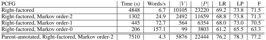
PCFG Time (s) Words/s |V| |P| LR LP F

Right-factored 4848 6.7 10105 23220 69.2 73.8 71.5

Right-factored, Markov order-2 1302 24.9 2492 11659 68.8 73.8 71.3

Right-factored, Markov order-1 445 72.7 564 6354 68.0 73.0 70.5

Right-factored, Markov order-0 206 157.1 99 3803 61.2 65.5 63.3

Parent-annotated, Right-factored, Markov order-2 7510 4.3 5876 22444 76.2 78.3 77.2

Table 1: Baseline results of exhaustive CYK parsing using different probabilistic context-free grammars. Grammars are trained from sections 2-21 of the Penn WSJ Treebank and tested on all sentences of section 24 (no length limit), given weightedk-best POS-tagger output. The second and third columns report the total parsing time in seconds and the number of words parsed per second. The number of non-terminals,|V|,is indicated in the next column. The last three columns show the labeled recall (LR), labeled precision (LP), and F-measure (F).

as mentioned above, these factorizations reduce the size of the non-terminal set, which in turn improves CYK efficiency. The efficiency benefit of making a Markov assumption in factorization can be substan-tial, given the reduction of both non-terminals and productions, which improves the grammar constant. With standard right-factorization, as in Figure 1(b), the non-terminal set for the PCFG induced from sec-tions 2-21 of the Penn WSJ Treebank grows from its original size of 72 to 10105, with 23220 produc-tions. With a Markov factorization of orders 2, 1 and 0 we get non-terminal sets of size 2492, 564, and 99, and rule production sets of 11659, 6354, and 3803, respectively.

These reductions in the size of the non-terminal set from the original factored grammar result in an order of magnitude reduction in complexity of the CYK algorithm. One common strategy in statisti-cal parsing is what can be termed an approximate coarse-to-fine approach: a simple PCFG is used to prune the search space to which richer and more complex models are applied subsequently (Char-niak, 2000; Charniak and Johnson, 2005). Produc-ing a “coarse” chart as efficiently as possible is thus crucial (Charniak et al., 1998; Blaheta and Charniak, 1999), making these factorizations particularly use-ful.

2.2 CYK parser and baselines

To illustrate the importance of this reduction in non-terminals for efficient parsing, we will present base-line parsing results for a development set. For these baseline trials, we trained a PCFG on sec-tions 2-21 of the Penn WSJ Treebank (40k sen-tences, 936k words), and evaluated on section 24 (1346 sentences, 32k words). The parser takes as input the weighted k-best POS-tag sequences of a

final NNS depends on the preceding NN, despite the Markov order-0 factorization. Because of our focus on efficient CYK, we accept these higher order dependencies rather than produc-ing unary productions. Only n-ary rulesn>2are factored.

perceptron-trained tagger, using the tagger docu-mented in Hollingshead et al. (2005). The number of tagger candidates kfor all trials reported in this paper was 0.2n, wherenis the length of the string. From the weighted k-best list, we derive a condi-tional probability of each tag at positioniby taking the sum of the exponential of the weights of all can-didates with that tag at positioni(softmax).

The parser is an exhaustive CYK parser that takes advantage of the fact that, with the grammar fac-torization method described, factored non-terminals can only occur as the second child of a binary pro-duction. Since the bulk of the non-terminals result from factorization, this greatly reduces the number of possible combinations given any two cells. When parsing with a parent-annotated grammar, we use a version of the parser that also takes advantage of the partitioning of the non-terminal set, i.e., the fact that any given non-terminal has already its parent indi-cated in its label, precluding combination with any non-terminal that does not have the same parent an-notated.

(2003b)3.

From these results, we can see the large efficiency benefit of the Markov assumption, as the size of the non-terminal and production sets shrink. However, the efficiency gains come at a cost, with the Markov order-0 factored grammar resulting in a loss of a full 8 percentage points of F-measure accuracy. Parent annotation provides a significant accuracy improve-ment over the other baselines, but at a substantial efficiency cost.

Note that the efficiency impact is not a strict func-tion of either the number of non-terminals or pro-ductions. Rather, it has to do with the number of competing non-terminals in cells of the chart. Some grammars may be very large, but less ambiguous in a way that reduces the number of cell entries, so that only a very small fraction of the productions need to be applied for any pair of cells. Parent annotation does just the opposite – it increases the number of cell entries for the same span, by creating entries for the same constituent with different parents. Some non-terminal annotations, e.g., splitting POS-tags by annotating their lexical items, result in a large gram-mar, but one where the number of productions that will apply for any pair of cells is greatly reduced.

Ideally, one would obtain the efficiency benefit of the small non-terminal set demonstrated with the Markov order-0 results, while encoding key gram-matical constraints whose absence results in an ac-curacy loss. The method we present attempts to achieve this by using a statistical test to determine

structural zeros and modifying the factorization to

remove the probability mass assigned to them.

3 Detecting Structural Zeros

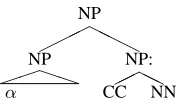
The main idea behind our method for detecting structural zeros is to search for events that are in-dividually very frequent but that do not co-occur. For example, consider the Markov order-0 bi-nary rule production in Figure 2. The produc-tion NP→NP NP: may be very frequent, as is the NP:→CC NN production, but they never co-occur together, because NP does not conjoin with NN in the Penn Treebank. If the counts of two such eventsaandb, e.g., NP→NP NP: and NP:→CC NN are very large, but the count of their co-occurrence

3

Their Markov order-2 factorization does not follow the lin-ear order of the children, but rather includes the head-child plus one other, whereas our factorization does not involve identifica-tion of the head child.

NP

H H H NP

PP

α

NP: HH

CC NN

Figure 2: Markov order-0 local tree, with possible non-local ¡state-split information.

is zero, then the co-occurrence of a and b can be viewed as a candidate for the list of events that are structurally inadmissible. The probability mass for the co-occurrence of a and b can be removed by replacing the factored non-terminal NP: with NP:CC:NN whenever there is a CC and an NN com-bining to form a factored NP non-terminal.

The expansion of the factored non-terminals is not the only event that we might consider. For exam-ple, a frequent left-most child of the first child of the production, or a common left-corner POS or lexi-cal item, might never occur with certain productions. For example, ‘SBAR→IN S’ and ‘IN→of’ are both common productions, but they never co-occur. We focus on left-most children and left-corners because of the factorization that we have selected, but the same idea could be applied to other possible state splits.

Different statistical criteria can be used to com-pare the counts of two events with that of their co-occurrence. This section examines several possible criteria that are presented, for ease of exposition, with general sequences of events. For our specific purpose, these sequences of events would be two rule productions.

3.1 Notation

This section describes several statistical criteria to determine if a sequence of two events should be viewed as a structural zero. These tests can be gen-eralized to longer and more complex sequences, and to various types of events, e.g., word, word class, or rule production sequences.

Given a corpusC, and a vocabularyΣ, we denote by ca the number of occurrences of a inC. Letn

be the total number of observations in C. We will denote by¯athe set {b ∈ Σ : b 6= a}. Hencec¯a =

n−ca. LetP(a) = c_na, and forb∈Σ, letP(a|b) = cab

3.2 Mutual information

The mutual information between two random vari-ablesXandY is defined as

I(X;Y) =X

x,y

P(x, y) log P(x, y)

P(x)P(y). (1)

For a particular event sequence of length twoab, this suggests the following statistic:

I(ab) = log P(ab)−log P(a)−log P(b) = logcab−logca−logcb+ logn

Unfortunately, forcab = 0,I(ab)is not finite. If we

assume, however, that all unobserved sequences are given somecount, then whencab= 0,

I(ab) = K−logca−logcb, (2)

whereKis a constant. Since we need these statistics only for ranking purposes, we can ignore the con-stant factor.

3.3 Log odds ratio

Another statistic that, like mutual information, is ill-defined with zeros, is the log odds ratio:

log(ˆθ) = logcab+ logc¯a¯b−logc¯ab−logca¯b.

Here again, ifcab= 0,log(ˆθ)is not finite. But, if we

assign to all unobserved pairs a small count, when

cab = 0,c¯ab =cb, and the expression becomes

log(ˆθ) =K+ logc_a¯¯_b−logcb−logca. (3)

3.4 Pearson chi-squared

For any i, j ∈ Σ, define µˆij = ci_ncj. The Pearson

chi-squared test of independence is then defined as follows:

X2₌X

i∈ {a,¯a}

j∈˘_b,¯_b¯

(cij−µˆij)2

ˆ

µij = X

i∈ {a,¯a}

j∈˘_b,¯_b¯

(ncij−cicj)2

ncicj .

In the case of interest for us,cab = 0and the statistic

simplifies to:

X2 ₌ cacb

n + c2

acb

nc¯a +

cac2b

nc¯_b +

c2

ac2b

nc¯ac¯_b =

ncacb

c¯ac¯_b . (4)

3.5 Log likelihood ratio

Pearson’s chi-squared statistic assumes a normal or approximately normal distribution, but that assump-tion typically does not hold for the occurrences of rare events (Dunning, 1994). It is then preferable to use the likelihood ratio statistic which allows us to compare the null hypothesis, thatP(b) = P(b|a) = P(b|¯a) = cb

n, with the hypothesis thatP(b|a) = cab

ca

and P(b|¯a) = cab¯

c¯a. In words, the null hypothesis

is that the context of event a does not change the probability of seeingb. These discrete conditional probabilities follow a binomial distribution, hence the likelihood ratio is

λ= B[P(b), cab, ca]B[P(b), c¯ab, c¯a]

B[P(b|a), cab, ca]B[P(b|¯a), c¯ab, ca¯]

, (5)

whereB[p, x, y] = px(1−p)y−x( y

x ).In the

spe-cial case where cab = 0, P(b|¯a) = P(b), and this

expression can be simplified as follows:

λ = (1−P(b))

ca_P(b)cab¯ _(1−P(b))c¯a−cab¯

P(b|¯a)c¯ab₍₁−_P(b|¯_a))c¯a−c¯ab

= (1−P(b))ca_{. (6)}

The log-likelihood ratio, denoted byG2, is known to be asymptoticallyX2_{-distributed. In this case,}

G2 =−2calog(1−P(b)), (7)

and with the binomial distribution, it has has one degree of freedom, thus the distribution will have asymptotically a mean of one and a standard devia-tion of√2.

We experimented with all of these statistics. While they measure different ratios, empirically they seem to produce very similar rankings. For the experiments reported in the next section, we used the log-likelihood ratio because this statistic is well-defined with zeros and is preferable to the Pearson chi-squared when dealing with rare events.

4 Experimental results

We used the log-likelihood ratio statisticG2 to rank unobserved eventsab, wherea⊂P andb∈V. Let

Vo be the original, unfactored non-terminal set, and

letα ∈ (Vo :)∗ be a sequence of zero or more

non-terminal/colon symbol pairs. Suppose we have a fre-quent factored non-terminalX:αB forX, B ∈Vo.

A ∈ Vo is also frequent, but X → Y X:αB is

un-observed, this is a candidate structural zero. Simi-lar splits can be considered with factored non-terminals.

There are two state split scenarios we consider in this paper. Scenario 1 is for factored non-terminals, which are always the second child of a binary pro-duction. For use in Equation 7,

ca =

X

A∈Vo

c(X →Y X:αA)

cb = c(X:αB) forB ∈Vo

cab = c(X→Y X:αB)

P(b) = P c(X:αB)

A∈Voc(X:αA) .

Scenario 2 is for non-factored non-terminals, which we will split using the leftmost child, the left-corner POS-tag, and the left-corner lexical item, which are easily incorporated into our grammar factorization approach. In this scenario, the non-terminal to be split can be either the left or right child in the binary production. Here we show the counts for the left child case for use in Equation 7:

ca =

X

A

c(X→Y[αA]Z)

cb = c(Y[αB])

cab = c(X →Y[αB]Z)

P(b) = Pc(Y[αB])

Ac(Y[αA])

In this case, the possible splits are more compli-cated than just non-terminals as used in factoring. Here, the first possible split is the left child cat-egory, along with an indication of whether it is a unary production. One can further split by in-cluding the left-corner tag, and even further by including the left-corner word. For example, a unary S category might be split as follows: first to S[1:VP] if the single child of the S is a VP; next to S[1:VP:VBD] if the left-corner POS-tag is VBD; finally to S[1:VP:VBD:went] if the VBD verb was ‘went’.

Note that, once non-terminals are split by anno-tating such information, the base non-terminals, e.g., S, implicitly encode contexts other than the ones that were split.

Table 2 shows the unobserved rules with the largest G2 _{score, along with the ten non-terminals}

Unobserved production G2

(added NT(s) in bold) score

PP→IN[that] NP 7153.1

SBAR→IN[that] S[1:VP] 5712.1

SBAR→IN[of] S 5270.5 SBAR→WHNP[1:WDT] S[1:VP:TO] 4299.9

VP→AUX VP[MD] 3972.1

SBAR→IN[in] S 3652.1

NP→NP VP[VB] 3236.2

NP→NN NP:CC:NP 2796.3

SBAR→WHNP S[1:VP:VBG] 2684.9

Table 2: Top ten non-terminals to add, and the unobserved productions leading to their addition to the non-terminal set.

that these productions suggest for inclusion in our non-terminal set. The highest scoring un-observed production is PP → IN[that] NP. It re-ceives such a high score because the base production (PP→IN NP) is very frequent, and so is ‘IN→that’, but they jointly never occur, since ‘IN→that’ is a complementizer. This split non-terminal also shows up in the second-highest ranked zero, an SBAR with ‘that’ complementizer and an S child that consists of a unary VP. The unary S→VP production is very common, but never with a ‘that’ complementizer in an SBAR.

Note that the fourth-ranked production uses two split non-terminals. The fifth ranked rule presum-ably does not add much information to aid parsing disambiguation, since the AUX MD tag sequence is unlikely4. The eighth ranked production is the first with a factored category, ruling out coordination be-tween NN and NP.

Before presenting experimental results, we will mention some practical issues related to the ap-proach described. First, we independently parame-terized the number of factored categories to select and the number of non-factored categories to se-lect. This was done to allow for finer control of the amount of splitting of non-terminals of each type. To choose 100 of each, every non-terminal was as-signed the score of the highest scoring unobserved production within which it occurred. Then the 100 highest scoring non-terminals of each type were added to the base non-terminal list, which originally consisted of the atomic treebank non-terminals and Markov order-0 factored non-terminals.

Once the desired non-terminals are selected, the training corpus is factored, and non-terminals are split if they were among the selected set. Note,

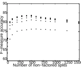
0 250 500 750 1000 1250 1500 60

65 70 75 80 85 90

Number of non−factored splits

F−measure accuracy

Figure 3: F-measure accuracy on development set versus the number of non-factored splits for the given run. Points represent different numbers of factored splits.

ever, that some of the information in a selected non-terminal may not be fully available, requiring some number of additional splits. Any non-terminal that is required by a selected non-terminal will be selected itself. For example, suppose that NP:CC:NP was chosen as a factored non-terminal. Then the sec-ond child of any local tree with that non-terminal on the LHS must either be an NP or a factored non-terminal with at least the first child identified as an NP, i.e., NP:NP. If that factored non-terminal was not selected to be in the set, it must be added. The same situation occurs with left-corner tags and words, which may be arbitrarily far below the cate-gory.

After factoring and selective splitting of non-terminals, the resulting treebank corpus is used to train a PCFG. Recall that we use thek-best output of a POS-tagger to parse. For each POS-tag and lexical item pair from the output of the tagger, we reduce the word to lower case and check to see if the com-bination is in the set of split POS-tags, in which case we split the tag, e.g., IN[that].

Figure 3 shows the F-measure accuracy for our trials on the development set versus the number of non-factored splits parameterized for the trial. From this plot, we can see that 500 non-factored splits provides the best F-measure accuracy on the dev set. Presumably, as more than 500 splits are made, sparse data becomes more problematic. Figure 4 shows the development set F-measure accuracy ver-sus the number of words-per-second it takes to parse the development set, for non-factored splits of 0 and 500, at a range of factored split parameterizations. With 0 non-factored splits, efficiency is substantially impacted by increasing the factored splits, whereas it can be seen that with 500 non-factored splits, that impact is much less, so that the best performance

0 20 40 60 80 100 120 140 160 180 60

65 70 75 80 85 90

Words per second

F−measure accuracy

non−fact. splits=0 non−fact. splits=500 Markov order−0 Markov order−1 Markov order−2 PA, Markov order−2

Figure 4: F-measure accuracy versus words-per-second for (1) no non-factored splits (i.e., only factored categories se-lected); (2) 500 non-factored splits, which was the best perform-ing; and (3) four baseline results.

is reached with both relatively few factored non-terminal splits, and a relatively small efficiency im-pact. The non-factored splits provide substantial ac-curacy improvements at relatively small efficiency cost.

Table 3 shows the 1-best and reranked 50-best re-sults for the baseline Markov order-2 model, and the best-performing model using factored and non-factored non-terminal splits. We present the effi-ciency of the model in terms of words-per-second over the entire dev set, including the longer strings (maximum length 116 words)5. We used thek-best decoding algorithm of Huang and Chiang (2005) with our CYK parser, using on-demandk-best back-pointer calculation. We then trained a MaxEnt reranker on sections 2-21, using the approach out-lined in Charniak and Johnson (2005), via the pub-licly available reranking code from that paper.6 We used the default features that come with that pack-age. The processing time in the table includes the time to parse and rerank. As can be seen from the trials, there is some overhead to these processes, but the time is still dominated by the base parsing.

We present thek-best results to demonstrate the benefits of using a better model, such as the one we have presented, for producing candidates for down-stream processing. Even with severe pruning to only the top 50 candidate parses per string, which re-sults in low oracle and reranked accuracy for the Markov order-2 model, the best-performing model based on structural zeros achieves a relatively high oracle accuracy, and reaches 88.0 and 87.5 percent F-measure accuracy on the dev (f24) and eval (f23) sets respectively. Note that the well-known

Char-5_{The parsing time with our model for average length} sen-tences (23-25 words) is 0.16 seconds per sentence.

6

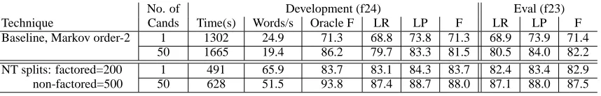
No. of Development (f24) Eval (f23)

Technique Cands Time(s) Words/s Oracle F LR LP F LR LP F

Baseline, Markov order-2 1 1302 24.9 71.3 68.8 73.8 71.3 68.9 73.9 71.4

50 1665 19.4 86.2 79.7 83.3 81.5 80.5 84.0 82.2

NT splits: factored=200 1 491 65.9 83.7 83.1 84.3 83.7 82.4 83.4 82.9

non-factored=500 50 628 51.5 93.8 87.4 88.7 88.0 87.1 88.0 87.5

Table 3: Parsing results on the development set (f24) and the evaluation set (f23) for the baseline Markov order-2 model and the best-performing structural zero model, with 200 factored and 500 non-factored non-terminal splits. 1-best results, plus reranking using a trained version of an existing reranker with 50 candidates.

niak parser (Charniak, 2000; Charniak and Johnson, 2005) uses a Markov order-3 baseline PCFG in the initial pass, with a best-first algorithm that is run past the first parse to populate the chart for use by the richer model. While we have demonstrated ex-haustive parsing efficiency, our model could be used with any of the efficient search best-first approaches documented in the literature, from those used in the Charniak parser (Charniak et al., 1998; Blaheta and Charniak, 1999) to A∗ parsing (Klein and Manning, 2003a). By using a richer grammar of the sort we present, far fewer edges would be required in the chart to include sufficient quality candidates for the richer model, leading to further downstream savings of processing time.

5 Conclusion

We described a method for creating concise PCFGs by detecting structural zeros. The resulting un-smoothed PCFGs have far higher accuracy than sim-ple induced PCFGs and yet are very efficient to use. While we focused on a small number of simple non-terminal splits that fit the factorization we had se-lected, the technique presented is applicable to a wider range of possible non-terminal annotations, including head or parent annotations. More gener-ally, the ideas and method for determining structural zeros (vs. sampling zeros) can be used in other con-texts for a variety of other learning tasks.

Acknowledgments

This material is based upon work supported by the National Science Foundation under Grant IIS-0447214. Any opinions, findings, and conclusions or recommendations expressed in this material are those of the authors and do not necessarily reflect the views of the NSF. The first author’s work was partially funded by the New York State Office of Science Technology and Academic Research (NYS-TAR).

References

D. Blaheta and E. Charniak. 1999. Automatic compensation for parser figure-of-merit flaws. In Proceedings of ACL, pages 513–518.

E. Charniak and M. Johnson. 2005. Coarse-to-fine n-best pars-ing and MaxEnt discriminative rerankpars-ing. In Proceedpars-ings of

ACL, pages 173–188.

E. Charniak, S. Goldwater, and M. Johnson. 1998. Edge-based best-first chart parsing. In Proceedings of the 6th Workshop

on Very Large Corpora, pages 127–133.

E. Charniak. 2000. A maximum-entropy-inspired parser. In

Proceedings of NAACL, pages 132–139.

M.J. Collins. 1997. Three generative, lexicalised models for statistical parsing. In Proceedings of ACL, pages 16–23. T. Dunning. 1994. Accurate Methods for the Statistics

of Surprise and Coincidence. Computational Linguistics,

19(1):61–74.

J. Eisner and G. Satta. 1999. Efficient parsing for bilexical context-free grammars and head automaton grammars. In

Proceedings of ACL, pages 457–464.

J. Eisner. 1997. Bilexical grammars and a cubic-time proba-bilistic parser. In Proceedings of the International Workshop

on Parsing Technologies, pages 54–65.

K. Hollingshead, S. Fisher, and B. Roark. 2005. Comparing and combining finite-state and context-free parsers. In

Pro-ceedings of HLT-EMNLP, pages 787–794.

L. Huang and D. Chiang. 2005. Better k-best parsing. In

Pro-ceedings of the 9th International Workshop on Parsing Tech-nologies (IWPT), pages 53–64.

M. Johnson. 1998. PCFG models of linguistic tree representa-tions. Computational Linguistics, 24(4):617–636.

T. Kasami. 1965. An efficient recognition and syntax analy-sis algorithm for context-free languages. Technical Report, AFCRL-65-758, Air Force Cambridge Research Lab., Bed-ford, MA.

D. Klein and C. Manning. 2003a. A* parsing: Fast exact Viterbi parse selection. In Proceedings of HLT-NAACL. D. Klein and C. Manning. 2003b. Accurate unlexicalized

pars-ing. In Proceedings of ACL.

M.P. Marcus, B. Santorini, and M.A. Marcinkiewicz. 1993. Building a large annotated corpus of English: The Penn Treebank. Computational Linguistics, 19(2):313–330. D.H. Younger. 1967. Recognition and parsing of context-free