A financial accelerator through coordination failure

A Financial Accelerator through

Coordination Failure

A Financial Accelerator through

Coordination Failure

∗

Oliver de Groot

University of St Andrews & European Central Bank

31 January 2019

Abstract

This paper studies the effect of liquidity crises in short-term debt markets in a

dy-namic general equilibrium framework. Creditors (retail banks) receive imperfect signals

regarding the profitability of borrowers (wholesale banks) and, based on these signals

and their beliefs about other creditors actions, choose whether to rollover funding, or

not. The uncoordinated actions of creditors cause a suboptimal incidence of rollover,

generating an illiquidity premium. Leverage magnifies the coordination inefficiency.

Illiquidity shocks in credit markets result in sharp contractions in output. Policy

re-sponses are analyzed.

Keywords: Financial frictions, DSGE models, Global games, Bank runs,

Unconven-tional monetary policy, Financial crises.

JEL Classification: D82, E32, E44, G12

∗_{I would like to thank Chryssi Giannitsarou for her help and support throughout the writing of this paper.}

I am also grateful for helpful comments and discussions from Dean Corbae, Giancarlo Corsetti, Emily de Groot, Wouter den Haan, Stephen Morris, Matthias Paustian, Hashem Pesaran, Sergejs Saksonovs, Flavio Toxvaerd, TengTeng Xu, and the participants at many conferences, central banks and universities. First version: August 2010. Disclaimer: The views expressed in this paper are those of the author and do not necessarily reflect the views of the ECB, the Eurosystem, or its staff.

1

Introduction

Creditors financing a project face a coordination problem. Fear of other creditors not rolling

over funding may lead to preemptive action, undermining the project, and the chance of

repayment to those creditors as well. Coordination problems impact the functioning of many

types of the credit market but often the most visible manifestation of coordination failure

is a bank run.1 _{At least since Bagehot (1873)’s description of the 1866 financial panic,}

economists have acknowledged the inherent fragility of financial intermediaries. Table 1 lists

notable bank runs during the 2007-08 financial crisis. The demise of Northern Rock (UK)

and Lehman Brothers (US), for example, have been interpreted (see Brunnermeier (2009)

and Shin (2009)) as events in which short-term interbank market creditors were unwilling to continue lending to these institutions, for fear that other creditors were doing likewise.2

This paper makes three contributions. First, it builds a rigorously micro-founded

coor-dination problem in credit markets in a dynamic, general equilibrium macroeconomic model.

Second, the model highlights the role that maturity- and liquidity-mismatch play in the

prop-agation of shocks through the economy. Third, it provides a laboratory to study the effect of

unconventional policy responses to a large scale liquidity dry up, as seen during the 2007-08

financial crisis.

To the best of my knowledge, this paper was the first to model liquidity and bank runs

within a dynamic general equilibrium framework.3 Recently, Gertler and Kiyotaki (2015) and Gertler et al. (2016) also studied the macroeconomic implications of bank runs. My

contribution distinguishes itself from these in two important respects. First, in the

afore-mentioned papers bank runs are themselves aggregate shocks to the economy in which the

entire financial sector experiences a run. In reality, as Table 1 suggests, even during a major

financial crisis, only a subset of all financial institutions experience a run. My model

cap-tures this feature. In particular, in any given period the proportion of borrowers in danger

1_{Coordination problems also impact the market for bank loans, commercial paper, and corporate bonds.}

For example, Hertzberg et al. (2011) exploited a natural experiment, which compelled banks to make public negative private assessments about their borrowers, to quantify the effect of coordination problems. Even the commercial paper market, primarily for low-default-risk firms, experienced liquidity dry ups, following the Penn Central bankruptcy (1970), the Russia/LTCM crisis (1998), and the Enron/WorldCom episode (2002). In 2008, the Fed introduced the Commercial Paper Funding Facility (CPFF) to prevent a market freeze. No issuers who used the CPFF defaulted on their debt obligations, suggesting the liquidity dry up was driven by coordination problems rather than increased insolvency risk. Disorderly liquidation of assets is economically inefficient. In the US, chapter 11 bankruptcy provision is designed to address the coordination problem among creditors (Jackson (1986)), giving legal protection to a firm to remain in business while being restructured.

2_{In practice, it is difficult to disentangle whether the unwillingness of creditors to continue lending hastened}

the bankruptcy of an insolvent bank or whether the run scuppered a sound institution. Morris and Shin (2016) disentangle the two in theory.

of experiencing a run is determined by the aggregate state, with the proportion of borrowers

experiencing a run being endogenously countercyclical. Second, runs in the model are

deter-mined by a rigorously microfounded global game. In contrast, Gertler and Kiyotaki (2015) and Gertler et al. (2016) use an ad hoc threshold rule (based on the insights from the global

games literature).

Table 1: Notable bank runs during the 2007-08 financial crisis

2007 Aug Countrywide Financial US Wholesale funding run followed by a retail-deposit run.

2007 Sep Northern Rock UK Wholesale funding run followed by a retail-deposit run.

2008 Mar Bear Stearns US Wholesale funding run.

2008 Jul IndyMac US Wholesale funding and brokered-deposit run.

2008 Sep Lehman Brothers US Wholesale funding run.

2008 Sep Washington Mutual US Retail deposit run.

2008 Sep Wachovia US Retail- and brokered-deposit bank run.

In my model, wholesale banks (the borrowers) finance themselves with short-term debt from a multitude of retail banks (the creditors). I show that coordination problems generate an equilibrium trade off between the leverage of a borrower and the illiquidity premium paid

on external finance, resulting from a suboptimal incidence of debt rollover. The coordination

problems among creditors amplify business cycle dynamics and illiquidity shocks in credit

markets generate a novel channel for additional volatility in economic activity. I study two

potential policy instruments to dampen the effect of an illiquidity crisis: direct lending to and equity injections into wholesale banks. I show, for a given dollar amount committed, that equity injections dampen the contemporaneous effect on economic activity more than direct

lending, but causes output to remain subdued for longer. This is because a dollar of debt

intermediated by the policymaker improves the solvency of a wholesale bank (which largely

determines the extent of the coordination problem) by less than a dollar of additional

eq-uity. However, equity injections disincentivize balance sheet adjustment, slowing the output

recovery following the shock.

Coordination failure arises from two assumptions. One, borrowers have a balance sheet

maturity mismatch with longer maturity (more illiquid) assets and shorter maturity (more

liquid) liabilities. Two, multiple creditors per borrower who cannot coordinate their actions. When a borrower’s debt matures, each creditor must decide whether to rollover, taking

ac-count of fundamentals and the actions of other creditors. Diamond and Dybvig (1983) study

equilibria, one of which is a bank run.4 Such multiple equilibria, however, are problematic for

a general equilibrium framework where the endogenous pricing of a debt contract requires

ex ante knowledge about the probability distribution of ex post outcomes. Global games offer a solution.5 _{Multiple equilibria in Diamond and Dybvig (1983) is a consequence of the}

assumption that creditors’ information sets are perfectly symmetric. By introducing

idiosyn-cratic noise into creditors’ signal of a borrower’s solvency, the global games literature shows

that a unique set of self-fulfilling beliefs prevail in equilibrium. I thus model the coordination

problem in credit markets as a sequence of micro-founded static global games, building on

Morris and Shin (2004), Rochet and Vives (2004), and Goldstein and Pauzner (2005). The

resulting dynamic general equilibrium model allows the study of the macroeconomic effects

of illiquidity shocks and the efficacy of alternative policy interventions.6

Liquidity hoarding and interbank lending during the crisis has been studied Heider et al. (2015). However, theories of coordination problems in credit markets have received

rela-tively little attention in the macroeconomics literature. The majority of the financial friction

literature has broadly followed two paths which find their roots in the work of Bernanke and

Gertler (1989) (building on the costly state verification (CSV) assumption from Townsend

(1979), in which there is an informational asymmetry in a single borrower-creditor

relation-ship) and Kiyotaki and Moore (1997) (building on the hold-up assumption of Hart and Moore

(1994), introducing a binding collateral constraint on lending).7 The distortion created by

coordination problems among creditors is a distinct and important feature of credit

mar-kets, especially during the 2007-08 financial crisis. This paper therefore is an important complementary framework to analyze credit market interventions. Related papers modeling

the policy response of the Fed, Treasury, and other central banks and governments to the

financial crisis in the context of alternative financial frictions include Gertler and Kiyotaki

(2010) and Gertler and Karadi (2011).8

The rest of the paper: Section 2 presents the model. Section 3 analyzes partial

equi-librium comparative statics of the global game and the dynamic response of the model to

illiquidity shocks. Section 4 analyzes direct lending and equity injections. Section 5

con-cludes.

4_{See Gorton and Winton (2003) for a review of the literature Diamond and Dybvig (1983) spawned.}

5_{The seminal contribution is Carlsson and van Damme (1993). For an overview, see Morris and Shin}

(2003). Corsetti et al. (2004) apply global games to currency crises.

6_{Kurlat (2013) and Dang et al. (2012) explain why the market for some assets freeze during crises.}

7_{Seminal contributions include Carlstrom and Fuerst (1997) and Bernanke et al. (1999); Iacoviello (2005)}

applied financial frictions to the housing market; Christiano et al. (2014) estimated the importance of financial risk shocks; Carlstrom et al. (2010), Fiore and Tristani (2013), and C´urdia and Woodford (2016) analyze optimal monetary policy with financial frictions; Angeloni and Faia (2013) model macroprudential policy. de Groot (2016) reviews the financial accelerator literature.

2

The model

The model is a canonical real business cycle model in which I embed a coordination problem

facing retail banks in financing wholesale banks.

2.1

Households

A representative household consumes, Ct, supplies labor, Lt, and has preferences given by

E0 ∞

X

t=0

βt

C1−σC

t

1−σC

−χL

1+ρ t

1 +ρ

. (1)

The household maximizes (1) subject to its budget constraint given by

Ct ≤WtLt+Rt−1Dt−1−Dt+ Πt, (2)

where Wt is the real wage, Rt is a predetermined risk-free rate on deposits held with retail

banks, Πt are profits (from owning goods producing firms and capital producers). The

household’s first-order conditions are given by

Wt=χL ρ tC

σC

t , (3)

1 =β_Et(Ct+1/Ct) −σC_R

t. (4)

2.2

Capital producers

The production of new capital is subject to adjustment costs. A representative capital

producer takes It consumption goods and transforms them into Ψ (It/I)I units of capital

that it sells at priceQt(whereI is the steady state level of investment). I assume the function

Ψ is concave and Ψ(1) = Ψ0(1) = 1 and Ψ00(1) =−ψ. Profits are given by QtΨ (It/I)I−It.

The producer’s first-order condition is given by

Qt = (Ψ0(It/I)) −1

. (5)

The aggregate capital stock at the end of period t is given by

Kt = (1−δ)Kt∗ + Ψ (It/I)I, (6)

2.3

Goods producers

Goods producing firms hire labor and rent capital as inputs to a constant returns to scale

technology to produce output, Yt, given by

Yt =At(Kt∗) α

L1−_t α, (7)

where At is the stochastic level of technology. Output is sold in a perfectly competitive

market at a unit price. The firm’s first-order conditions are given by

M P Kt=αYt/Kt∗, (8)

Wt= (1−α)Yt/Lt, (9)

where M P Kt is the marginal product of capital. In the absence of coordination failure,

arbitrage ensures that the discounted expected return on capital equals the risk-free rate

Et (Ct+1/Ct) −σC_R

K,t+1

=_Et (Ct+1/Ct)

−σC_R

t, (10)

where RK,t ≡(M P Kt+ (1−δ)Qt)/Qt−1.

2.4

Retail and wholesale banks

The financial sector transforms household savings into financing for firms to rent capital.

Two types of intermediary exist: retail and wholesale banks. Retail banks accept household

savings and lend to wholesale banks who finance firms. By assumption, wholesale banks rely

on short-term debt funding from a large number of retail banks. As a result, retail banks

face a coordination problem in deciding whether to rollover maturing debt.

Wholesale banks Think of them as capital managers. They invest in firms’ capital with the intention of augmenting the capital with their idiosyncratic productivity and earning

a return from the augmented capital. Formally, there is a continuum of wholesale banks

indexed by w with preferences linear in consumption. At the end of t − 1, a wholesale bank purchases capital, Kwt−1, at price Qt−1 financed with net worth, Nwt−1, and external

financing from the full continuum of retail banks. This external finance takes the form of

a two-stage intertemporal loan: 1) At an intra-period stage of time t retail banks decide whether to rollover the loan. 2) Rolled over loans are scheduled for repayment at the end of

a return at the end of t but its liabilities (the debt) must be rolled intra-period.9

At the end oft−1 wholesale banks are homogeneous in all respects except net worth. Thus, wholesale bank leverage, `t = QtKwt/Nwt, and the terms of the debt contract (such

as the loan rate) will be common across banks. At the beginning of t, wholesale bank w

observes its idiosyncratic productivity that will transform its capital to ωwtKwt−1, where ωwt

is iid across time and space, _E(ωwt) = 1, with cdf F, pdf f, and support on [0,∞). The

distribution is assumed to be log-normal and common knowledge. The aggregate return per

unit of productive capital, ωwtKwt−1, is given by RK,t. The contract specifies a non-default

loan rate, RL,t.10 If a retail bank does not rollover at the intra-period stage, the loan must

be repaid immediately with loan rate ˜RL,t =RL,t/RK,t.11

Table 2: Timing in a given period

1. The aggregate state,{At, λt}, is realized and ¯ωtis determined from a state-contingent menu.

2. The idiosyncratic productivity,ωwt, of each wholesale bank is realized.

3. Retail banks receive signalsωrwt and decide whether to rollover funding.

4. Banks with capital use their idiosyncratic productivity,ωwt or γ, to augment their capital.

5. The augmented capital is rented to goods producers at rental rateM P Kt.

6. After production, capital is sold to the capital producers at priceQt.

7. Wholesale banks repay retail banks and retail banks repay households.

8. A measure, 1−υ, of wholesale banks exit, consume their profits and a new measure, 1−υ, enter. 9. Wholesale banks buy capital,Kwt, at priceQtusing net worth,Nwt, and new external financing.

Suppose all retail banks rollover. It is then possible to define a wholesale bank’s solvency

condition in terms of a cutoff value of idiosyncratic productivity, denoted ¯ωt, such that the

9_{The maturity mismatch is not beneficial per se, as in, Diamond and Dybvig (1983) where some}

depos-itors have liquidity needs at the intra-period stage. Instead, the assumed market structure is motivated by Brunnermeier and Oehmke (2013)’s maturity rat race in which a negative externality induces borrowers to use excessively short-term financing. The externality arises because short maturity claims dilute the value of long maturity claims, causing a borrower to successively move towards short-term financing, with complete short-term financing the only stable equilibrium.

10_{Following Bernanke et al. (1999), the debt contract will have wholesale banks absorb the aggregate risk.}

Retail banks hold a portfolio of wholesale bank debt which perfectly diversifies idiosyncratic risk. Thus, retail banks hold perfectly safe portfolios with a predetermined return that can be passed on to depositors. Carlstrom et al. (2016) and Dmitriev and Hoddenbagh (2017) study the consequences of (optimal) state contingent deposit contracts.

11_{This assumption reduces the complexity of the debt contract and sinceR}

L,t>R˜L,t does not materially

wholesale bank has just enough resources to repay the loan, given by

¯

ωtRK,t`t−1 =RL,t(`t−1−1). (11)

However, retail banks need not rollover. If a retail bank does not rollover, the wholesale

bank pays ˜RL,t(Qt−1Kwt−1−Nwt−1) in units of capital (since the wholesale bank has no

other assets at the intra-period stage), which is equivalent to ¯ωtQt−1Kwt−1. Transferring

capital, however, incurs a cost: For every unit of capital transferred at the intra-period

stage, the wholesale bank loses 1−λt units of capital, where λt ∈ (0,1) is an exogenous

stochastic measure of the liquidity of wholesale banks’ assets.

When one is forced to sell an asset quickly in an illiquid market, one must content oneself

with a price for the asset below its fundamental value. It is this feature of credit markets

which is captured by λt. Thus, wholesale banks’ balance sheets not only exhibit a maturity

mismatch, but also a liquidity mismatch. The intra-period value of a wholesale bank’s capital

isλtKwt−1while the claims on the wholesale bank if no retail banks rollover is ¯ωtKwt−1. When

the loan rate is such that ¯ωt > λt, the wholesale bank is illiquid and vulnerable to a credit

run. Appendix A.2 provides conditions under which ¯ωt(which is endogenous) is greater than

λt in equilibrium. Thus, the coordination problem is an endogenous phenomenon.

Retail banks Retail banks are perfectly competitive, accept deposits from households

(paying a risk-free return) and hold a fully diversified portfolio of wholesale banks’ short-term

debt. As described above, retail banks choose whether to rollover loans at an intra-period

stage. By not rolling over, a retail bank receives a fraction of the wholesale bank’s capital and

earns a return by taking over the capital management process (i.e. augmenting the capital

itself and renting the augmented capital to firms).

This section solves the retail banks’ rollover decision rule, conditional on a given debt

contract specified by{`t−1,ω¯t}. At the beginning oft, each retail bank, indexed byr, observes

a noisy signal of each wholesale bank’s idiosyncratic productivity, ωrwt = ωwt +εrwt. The

noise term, εrwt ∼ U(−ε,¯ ε¯), is iid across time and space. Given the signals, retail banks

decide individually for each wholesale bank, whether to rollover funding.

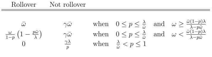
A retail bank’s payoff (to rolling over or not) depends on a wholesale bank’s realized

idiosyncratic productivity and on the actions of other retail banks. These payoffs are derived

in Appendix A.2 and given in Table 3, where 1−pt is the proportion of retail banks that

rollover. γ is the productivity of the retail bank (i.e. the retail banks’ equivalent of ωwt)

and measures the retail banks’ ability to do a wholesale bank’s job. When γ = 0, retail and wholesale banks are complements in the financial sector—neither can do the others’ job.

return from capital management.12

Table 3: Payoffs to retail banks

Rollover Not rollover

¯

ω γω¯ when 0≤p≤ λ ¯

ω and ω ≥

¯ ω(1−p)λ

λ−pω¯ ω

1−p 1− pω¯

λ

γω¯ when 0≤p≤ λ ¯

ω and ω < ¯ ω(1−p)λ

λ−pω¯

0 γλ_p when _ωλ_¯ < p≤1

Note: Payoffs are normalized byRK,tQt−1Kwt−1, and are for a given retail bank’s

action regarding a given wholesale bank. Since the problem is a static, symmetric game, all time and bank indexes have been dropped.

Table 3, top-left: When the fraction of retail banks not rolling over, pt, is low and the

wholesale bank’s productivity, ωwt, is high, a retail bank that rolls over receives the

non-default return ¯ωt. Bottom-left: If however, the retail bank rolls over when a large fraction of

retail banks do not, such that the wholesale bank runs out of capital, the rolled over retail

bank gets zero. Middle-left: This is the intermediate outcome in which the wholesale bank

survives the intra-period stage but cannot fully repay its debt obligation at the end of t. The right column gives the payoffs from not rolling over. If a retail bank does not

rollover, but few other retail banks do likewise so the wholesale bank does not lose all its

capital, the retail bank receives ¯ωt, applies its own productivity, γ, and earns γω¯t.

Right-bottom: If the fraction of retail banks that do not rollover is high, the wholesale bank has

insufficient liquid capital and the liquid capital, λt, is divided equally among the retail banks

that do not roll over, earning γλt/pt.

The payoff structure exhibitsstrategic complementarities. Up to the criticalptat which

the wholesale bank fails (i.e. runs out of capital), thenetpayoff from rolling over (i.e. rollover minus not rolling over) decreases as the fraction of retail banks that do not rollover, pt, rises.

Thus, retail banks face a strategic environment in which higher-order beliefs regarding the

actions of other retail banks are important.

Proposition 1 states that, under certain technical assumptions, a retail bank’s action is

uniquely determined by its signal: It only rolls over if its signal, ωrwt, is above a threshold,

denoted ω∗_t.

Proposition 1 There is a unique (symmetric) equilibrium in which a retail banks does not rollover if it observes a signal ωrwt below threshold ωt∗, and rolls over otherwise.

12_{Whenγ is sufficiently high, retail banks will have no incentive to lend to wholesale banks since they will}

The proof is given in Appendix A.2.13 In computing the threshold, ω_t∗, observe that a retail bank with signalωrwt =ωt∗, must be indifferent between rolling over and not. The retail

bank’s posterior distribution of ωwt is uniform over the interval [ωt∗−ε, ωt∗+ε]. Moreover,

the retail bank believes that the fraction of retail banks not rolling over, pt, is given by

p(ωw, ω∗) =

    

1 ω∗−εrw > ωw 1

2 + ω∗_−ω

w

2εrw if ω ∗_−ε

rw ≤ ωw ≤ ω∗+εrw

0 ωw < ω∗+εrw

.

Thus, the posterior distribution of pt is uniform over [0,1]. In the limit when ¯ε → 0 the

resulting indifference condition is given by14

Z 1

p=λ_¯ω

−γλ

p dp+

Z λ_¯ω

p=0

ω∗

1−p

1− pω¯

λ

−γω¯

dp= 0. (12)

where solving for ω_t∗ leads to Proposition 2.

Proposition 2 In equilibrium, with the noise component of retail banks’ signals arbitrarily close to zero, the rollover threshold, ω∗_t, is given by

ω_t∗ =γλtxt(1−ln (xt)) (xt+ (1−xt) ln (1−xt)) −1

, (13)

where xt≡λt/ω¯t. It is a striking result of Proposition 1 that there exists a unique switching

equilibrium, even when the noise term in retail banks’ signals is arbitrarily close to zero. Thus,

in equilibrium, wholesale banks never experience a partial run but experience a complete run

and full rollover with probability F (ω_t∗) and 1−F(ω_t∗), respectively.

To see the inefficiency created by the coordination problem, consider the decision of a

retail bank when it is the sole holder of a wholesale bank’s debt (or, equivalently, a scenario in which retail banks can costlessly and credibly coordinate their actions).15 _{If it does not}

13_{The proof requires that there exist lower and upper dominance regions,}

0, ωLand ωH,∞

, in which a retail bank would not rollover and rollover, respectively, regardless the actions of other retail banks. This requirement is discussed in Appendix A.2. When retail banks receive a noiseless signal on the interval

ωL, ωH, there are multiple equilibria. But, a grain of doubt for retail banks (i.e. ¯εarbitrarily close to zero) leads to the starkly different (and very useful) result given in Proposition 1.

14_{This condition specifiesω}∗_forω∗_{<ω¯. The complete indifference condition is given in Appendix A.2.}

15_{There are two benchmarks against which to gauge the inefficiency. The first, applied in the text, is to}

assume that creditors can perfectly coordinate their actions. The second is to assume long-term debt. This eliminates the rollover decision and thus eliminates the coordination problem. A standard RBC model is akin to this second benchmark. Under the first benchmark, it is efficient to coordinate and not rollover for wholesale banks with extremely low values of ωwt (i.e. ωeff∗ >0). Even after accounting for the liquidation

rollover it gets γλt and if it rolls over it gets the lesser of ¯ωt and ωwt. The optimal action

is to rollover when ωwt > γλt and not rollover otherwise. The efficient, full coordination,

threshold is given by ω_eff∗ =γλt and is lower thanωt∗, implying that, because of coordination

problems, the probability of a run is higher than is optimal. This leads to Propositions 3.

Proposition 3 i) The inefficiency wedge, ω∗/ω_eff∗ , is increasing in the illiquidity, x= λ/ω¯, of the wholesale bank: ∂(ω∗/ω_eff∗ )/∂x < 0. ii) In the limit, when the wholesale bank is not illiquid, there is no inefficiency: limx→1(ω∗/ω∗_eff) = 1.

To get a sense of the dynamic implications, suppose the loan rate (and thus ¯ωt) moves

countercyclically. This implies that in a recession, for a given λt, the distortionary effects of

coordination problems in the credit market are magnified, generating a financial accelerator.

The contracting problem A debt contract can be characterized by the pair {`t,ω¯t+1}.

Since retail banks are perfectly competitive and pay a predetermined return to depositors,

Rt, the debt contract must satisfy a zero profit break-even condition for the retail banks.

And since retail banks hold fully diversified portfolios of loans, a retail bank’s expected

(normalized) payoff is given by

¯

ω

Z ∞

¯ ω

f(ω)dω

| {z }

i. Rolled over and pay in full

+ Z ω¯

ω∗

ωf (ω)dω

| {z }

ii. Rolled over and default

+γλt

Z ω∗

0

f(ω)dω

| {z }

iii. Not rolled over

, (14)

which is an integral over three possible outcomes:16 _{The wholesale bank i) survives the}

intra-period stage and repays its loan in full; ii) survives the intra-intra-period stage but is insolvent

resulting in partial payment; or iii) does not survive and the the retail banks earn a return

managing the capital themselves. We can rewrite (14) as Γt−Gt where

Γ≡ω¯ Z ∞

¯ ω

f(ω)dω+ Z ω¯

0

ωf(ω)dω and G≡

Z ω∗ 0

(ω−γλt)f(ω)dω. (15)

Thus, 1−Γt and Γt−Gt are the fraction of gross returns accruing to wholesale and retail

banks, respectively, whereGtcaptures the deadweight loss resulting from coordination failure.

The contracting problem maximizes the wholesale banks’ return subject to the retail

banks’ break even condition, given by

max

`t,ω¯t+1

Et(1−Γt+1)St+1`t s.t. (Γt+1−Gt+1)St+1`t ≥(`t−1), (16)

contracts, but long-term contracts are preferred to short-term contracts without coordination.

16_{This assumesω}∗

where St ≡ RK,t/Rt−1. The constraint holds for all realizations of RK,t+1 because the retail

banks’ return, Rt, is assumed to be predetermined. The combined first-order condition

(substituting out the Lagrange multiplier) is given by

Et

dΓt+1

dΓt+1−dGt+1

=_Et

St+1

1 + Γt+1dGt+1−dΓt+1Gt+1

dΓt+1−dGt+1

, (17)

wheredΓt ≡∂Γt/∂ω¯t anddGt ≡∂Gt/∂ω¯t. The break-even condition from (16) and equation

(17) combine to implicitly define a loan supply schedule that has the following form

EtSt+1 =θ `t (+)

, λt −

!

, (18)

where _EtSt+1 is denoted the illiquidity premium. The illiquidity premium is increasing in

wholesale banks’ leverage and decreasing in the intra-period liquidity of capital. Endogenous

fluctuations in leverage and exogenous fluctuations in liquidity generate a time-varying wedge

between the expected return on capital and the risk-free rate in the economy.

2.5

Closing the model

Aggregation is straightforward since, at the end of a period, wholesale banks are only

het-erogenous in net worth but choose a common leverage ratio and face the same interest rate

on loans. Net worth of wholesale banks are its end-of-period profits. A fraction 1−υ of wholesale banks are the forced to exit the market and consume their profits while a measure

1−υ of new wholesale banks enter. In addition, all wholesale banks receive a positive but arbitrarily small lump-sum tranfer from households. These two assumptions ensure that i)

wholesale banks do not accumulate sufficient net worth to no longer need external finance

and ii) the net worth of every wholesale bank is positive and the contracting problem is well

defined. It follows that the evolution of aggregate net worth, Nt, is given by

Nt=υ((1−Gt)St`t−1−(`t−1−1))Rt−1Nt−1. (19)

The deadweight cost of coordination failure is in units of capital. Thus, while the aggregate

stock of capital purchased in t−1 for use in t is Kt−1, only K_t∗ = (1−Gt)Kt−1 is put to

productive use. Aggregate wholesale bank consumption of exiting bankers is given byCW,t= 1−υ

3

Results

3.1

Comparative statics

This section analyzes the comparative static properties of the static coordination failure

model. In particular, it shows the interplay between liquidity, coordination problems, leverage

and the illiquidity premium before the full dynamic properties of the model are explored.

In the next subsection, the full model is carefully parameterized to capture moments

in US aggregate data. For the present comparative static exercises, the following stylized

parameterization is used: γ =λ= 0.4, ¯ω = 0.5, andσ2 = 0.35, where ln (ω)∼N −1 2σ

2_{, σ}2 .

These parameter values aid graphical illustration without altering the qualitative properties

of the quantitatively parameterized model presented in the next section.

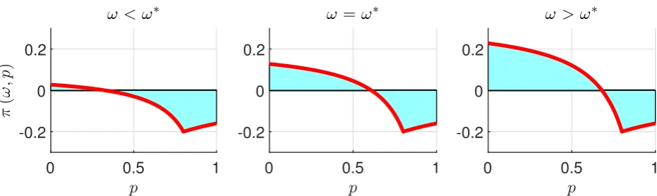
Figure 1: Net payoff function

0 0.5 1

-0.2 0 0.2

0 0.5 1

-0.2 0 0.2

0 0.5 1

-0.2 0 0.2

Note: Setγ=λ= 0.4 and ¯ω= 0.5. This givesω∗ = 0.3275. The left and right panels setω=ω∗±0.1. ω∗ is the value of ωthat equalized the shaded area above and below the line.

The red line in Figure 1 plots the net payoff function to rolling over for variousωvalues. The payoff function exhibits two important features: A single crossing where the net payoff

to rolling over is zero, and a negative slope, which implies strategic complementarities. In the

left-panel (low ω), the equilibrium action is to not rollover whereas in the right-panel (high

ω), the equilibrium action is to rollover. The middle panel defines the threshold ω∗ (solving the indifference condition in (12)), which is when the sum of the blue areas equals zero.

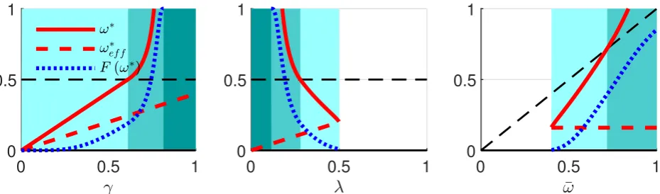
Figure 2 plots the behaviour of ω∗ and ω∗_eff as γ, λ, and ¯ω are altered, respectively. In Section 2, I focused the model’s derivation on a specific region of the parameter space,

which I term the mild fragility scenario. However, as Appendix A.2 describes in detail, the model generates four scenarios: 1) No fragility, 2) Mild fragility, 3) Acute fragility, and 4)

No rollover. These are represented in Figure 2 by the shaded areas from white to dark green,

Figure 2: Comparative statics for ω∗

0 0.5 1

0 0.5 1

0 0.5 1

0 0.5 1

0 0.5 1

0 0.5 1

Note: Set γ =λ= 0.4 and ¯ω = 0.5. The shaded areas from white to dark-green represent Scenario 1) No fragility; 2) Mild fragility; 3) Acute fragility; and 4) No rollover.

coordination problem: Retail banks base their rollover decision on their private signal alone

and not on higher order beliefs about other retail banks’ actions. The pale green region is

the mild fragility scenario that is the focus of this paper. In this scenario, ω∗ <ω¯. A fall in liquidity, (i.e. a lowering of λ) raises the rollover threshold and lowers the efficient rollover threshold, thus increasing the inefficiency generated by the coordination problem. When λ

falls further, the economy enters the acute fragility scenario in which ω∗ > ω¯. Notice the curvature of the red line. In this scenario, the rollover threshold becomes very sensitive to

small changes in liquidity. And, as a result, the proportion of wholesale banks that experience

a run, F (ω∗), also increases dramatically (blue-dot line). Finally, when the liquidity of the capital stock is extremely low, there is a no rollover scenario, in which case rollover never

occurs and the market effectively fails to exist. Clearly, there are interesting nonlinearities

in this model, but which are beyond the scope of the current paper to explore further. This paper focuses on perturbations of the model in the light-green (mild fragility) region. One

can think of the model of Gertler and Kiyotaki (2015) and Gertler et al. (2016) as studying

large jumps from the white (no fragility) region to the dark-green (no rollover) region.

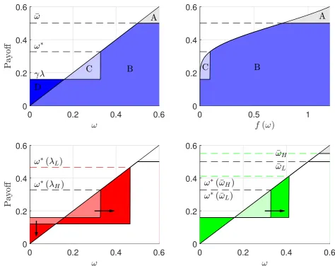
Figure 3 plots the debt contract, showing how the return on capital is split between

the borrower and creditor for different realizations of the wholesale bank’s idiosyncratic ω. Top-left panel: A textbook debt contract has the creditor receiving the area Γ (·) = B +C

Figure 3: Debt contract

0 0.2 0.4 0.6

0 0.2 0.4 0.6

0 0.5 1

0 0.2 0.4 0.6

0 0.2 0.4 0.6

0 0.2 0.4 0.6

0 0.2 0.4 0.6

0 0.2 0.4 0.6

Note: Top-left: Γ (·) =B+Cand 1−Γ (·) =A. Deadweight cost given byG(·) =C−D. Top-right panel is probability-weighted. Bottom-left: Comparative static of a rise in illiquidity (i.e. fall in λfrom λH to λL).

The deadweight cost rises (i.e. areaC−D expands). Bottom-right: Comparative static of a rise in ¯ω from ¯

ωLto ¯ωH. The deadweight cost again increases.

long-term. The top-right panel shows the same panel but probability-weighted and shows that, given the distributional assumptions, area Dis negligible. The bottom-left panel shows the effect of a rise in illiquidity caused by a fall in λ from 0.4 to 0.3. As a result, ω∗ rises and the deadweight cost rises (i.e. the area C−D expands). The bottom-right panel shows the effect of an exogenous rise in the lending rate, with ¯ω rising from 0.5 to 0.55. This also increases ω∗ and the deadweight cost of coordination failure.

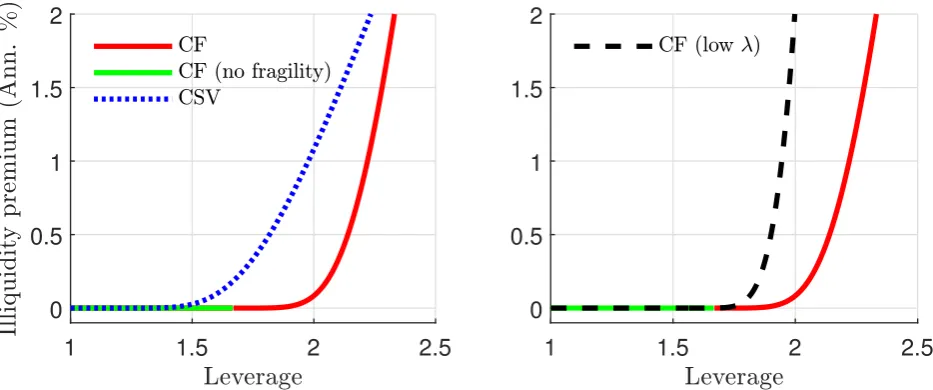
Figure 4 plots the supply curve of loanable funds by translating the deadweight costs

of coordination failure studied above into a tradeoff between wholesale banks’ leverage and

Figure 4: Illiquidity premium and leverage

1 1.5 2 2.5

0 0.5 1 1.5 2

1 1.5 2 2.5

0 0.5 1 1.5 2

Note: Set γ =λ= 0.4, ¯ω = 0.5 and σ= 0.35. CF denoted coordination failure model. CSV denotes the costly state verification model of Bernanke et al. (1999) with monitoring cost parameterµ= 0.166.

left panel shows that if wholesale banks have low leverage (green line), then there is no

coordination problem for retail banks and as a result the illiquidity premium is zero. However,

as leverage rises above a critical value then the coordination problem appears (red line),

generating an illiquidity premium which is increasing in leverage. An interesting comparison

is with an alternative model of financial frictions, the costly state verification (CSV) model

of Townsend (1979). In this model, costly state verification generates a risk premium even for low levels of leverage but grows more gradually (blue-dot line). The implication of this

comparison is that the CSV-type risk premium is larger during normal times (when leverage

is relatively low) than the CF-type illiquidity premium, but in periods of financial stress when borrower net worth falls and leverage sharply rises, then illiquidity premium rise rapidly and

can even become larger than typical risk premia.

The right panel shows the effect of a fall in liquidity. When λ falls, the loanable funds supply schedule shifts inward and steepens, resulting in a higher illiquidity premium for a

given leverage ratio. The next section studies the dynamic effect of such an illiquidity shock.

3.2

Parameterization

Table 4 list the calibrated and estimated parameters. The model parameters are partitioned

into three groups. The first group of parameters are results from previous studies. The

second group are calibrated using steady state relationships.

Table 4: Structural parameters

α 0.33 χ 5.02‡ σa 0.0055† υ 0.981‡

β 0.99 ρ 3 ρa 0.868† σ2 0.048‡

δ 0.025 ϕ 0.273† σλ 0.0041† γ 0.589‡

σC 2.0 ρλ 0.893† λ 0.703‡

Note: Parameters with‡are calibrated to match steady state moments. Parameters with†

are estimated using simulated method of moments to match US aggregate data moments.

parameters are chosen to minimize the distance between the model moments and moments

in US aggregate data. Formerly, the estimator is the solution of the following problem

J = min

θ M

D₋

M(θ)0W−1 MD−M(θ), (20)

where MD _{denotes a vector that comprises the unconditional variances and autocorrelations}

of output, consumption, investment, hours worked and the illiquidity premium in the data

and M(θ) denotes its model counterpart and θ={ϕ, σa, ρa, σλ, ρλ}. W is a diagonal matrix

that contains the standard errors of the data moment estimates.

Based on standard values in the literature at a quarterly frequency, the subjective

discount factor is β = 0.99, the intertemporal elasticity of substitution, 1/σC = 2.0, the

inverse of the Frisch elasticity of labor supply is ρ= 3 and the depreciation rate of capital is 0.025. The weight on leisure in the utility function, χ is chosen such that steady state labor supply is normalized to 1.

The financial sector is governed by four structural parameters: The capital

manage-ment productivity of retail banks,γ, the steady-state intra-period liquidity of capital,λ, the variance of the distribution of idiosyncratic shocks,σ2_{, and the proportion of wholesale banks}

that survive each period, υ. The values are pinned down by four steady state moments of the model that approximately match long-run averages in US data, given in Table 5.

One, I use the TED spread, which is the spread between the 3-month LIBOR and the

3-month Treasury bill, as a proxy for the illiquidity premium. LIBOR is the rate banks charge each other for lending. Since the coordination problem in the lending relationship between

retail and wholesale banks is the only wedge between the return on deposits and the return

on capital in this model, the TED spread is a good proxy for the illiquidity premium. For

comparison, Figure 5 plots the TED spread alongside the Gilchrist and Zakrajsek (2012a)

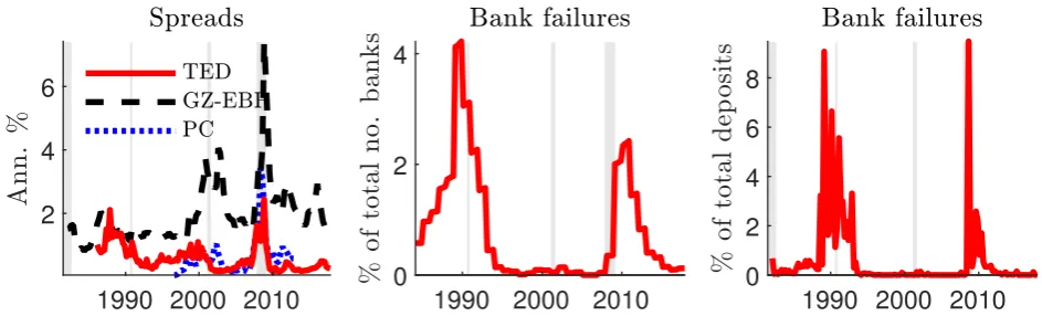
Figure 5: Illiquidity premium and bank failure

1990 2000 2010 2

4 6

1990 2000 2010

0 2 4

1990 2000 2010 0

2 4 6 8

Note: TED is the spread between 3-month LIBOR and the 3-month Treasury bill. GZ-EBP is the excess bond premium from Gilchrist and Zakrajsek (2012a). PC is a liquidity premium calculated from 7 spread series using principal components analysis following Bredemeier et al. (2018). Bank failure source: FDIC. Shaded areas denote NBER recession dates.

of credit spreads/risk premiums. The figure also plots an alternative measure of the

liquid-ity premium, which takes the principal component of seven spreads between the return on

Treasuries and illiquid assets of similar safety and maturity. This follows the methodology

of Bredemeier et al. (2018) (see Appendix C for details).17 _{Thus, I match the steady state}

illiquidity premium to the mean of the TED spread from 1986-2017, which is 58bp.

Two, Figure 5 also plots a time-series of bank failures, which I constructed from FDIC

data. The series goes back to 1934 but for consistency with the other time-series, I use

only the period 1986-2017. In the model, the fraction of banks that fail and the fraction of

failures weighted by balance sheet size are equivalent. In the data, however, these series are quite different. In particular, at the peak of the 2007-08 financial crisis, 2% of banks covered

by the FDIC failed but this accounted for 9% of total deposits. In addition, there were a

large number of bank failures in the aftermath of the crisis in 2010-12 but these were mainly

small banks. Thus, the series for bank failures in terms of total deposits appears much less

persistent. For the empirical exercise, I use the measure of bank failures and as a share of

deposits. The mean annualized failure rate from 1986-2017 was 0.67%.

Three, leverage in the wholesale bank sector varies widely across financial institutions,

with some banks with leverage in excess of 10. I take a conservative estimate and calibrate

the steady state leverage of the wholesale bank sector to be 4 following Gertler et al. (2012).18

17_{Robustness exercises using this series are available on request.}

18_{While the deterministic steady state is, by definition, independent of uncertainty, it is likely that wholesale}

Finally, the average recovery ratio of liquidated assets is set at 50% following estimates from

Berger et al. (1996).

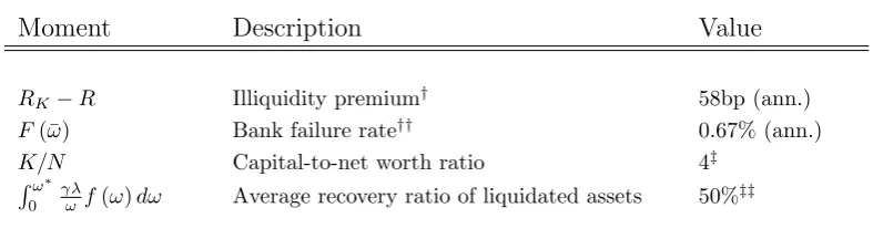
Table 5: Targeted steady state moments

Moment Description Value

RK−R Illiquidity premium† 58bp (ann.)

F(¯ω) Bank failure rate†† 0.67% (ann.)

K/N Capital-to-net worth ratio 4‡

Rω∗

0

γλ

ωf(ω)dω Average recovery ratio of liquidated assets 50%

‡‡

Note: †TED spread;††source: FDIC;‡Gertler et al. (2012). ‡‡Berger et al. (1996).

The remaining five parameters are estimated using simulated method of moments. The

following 10 moments are included: The standard deviation and autocorrelation of output,

consumption, investment, hours, and the TED spread. Four of the five parameters are the

persistence and standard deviation of the two exogenous shock series: Technology, At, and

liquidity, λt. The final parameter, ϕ, controls investment-adjustments costs. This is a key

parameter for determining the strength of the financial accelerator. When ϕ is zero, the financial accelerator is generally weak because investment demand adjusts rapidly to changes

in financial conditions.19 The success of the model in matching the business cycle moments is reported in Table 6. Given the parsimony of the model, it does a reasonable job of matching

business cycle moments. Most notably, hours worked are too volatilite and consumption is

too persistent. However, the model captures well the properties of the TED spread.

3.3

Impulse responses and crisis scenario

Technology shocks Figure 6 shows the reaction to a 1% negative technology shock.20 _The

blue-solid and green-dot lines show the reaction of the model with and without coordination

failure, respectively. Coordination failure does not significantly alter the qualitative shapes

of the responses, but does alter the magnitude of the responses. Notably, the drops in

investment, asset prices and the capital stock are magnified.

19_{The model is solved to first-order in the neighborhood of the deterministic steady state. The model,}

however, admits interesting non-linearities as shown in Section 3. Although it would be a fruitful avenue for future research to solve the model using global methods, it is beyond the scope of the current paper.

20_{Supplementary material on other shocks (e.g. capital quality and net worth shocks) and the behaviour}

Table 6: Business cycle moments

Moment Data Model Moment Data Model

std(GDP) 1.060 1.051 ac(GDP) 0.862 0.786

std(C) 0.864 0.686 ac(C) 0.820 0.965

std(I) 4.418 4.154 ac(I) 0.931 0.714

std(Hours) 0.478 0.794 ac(Hours) 0.792 0.676

std(TED) 0.410 0.359 ac(TED) 0.796 0.651

Note: Construction of data moments given in Appendix C.

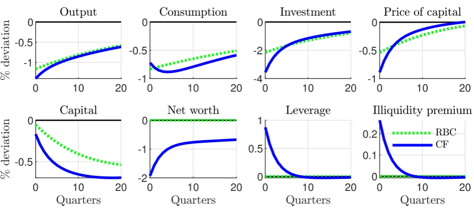
Figure 6: Technology shock

0 10 20

-1 -0.5 0

0 10 20

-1 -0.5 0

0 10 20

-4 -2 0

0 10 20

-1 -0.5 0

0 10 20

-0.5 0

0 10 20

-2 -1 0

0 10 20

0 0.5 1

0 10 20

0 0.1 0.2

Note: 1% negative technology shock

Coordination failure introduces three new aggregate variables of interest: Wholesale bank net worth and leverage and the illiquidity premium. The negative technology shock

causes a drop in wholesale bank net worth and an increase in wholesale bank leverage. The

risk-free (deposit) rate falls while the expected return on capital rises, leading to a sharp rise

in the illiquidity premium.21 _{These responses are the result of three features of coordination}

21_{The countercyclical leverage ratio is a feature of most financial accelerator models. Adrian et al. (2013)}

failure. First, the loan rate paid by wholesale banks is a function of the expected return

on capital, which means that the wholesale banks absorb the aggregate risk. When the

negative technology shock hits, the realized return on capital is below its expected return, which drives down the aggregate wholesale bank profits and hence their net worth. Second,

wholesale bank net worth decreases faster than the demand for capital, implicitly causing

leverage to rise. Third, higher leverage increases the severity of the coordination problem

among retail banks, causing the illiquidity premium to rise. As a result, retail banks demand

a higher loan rate (i.e. an increase in ¯ωt) following a negative productivity shock, which

increases the illiquidity of wholesale banks yet further. This causes investment and the price

of capital to fall further in response to a negative technology shock. Investment falls 3.8%

on impact following a 1% technology shock in the coordination failure model, relative to a

2.0% in the frictionless case.

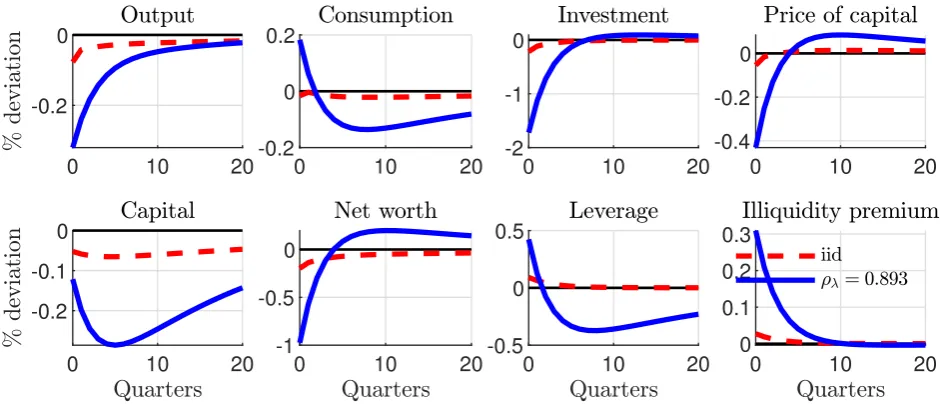
Illiquidity shock A novel feature of the model is the ability to generate an exogenous

rise in illiquidity in credit markets. Figure 7 shows the response to a 1% rise in intra-period

capital illiquidity with an iid (red-dash) and a persistent shock (blue-solid line), respectively.

Figure 7: Illiquidity shock

0 10 20

-0.2 0

0 10 20

-0.2 0 0.2

0 10 20

-2 -1 0

0 10 20

-0.4 -0.2 0

0 10 20

-0.2 -0.1 0

0 10 20

-1 -0.5 0

0 10 20

-0.5 0 0.5

0 10 20

0 0.1 0.2 0.3

Note: 1% illiquidity shock

A rise in the illiquidity of capital leads to a rise in the rollover threshold,ω∗, implying a higher incidence of bank runs. This causes a sharp rise in the illiquidity premium paid by

wholesale banks on external finance. The rise in the illiquidity premium is the result of both

a rise in the expected return on capital as well as a fall in the risk-free deposit rate. The

capital is insufficient to offset the fall in wholesale bank net worth. In order to break even,

the retail banks lower the return paid on deposits. Households, facing a lower return on

savings, generates a temporary consumption boom.22 In the transition back to steady state, the fall in the demand for investment causes a decline in the capital stock. As the impact of

the illiquidity shocks recedes, households cut consumption order to restore their steady state

savings ratio. This requires a long period of deleveraging by wholesale banks.

The size and persistence in the response of capital (and hence output) is sensitive to

the persistence of the exogenous rise in illiquidity. The evolution of capital is relatively

gradual. A less persistent shock therefore gives less opportunity for capital to fall and do

serious damage to potential output. Thus, the length and severity of a recession depends on

how long the credit market remains illiquid.

This model has several features unique to coordination failure. First, retail banks’ are most likely to run when liquidity is most needed. Second, as the constraints on wholesale

banks tighten countercyclically, the share of capital held by retail banks will move

counter-cyclically. This occurred during the financial crisis with dealer banks in the shadow banking

sector shrinking and commercial banks expanding their market share.

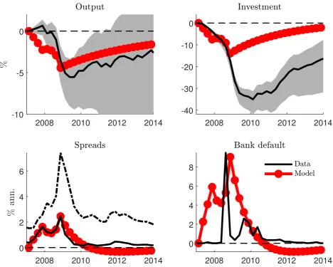
Illiquidity during the 2007-08 financial crisis In this section, I provide an illiquidity

shock narrative of the 2007-08 financial crisis as an external validation exercise for the model.

Since the model is a parsimonous RBC model, chosen for clarity rather than quantitative

accuracy, it is unlikely to provide a close fit to the data. However, the exercise provides a

good way of assessing its strengths and weaknesses.

In this exercise, I suppose the economy was hit by a sequence of illiquidity shocks from

2007q2–2008q4 that match the evolution of the illiquidity premium (TED spread) in the

data. Using simple projection methods, I estimate a distribution of counterfactual paths

for output, investment, the illiquidity premium and bank failure had the financial crisis not

occurred. The black line in Figure 8 represents the deviation between the actual path for these

variables and the median of the counterfactual path. The methodology follows Christiano et

al. (2015) and is described in Appendix C. The grey area captures the uncertainty in these

counterfactual paths. The counterfactual evolution of output is most uncertain while the

bank failure rate is estimated very precisely (i.e. without the financial crisis, the bank failure rate would have almost certainly remained at zero).

22_{The implication is that when an illiquidity shocks hits, consumption rises temporarily while output and}

Figure 8: Illiquidity shocks during the 2007-08 crisis

2008 2010 2012 2014

-10 -5 0

2008 2010 2012 2014

-40 -30 -20 -10 0

2008 2010 2012 2014

0 2 4 6

2008 2010 2012 2014

0 2 4 6 8

Note: Black lines represent the data relative to an uncertain trend using following Christiano et al. (2015). Black-dash line is the Gilchrist and Zakrajsek (2012b) EBP. Red line is the model prediction with illiquidity shocks chosen to match exactly the TED spread from 2007q2–2008q4.

The model’s illiquidity shocks captures well the fall in output during the financial crisis although only around a third of the drop in investment, suggesting that investment specific

shocks also played an important role. The model captures well the peak bank failure rate of

9%. However, the model predicts that bank failures would have appeared as early as 2007

and would have persisted into 2010. Thus, when integrating over the total number of bank

failures for the 2007-2010 period, the model overpredicts the number of bank failures.

Of course, there is a clear rationale for policymakers (monetary or fiscal) to offset the

4

Policy responses

The coordination failure model facilitates the analysis of two unconventional credit market policies adopted by the US Federal Reserve during the 2007-08 financial crisis: 1) Direct

lending (or liquidity injections) in credit markets and 2) equity injections.23

4.1

Direct lending (DL)

In this scenario, the policymaker supplements private lending in credit markets with

addi-tional lending directly to wholesale banks with abnormal excess returns. Since wholesale

banks in the model are funded by a continuum of retail banks, the retail banks cannot

coor-dinate actions. The policymaker instead behaves as a single, large market participant with

deep pockets. By committing to rollover, it is able to reduce the coordination problem.24

Let nt denote the proportion of total lending to wholesale bank w provided by retail

banks. Funding provided by the policymaker is therefore given by (1−nt) (QtKwt−Nwt).

Retail banks can still choose not to rollover while the policymaker is assumed to always

rollover.25 _{The policymaker lends at the prevailing market rateR}

L,t. However, by expanding

the supply of run-free funds available in the market, it reduces the loan rate endogenously.

The new rollover threshold, augmented by direct lending, is given by

ω∗ =γλnx(1−ln (x))/(nx+ (1−nx) ln (1−nx)), (21)

wherex≡λ/(nω¯) is the new measure of endogenous illiquidity. The efficient rollover thresh-old becomes ω_eff∗ = γλ/n. It is straightforward to show that, all else equal, direct lending increases the efficient threshold while ω∗ falls, thus reducing the market distortion.26 _Retail

banks’ break-even condition is unchanged except for the deadweight cost, Gt, given by

G= Z ω∗

0

(ω−γλ/n)f(ω)dω. (22)

23_{C´urdia and Woodford (2010), Reis (2009a) and Gertler and Kiyotaki (2010) also model the effect of}

credit market policies.

24_{In other respects, the government is likely less efficient at intermediating funds. Thus, think of this as}

only a crisis measure.

25_{In the crisis, the Fed implicitly lengthened the maturity structure of banks’ borrowing by directly}

lending at longer maturities than private agents were willing to lend. See the Fed’s press release: http://www.federalreserve.gov/newsevents/press/monetary/20081007c.htm

26_{In fact, a sufficiently large intervention will push the economy into the “no fragility” region described in}

4.2

Equity injections (EI)

In this scenario, the policymaker acquires part ownership of wholesale banks.27 _{I assume that}

government equity and private equity has the same characteristics. Let ct be the proportion

of total equity that is privately held by wholesale bankers, such that the funds injected by the

government are given by (1−ct)Nt. The retail banks’ break-even condition is unchanged

but wholesale bank profits are split between the wholesale bankers and the government in

proportion to ct. The augment net worth equation is given by

Nt =

ct−1

ct

υ((1−Gt)St`t−1−(`t−1−1))Rt−1Nt−1.

Since equity injections expand wholesale bank net worth, this will expand credit creation,

reduce leverage ratios, and lower the illiquidity premium.

4.3

The policy rule

The policymaker obtains funds by levying lump sum taxes on households.28 _{Returns from}

direct lending and equity are also transferred lump sum to households. The aim is to assess

the relative power of the two alternative instruments and so this simplification facilitates a

clean comparison. The government flow budget constraint is given by

Tt= (1−nt−1)

Γt−

Z ω_t∗

0

ωf(ω)dω

RK,tQt−1Kt−1

| {z }

Return on direct lending

+ (1−ct−1) (1−Γt)RK,tQt−1Kt−1

| {z }

Return on equity injections

−(1−nt) (QtKt−Nt)

| {z }

Direct lending

− (1−ct)Nt

| {z }

Equity injections

, (23)

where Tt are lump-sum transfers net of taxes. Note the policymaker does not receive the

same return on direct lending as retail banks. Since the policymaker commits to always

rollover, it loses γλt to banks that still experience a run.

The policymaker has two policy instruments available, ct and nt. I consider a simple

and implementable reaction function that governs the use of these instruments given by

nt= 1−aDL(EtSt+1/S−1) and ct= 1−aEI(EtSt+1/S−1), (24)

27_{I abstract from efficiency costs associated with government acquisition of equity}

28_{The lump sum taxes/transfers should more realistically be modelled as central bank reserves when}

where aDL, aEI ≥0. Thus, the size of the policy intervention depends positively on the

illiq-uidity premium. The rule is reasonable since the magnitude of the distortion the policymaker

is trying to offset is proxied by the illiquidity premium. The rule is also practically imple-mentable since credit spreads are observable (although disentangling illiquidity risk from

credit risk may not be so easy). After all, it was the sharp rise in spreads during the financial

crisis that pushed the Fed into introducing unconventional credit policies, even before the

conventional tool of monetary policy, the nominal interest rate, reached the zero lower bound.

4.4

Illiquidity shock with policy responses

Figure 9 shows a 1% fall in the intra-period liquidity of the capital stock. To provide a clear

comparison between policy instruments, the experiment ensures that both policies deliver

the same initial cost to the government in term of GDP. This requires the parameters of the policy rules to be set at aDL = 3.00 andaEI = 14.02.29

Figure 9 shows that equity injections mitigate the effects of the initial shock to liquidity

better than direct lending. The initial fall in output with no policy intervention was 0.35%.

Equity injections and direct lending reduced this to 0.11% and 0.27%, respectively. The

reason is that equity injections directly offset the fall in net worth, actually causing leverage

to fall. However, while equity injections reduce the initial impact of the illiquidity shock, they

also cause the effects of the shock to persist for longer. The reason is as follows: Without

coordination problems, the Modigliani-Miller theorem states the irrelevance between debt

or equity financing. But, with coordination problems, the shadow price of equity is lower, exactly because equity avoids the coordination problem. Wholesale banks build up equity

so that they don’t require debt finance. Direct lending, even though it reduces the maturity

mismatch, does not materially improve the solvency of the wholesale banks. Equity injections

are therefore powerful in mitigating the problem in credit markets (because it lowers the need

to access them). However, as the illiquidity premium recedes, the policymaker’s withdrawal

of equity offsets the recovery in net worth that the wholesale bank would have experienced

in the counterfactual scenario without policy intervention.

5

Conclusion

This paper incorporates short-term uncoordinated creditors in credit markets in a dynamic,

general equilibrium setting. The coordination problem generates a time-varying incidence of

bank runs, rising during downturns and especially during periods of illiquidity. The resulting

29_{In terms of quantities, the size of the initial intervention in these experiments is 0.6% of annual GDP, or}

Figure 9: Illiquidity shock and policy response

0 10 20

-0.2 0

0 10 20

-0.2 0 0.2

0 10 20

-2 -1 0

0 10 20

-0.4 -0.2 0

0 10 20

-0.2 -0.1 0

0 10 20

-1 -0.5 0

0 10 20

-0.5 0 0.5

0 10 20

0 0.1 0.2 0.3

Note: 1% illiquidity shock with policy intervention

illiquidity premium provides a new lense through which to study the financial accelerator

and the role of credit market interventions during financial crises. In particular, the model

shows that equity injections are more powerful policies than direct lending.

Moreover, the microfounded coordination problem at the heart of this model provides

rich nonlinearities that this current research has not yet fully explored and will likely be a

References

Adrian, Tobias, Paolo Colla, and Hyun Song Shin (2013) ‘Which financial frictions? Parsing

the evidence from the financial crisis of 2007 to 2009.’ NBER Macroeconomics Annual 27(1), 159–214

Angeloni, Ignazio, and Ester Faia (2013) ‘Capital regulation and monetary policy with fragile

banks.’ Journal of Monetary Economics60(3), 311–324

Bagehot, Walter (1873) Lombard Street: A description of the money market(London: Henry S. King & Co.)

Basu, Susanto, and Brent Bundick (2017) ‘Uncertainty shocks in a model of effective demand.’

Econometrica 85(3), 937–958

Berger, Philip G., Eli Ofek, and Itzhak Swary (1996) ‘Investor valuation of the abandonment

option.’Journal of Financial Economics 42(2), 257–287

Bernanke, Ben S., and Mark Gertler (1989) ‘Agency costs, net worth, and business

fluctua-tions.’ American Economic Review 79(1), 14–31

Bernanke, Ben S., Mark Gertler, and Simon Gilchrist (1999) ‘The financial accelerator in a

quantitative business cycle framework.’ vol. 1C of Handbook of Macroeconomics (Amster-dam: Elsevier) chapter 21, pp. 1341–1393

Bredemeier, Christian, Christoph Kaufmann, and Andreas Schabert (2018) ‘Interest rate

spreads and forward guidance’

Brunnermeier, Markus K. (2009) ‘Deciphering the liquidity and credit crunch 2007-2008.’

Journal of Economic Perspectives23(1), 77–100

Brunnermeier, Markus K., and Martin Oehmke (2013) ‘The maturity rat race.’ Journal of Finance68(2), 483–521

Carlsson, Hans, and Eric van Damme (1993) ‘Global games and equilibrium selection.’ Econo-metrica 61(5), 989–1018

Carlstrom, Charles T., and Timothy S. Fuerst (1997) ‘Agency costs, net worth, and

busi-ness fluctuations: A computable general equilibrium analysis.’American Economic Review 87(5), 893–910

Carlstrom, Charles T., Timothy S. Fuerst, and Matthias Paustian (2010) ‘Optimal monetary

(2016) ‘Optimal contracts, aggregate risk, and the financial accelerator.’ American Eco-nomic Journal: MacroecoEco-nomics 8(1), 119–47

Christiano, Lawrence J., Martin S. Eichenbaum, and Mathias Trabandt (2015)

‘Understand-ing the great recession.’American Economic Journal: Macroeconomics 7(1), 110–67

Christiano, Lawrence J., Roberto Motto, and Massimo Rostagno (2014) ‘Risk shocks.’ Amer-ican Economic Review104(1), 27–65

Corsetti, Giancarlo, Amil Dasgupta, Stephen Morris, and Hyun Song Shin (2004) ‘Does one

Soros make a difference? A theory of currency crises with large and small traders.’ Review of Economic Studies 71(1), 87–113

C´urdia, Vasco, and Michael Woodford (2010) ‘Conventional and unconventional monetary

policy.’ Federal Reserve Bank of St. Louis Review92(4), 229–64

(2016) ‘Credit frictions and optimal monetary policy.’ Journal of Monetary Economics 84, 30–65

Dang, Tri Vi, Gary Gorton, and Bengt Holmstr¨om (2012) ‘Ignorance, debt and financial

crises.’ Unpublished manuscript

de Groot, Oliver (2014) ‘The risk channel of monetary policy.’ International Journal of Cen-tral Banking10(2), 115–160

(2016) ‘The financial accelerator.’ In The New Palgrave Dictionary of Economics, ed. Steven N. Durlauf and Lawrence E. Blume (Basingstoke: Palgrave Macmillan)

Del Negro, Marco, Gauti Eggertsson, Andrea Ferrero, and Nobuhiro Kiyotaki (2017) ‘The

great escape? a quantitative evaluation of the fed’s liquidity facilities.’American Economic Review 107(3), 824–57

Diamond, Douglas W., and Philip H. Dybvig (1983) ‘Bank runs, deposit insurance, and

liquidity.’Journal of Political Economy 91(3), 401–419

Dmitriev, Mikhail, and Jonathan Hoddenbagh (2017) ‘The financial accelerator and the

optimal state-dependent contract.’ Review of Economic Dynamics24, 43–65

Fiore, Fiorella D., and Oreste Tristani (2013) ‘Optimal monetary policy in a model of the

credit channel.’The Economic Journal 123(571), 906–931

Gertler, Mark (2013) ‘Comment on “Which financial frictions? Parsing the evidence from

Gertler, Mark, and Nobuhiro Kiyotaki (2010) ‘Financial intermediation and credit policy in

business cycle analysis.’ vol. 3 ofHandbook of Monetary Economics(Amsterdam: Elsevier) chapter 11, pp. 547–599

(2015) ‘Banking, liquidity, and bank runs in an infinite horizon economy.’ American Eco-nomic Review 105(7), 2011–43

Gertler, Mark, and Peter Karadi (2011) ‘A model of unconventional monetary policy.’Journal of Monetary Economics 58(1), 17–34

Gertler, Mark, Nobuhiro Kiyotaki, and Albert Queralto (2012) ‘Financial crises, bank risk

exposure and government financial policy.’ Journal of Monetary Economics 59, Supple-ment, 17–34

Gertler, Mark, Nobuhiro Kiyotaki, and Andrea Prestipino (2016) ‘Wholesale banking and

bank runs in macroeconomic modeling of financial crises.’ vol. 2 of Handbook of Macroeco-nomics (Amsterdam: Elsevier) chapter 11, pp. 1345–1425

Gilchrist, Simon, and Egon Zakrajsek (2012a) ‘Credit spreads and business cycle

fluctua-tions.’ American Economic Review 102(4), 1692–1720

(2012b) ‘Credit spreads and business cycle fluctuations.’ The American Economic Review 102(4), 1692–1720

Goldstein, Itay, and Ady Pauzner (2005) ‘Demand–deposit contracts and the probability of bank runs.’ Journal of Finance 60(3), 1293–1327

Gorton, Gary, and Andrew Winton (2003) ‘Financial intermediation.’ vol. 1A of Handbook of the Economics of Finance: Corporate Finance(Amsterdam: Elsevier) chapter 8, pp. 431– 552

Hart, Oliver, and John Moore (1994) ‘A theory of debt based on the inalienability of human

capital.’ Quarterly Journal of Economics 109(4), 841–79

Heider, Florian, Marie Hoerova, and Cornelia Holthausen (2015) ‘Liquidity hoarding and interbank market rates: The role of counterparty risk.’ Journal of Financial Economics 118(2), 336 – 354

Hertzberg, Andrew, Jos´e M. Liberti, and Daniel Paravisini (2011) ‘Public information and

Iacoviello, Matteo (2005) ‘House prices, borrowing constraints, and monetary policy in the

business cycle.’ The American Economic Review95(3), 739–764

Jackson, Thomas H. (1986)The logic and limits of bankruptcy law(Boston: Harvard Univer-sity Press)

Kiyotaki, Nobuhiro, and John Moore (1997) ‘Credit cycles.’ Journal of Political Economy 105(2), 211–248

Krishnamurthy, Arvind, and Annette Vissing-Jorgensen (2012) ‘The aggregate demand for

treasury debt.’Journal of Political Economy 120(2), 233–267

Kurlat, Pablo (2013) ‘Lemons markets and the transmission of aggregate shocks.’ American Economic Review 103(4), 1463–1489

Morris, Stephen, and Hyun Song Shin (2003) ‘Global games: Theory and applications.’

vol. 1 of Advances in economics and econometrics: Theory and applications, Eighth world congress (Cambridge: Cambridge University Press) pp. 56–114

(2004) ‘Coordination risk and the price of debt.’ European Economic Review 48, 133–153

(2016) ‘Illiquidity component of credit risk.’ International Economic Review 57(4), 1135– 1148

Reis, Ricardo (2009a) ‘Interpreting the unconventional US monetary policy of 2007-09.’ Brookings Papers on Economic Activity pp. 119–165

(2009b) ‘Where should liquidity be injected during a financial crisis?’ Unpublished manuscript

Rochet, Jean-Charles, and Xavier Vives (2004) ‘Coordination failures and the lender of last

resort: Was Bagehot right after all?’ Journal of the European Economic Association 2(6), 1116–1147

Sargent, Thomas J., and Neil Wallace (1982) ‘The real-bills doctrine versus the quantity

theory: A reconsideration.’ Journal of Political Economy90(6), 1212–1236

Shin, Hyun Song (2009) ‘Reflections on Northern Rock: The bank run that heralded the

global financial crisis.’ Journal of Economic Perspectives23(1), 101–119

Townsend, Robert M. (1979) ‘Optimal contracts and competitive markets with costly state