Published online January 10, 2014 (http://www.sciencepublishinggroup.com/j/earth) doi: 10.11648/j.earth.20140301.11
The modification of the matrix method for the modelling
of propagation of the body waves
Anastasiia Pavlova
Carpatian Branch of the Institute of geophysics named after S.I. Subbotin NAS of Ukraine, Lviv, Ukraine
Email address:
[email protected]To cite this article:
Anastasiia Pavlova. The Modification of the Matrix Method for the Modelling of Propagation of the Body Waves. Earth Science. Vol. 3, No. 1, 2014, pp. 1-8. doi: 10.11648/j.earth.20140301.11
Abstract:
The modification of the matrix method of construction of wavefield on the free surface of an anisotropicmedium is presented. The earthquake source represented by a randomly oriented force or a seismic moment tensor is placed on an arbitrary boundary of a layered anisotropic medium. The theory of the matrix propagator in a homogeneous anisotropic medium by introducing a "wave propagator" is presented. It is shown that for anisotropic layered medium the matrix propagator can be represented by a "wave propagator" in each layer. The matrix propagator P(z,z0=0) acts on the
free surface of the layered medium and generates stress-displacement vector at depth z. The displacement field on the free surface of an anisotropic medium is obtained from the received system of equations considering the radiation condition and that the free surface is stressless. The approbation of the modification of the matrix method for isotropic and anisotropic media with TI symmetry is done. A comparative analysis of our results with the synthetic seismic records obtained by other methods and published in foreign papers is executed.
Keywords:
Matrix Propagator, Seismic Moment Tensor, Anisotropic Medium1. Introduction
With the increased resolution of seismic data, there is a growing awareness that an isotropic description of the Earth may no longer be adequate. Anisotropy appears to be a near ubiquitous property of earth materials, and its effects on seismic data must be quantified [25].
Measurements of seismic velocity in exploration geophysics from travel-times of P, SV and SH waves have disclosed that many rocks in sedimentary basins exhibit significant degrees of anisotropy.
Seismic velocity anisotropy is a widespread phenomenon in Earth materials. Until recently, seismic data could be adequately explained by assuming isotropy, so anisotropy could be largely ignored. With the increasing resolution of seismic observations, however, there is a growing awareness that the assumption of isotropy is often violated. Anisotropy has been widely detected in the crust and upper mantle and laboratory measurements imply that the phenomenon must be widespread in both crystalline and sedimentary rocks There are fundamental differences between wave propagation in isotropic and anisotropic media [12, 13]. In an isotropic medium, P-wave particle motion is normal to a wavefront so the P polarization vector
is coincident with the phase propagation vector. S motion may be in any direction orthogonal to P. In an anisotropic medium, the P polarization vector need not be coincident with the phase propagation vector, hence this phase is denoted qP for ‘quasi-P‘. Two quasi-shear polarizations form a mutually orthogonal set with qP. Thus for any particular direction of phase propagation, there are three body waves with fixed orthogonal polarizations. In general, the velocities and polarizations vary with direction of phase propagation, causing the transverse component of the wavenumber vector to be non-zero. As a consequence of this behaviour, in an anisotropic medium phase and energy-velocity vectors may diverge so that a ray may depart from the sagittal plane (the vertical plane through the, direction of phase propagation). Further, if the medium is elastic, energy and group velocity vectors will also diverge [3].
accumulated. Analytical problem solving methods are developed only for a relatively narrow range of tasks. More precise, and hence more complex mathematical models are implemented by numerical methods. The last give a solution only in certain limited areas of model medium, and this is the main drawback of numerical methods. This means that the use of numerical methods, including finite difference method [1, 17, 20, 21, 27] and finite element method [28, 30, 31, 33] for modelling of seismic wave propagation in inhomogeneous anisotropic media gives very high accuracy results, but requires a grid which covers the entire area occupied by the investigated object and a significant amount of computer resources for the solution of high-dimensional systems of algebraic equations.
Therefore, it is difficult to implement, even with the use of modern computational tools, including clusters. The matrix method is used to obtain solutions, which avoid the complicated procedures to satisfy all boundary conditions. The usefulness of solutions obtained by this method is considered in [2, 4-6]. The matrix method allows for a common approach to examine the propagation of waves in a wide class of systems. This method allows to obtain solutions in a more compact and convenient form for further analytical and numerical calculations.
In the 50's of 20th century Thomson and Haskell first proposed a method for constructing interference fields by simulation of elastic waves in layered isotropic half-space with planar boundaries [18]. The matrix method was developed in the works [7-10, 24].
The stable algorithms of seismograms calculation for all angles of seismic waves propagation is obtained. The matrix method is generalized for low-frequency waves in inhomogeneous elastic concentric cylindrical and spherical layers surrounded by an elastic medium. The concept of the characteristic matrix determined by physical parameters of the environment is developed. The matrix method is used for wave propagation in elastic, liquid and thermoelastic media. In addition, it has been generalized for the study of other processes described by linear equations. The advantage of the matrix method is the ability to compactly write matrix expressions that are useful both in analytical studies and numerical calculations.
The matrix method and its modifications are used to simulate the seismic waves propagation in isotropic and anisotropic media. This method is quite comfortable and has several advantages over other approaches. Both advantages and disadvantages of the matrix method are well described in [19, 29, 32, 34].
2. Theory
We assume the usual linear relationship between stress τij and strain ekl
k l ijkl kl ijkl ij
x
u
c
e
c
∂
∂
=
⋅
=
τ
(1)where u=(ux, uy, uz)T is displacement vector.
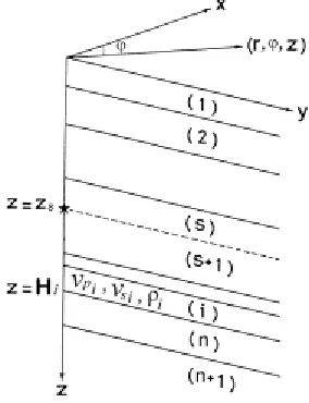
Figure 1. Model vertically inhomogeneous medium
The equation of motion for an elastic homogeneous anisotropic medium, in the absence of body forces is [15]
k i
l ijkl i
x x
u c t
u
∂ ∂
∂ = ∂
∂ 2
2 2
ρ
(2)where ρ is the uniform mass density, and
c
ijkl are theelements of the uniform elastic coefficient tensor which satisfy the symmetry conditions
klij ijlk jikl
ijkl c c c
c = = =
So that only 21 independent constants are involved. The suffixes can take the values 1, 2, or 3, and the summation convention for repeated suffixes is assumed.
Taking the Fourier transform of (1) and (2), we obtain the matrix equation [16]
) ( ) (zb z A j z b
ω
= ∂ ∂
(3)
Where =
τ
u
b is the vector of displacements and scaled
tractions, T
zz yz xz
j ( , , )
1 τ τ τ
ω
τ =− . With the definition of b
the system matrix A has the structure
=
TT
S
C
T
A
;where T, S and C are 3×3 sub matrices, C and S are symmetric.
For any vertically stratified medium, the differential system (3) can be solved subject to specified boundary conditions to obtain the response vector b at any desired depth. If the response at depth z0 is b(z0), the response at
depth z is
) ( ) , ( )
(z P z z0 b z0
Where P(z, z0) is the stress-displacement propagator. The
matrix propagator is defined as
... ) ( ) ( ) ( ) ( ) , ( 0 0 1 2 2 1 1 1 1 0 + + + + =
∫
∫
∫
z z z z d d A A A d A I z z Pξ
ξ
ξ
ξ
ξ
ξ
ξ
(4*)where I is the 6 x 6 identity.
If D is the local eigenvector matrix of A then Λ
= −AD
D 1 (5)
where Λ is diagonal. The diagonal elements of Λ are the eigenvalues of A which are the vertical phase slownessesq= pz. In general we may write
) , , , , ,
( 1 2 1 D2 s D s D p U s U s U
p q q q q q
q diag
= Λ
where superscripts U and D denote upgoing and downgoing disturbances, the subscript P denotes quasi-P and S1, S2
denote the two types of quasi-S. For an isotropic mediumqU =−qD, but for general anisotropy there is no such simple relationship between the vertical slownesses [23]. However, for our choice of Fourier transform and the definition of A in (3), and considering the radiation condition, it follows that
Im (qD) > 0 and Im (qU) < 0.
Given the eigenvector matrix D, we may define a wavevector v from the transformation
v
D
b
=
. (6)As in the isotropic case the elements of v may be identified with the amplitudes of upward and downward travelling plane waves,
T D D D u u u T D u v v
v=[ , ] =[
ϕ
,ψ
,χ
,ϕ
,ψ
,χ
] (7)where φ, denotes qP amplitude and ψ, χ the two qS amplitudes. As before U and D denote up and down.
If the elastic parameters are locally constant then D is independent of z and substitution of (6) and (5) into (3) yields v AD j z v
D = ω
∂ ∂
(8)
with the solution
)
(
)
,
(
)
(
)
(
1 1 1)
( 1
v
z
Q
z
z
v
z
e
z
v
=
jωΛ z−z⋅
=
⋅
(9)where z1 is some reference depth. From (7) it is apparent
that Q may be regarded as a 'wave propagator' since it is the solution to I z z Q z z Q j z z z
Q = Λ =
∂ ∂ ) , ( ), , ( ) , ( 1 1 1 1 ω (10)
We note from (6) that within the uniform layer, Q has the structure = D u E E z z Q 0 0 ) ,
( 1 (11)
with
]
,
,
[
],
,
,
[
( 1) ( 1) 1 ( 1) 2 ( 1) ( 1) 1 ( 1) 2D s D s D p u s u s u
p j z z q j z z q j z z q
D q z z j q z z j q z z j
u
diag
e
e
e
E
diag
e
e
e
E
=
ω − ω − ω −=
ω − ω − ω − (12)Using (6) and (9) the stress-displacement vector at any level z within the uniform medium is
) ( ) , ( ) ( 1 1 1 D b z
z z DQ z
b = − (13)
By comparison with (4) the desired propagator for the uniform interval is
1 1 1) ( , ) ,
(z z =DQ z z D−
P (14)
To find this propagator, it is necessary to find the eigenvalues (vertical slownesses), the eigenvector matrix D, and its inverse D-1. In the isotropic case these are known analytically, so the construction of the propagator is straightforward. In the anisotropic case, analytic solutions have been found only for simple symmetries so in general, solutions will be found numerically.
The layered anisotropic medium, which consists of n
homogeneous anisotropic layers on an anisotropic halfspace (n +1) (Fig. 1), is considered. The matrix propagator (4*) can be represented by a “wave propagator”
in each layer for anisotropic layered medium. The source in the form of a jump in the displacement-stress
s s b
b
F = +1− is placed on the s-boundary (Fig. 1); it is easy
to write the following matrix equation, using (13-14):
s z z s s n
n P b
b
= + +1= , 1
s z z s s s s n n n n
n D DQ D D Q D b
v = + − + + + − − +
+ = ⋅ ⋅⋅ ⋅ 1
1 1 1 1 1 1 1 1 0 1 1 1 1 1 0 0 , 1 1 , 2 2 , 1 1
, P P P b DQD DQD b
P
b ss s s s s s
z z s s ⋅ ⋅⋅ ⋅ = ⋅ ⋅⋅ ⋅ = − − − − − = F G b G F G b G G F b G G F b D Q D D Q D v s n s n s s n s s n s s s s n n n n ⋅ + = ⋅ + = + ⋅ = + ⋅ ⋅⋅ ⋅ = + + + + + + + + − + + + − + 1 , 1 0 1 , 1 0 1 ,, 1 , 1 0 1 , 1 , 1 1 1 1 1 1
1 ( ) ( )
where 1 1 1 1 1 2 1 1 1 1 1 1 1 − − − + + + − − + ⋅ ⋅⋅ ⋅ ⋅⋅
=D DQD D Q D D DQD G n n n n s s s
) ~ ( ) ( 0 ,11 0 1
1 , 0
1 Gb G G F Gb G F G b F
vn+ = + ⋅ s− ⋅ = + s− ⋅ = + (15)
where F=Gs ⋅F −1 1 , ~ , 1 , 1 , 1 s s n G G
G= + + ⋅ .
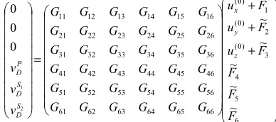
Using (15) and the radiation condition (with a halfspace (n+1) the waves are not returned), and also the fact that the tension on the free surface equals to zero, we obtain a system of equations:
+ + + = 6 5 4 3 ) 0 ( 2 ) 0 ( 1 ) 0 ( 66 65 64 63 62 61 56 55 54 53 52 51 46 45 44 43 42 41 36 35 34 33 32 31 26 25 24 23 22 21 16 15 14 13 12 11 ~ ~ ~ ~ ~ ~ 0 0 0 2 1 F F F F u F u F u G G G G G G G G G G G G G G G G G G G G G G G G G G G G G G G G G G G G v v v z y x S D S D P D
Using only the homogeneous equations is sufficient to get the displacement field on a free surface:
− = + + − = + + − = + +
∑
∑
∑
= = = 6 1 3 ) 0 ( 33 ) 0 ( 32 ) 0 ( 31 6 1 2 ) 0 ( 23 ) 0 ( 22 ) 0 ( 21 6 1 1 ) 0 ( 13 ) 0 ( 12 ) 0 ( 11 ~ ~ ~ i i i z y x i i i z y x i i i z y x F G u G u G u G F G u G u G u G F G u G u G u GThe stress-displacement discontinuity is determined via the components of the seismic moment tensor in matrix form [15]: ) ( ( ) ( ) ( ) ( ) 1 33 23 1 33 13 1 33 1 44 1 55 z yz zy y xz zx x zz yy y yx x xy y zz xx x zz yz xz z z M M p M M p M c c M p M p M p M c c M p M c M c M c F − − + − − + + − − − − = − − − − − δ
where Mxx, MGyy, Mzz, Mxz, Myz, Myx, Mxy, Mzy, Mzx – components of the seismic moment tensor, and c13, c23, c33,
c44, c55 – components of the stiffness matrix.
As a result, the displacement field of the free surface of an anisotropic medium is in the spectral domain as:
y G u u u u z y x ⋅ =
= 13 −1
0 0 0
)
( (16)
where = 33 32 31 23 22 21 13 12 11 13 G G G G G G G G G G , = c b a y ) ~ ~ ~ ~ ~ ~
(G11F1 G12F2 G13F3 G14F4 G15F5 G16F6
a=− + + + + +
) ~ ~ ~ ~ ~ ~
(G21F1 G22F2 G23F3 G24F4 G25F5 G26F6
b=− + + + + +
) ~ ~ ~ ~ ~ ~
(G31F1 G32F2 G33F3 G34F4 G35F5 G36F6 c=− + + + + +
Using (16) and three-dimensional Fourier transform, we obtain a direct problem solution for the displacement field of the free surface of an anisotropic medium in the time domain as:
∫∫∫
∞ − − − = =ω
ω
ω
π
ω d dp dp e z p p u t z y x u y x y p x p t j R y x R y x ) ( 23 ( , , , )
8 1 ) , , , (
where zR – epicentral distance, px, py- horizontal slowness.
3. The Comparative Analysis
A comparative analysis of synthetic seismograms is done to confirm the reliability of the described modification of the matrix method.
3.1. Modelling of the Waveform in Isotropic Medium
To test the proposed methodology used results obtained in the group of scientists involved in the project Source Inversion Validation (SIV) [http://equake-rc.info/sivdb/wiki/]: Mathieu Causse (France), Susana Custodio (USA), Martin Mai (Saudi Arabia), Kaeser Martin (Germany), Haruko Sekiguchi (Japan), Guangfu Shao (USA), Seok-Goo Song (Switzerland) . The synthetic seismograms are calculated for known model of medium (Table 1) and locations of seismic stations (Fig. 2) by different methods: Kennett propagator matrix technique (A1, A2); Thompson-Haskell propagator matrix technique (ZR1, ZR2); finite element method (CS1 , CS2, CS3); finite-element method combined with the explicit time integration method using arbitrary high-order derivatives (DG). Fig. 4 shows the synthetic seismograms (project SIV), as well as through the proposed modification of the matrix method, for medium modelled by five homogeneous layers. The source is located at a depth of 10km (third layer), focal mechanism is a pure shear (Fig. 3), and the source time function is boxcar with rise time 0.2 s. Seismic moment is given as: M0 = 3.4992 • 1016 N • m (Mw =
4,996).
Table 1. The parameters of medium
№ layer
thickness, m с11, GPa с12, GPa с44, GPa
density,
kg/m3
Figure 2. Source - receiver geometry for the strike-slip point-source. The star shows the epicentre in the chosen right‐handed coordinate system with positive X pointing East, positive Y pointing North, and positive Z pointing up.
Figure 3. The source focal mechanism (strike-slip)
Focal mechanism which is shown in Fig. 3 corresponds to the seismic moment tensor, all components are equal zero except for Mxy = Myx.
Figure 4. Components of the displacement field on the free surface of the medium (Table 1), calculated by different methods according to the project SIV and by proposed modification of the matrix method for the receiver 10 (X = 13990 m, Y = 7500 m).
Comparative analysis of synthetic seismograms shows that the proposed modification of the matrix method for the determination of the displacement field on the free surface of the layered half-space can be used for modelling of wave fields.
Figure 5. PREM reference model
[http://web.utah.edu/thorne/movies/PREM_Reference.jpg]
The synthetic seismogram from article [22] is considered for the comparative analysis. In this paper DSM matrix solution for the displacement field on a free surface in frequency range up to 2 Hz is shown for anisotropic medium simulated by PREM structure [14], which includes transversally isotropic layers at depths ranging from 22.4 to 220km.
The surface earthquake is considered, seismic waves source is located at a depth of 5km. The epicentral distance to a receiver is 60º. The earthquake source is described by the seismic moment tensor: Mxz = Mzx = 1, the remaining components of the tensor are equal to zero. The synthetic seismogram calculated by DSM matrix method for this earthquake source is shown in (Fig. 6a). Fig. 6b shows a synthetic seismogram (x-component) which is calculated by the proposed modification of the matrix method for the same example of a source and PREM for the comparative analysis. The FFT filter is used for the synthetic seismograms (Fig. 6.a, b). FFT filter performs filtering by using Fourier transforms to analyze the frequency components in the signal. A threshold filter, which removes those frequency components whose amplitudes are below a specific threshold value, is used in this paper.
Figure 6. а - Synthetic seismogram calculated by DSM [8], b - Synthetic seismogram calculated by the modification of the matrix method.
The seismogram computed by the described modification of matrix method (Fig. 6b)) is fairly well correlated with the seismogram, which is calculated by DSM method (Fig. 6a)) [22].
In the paper [11] numerical simulations of seismic waves propagation are presented. The author considers anisotropic and heterogeneous Earth models, in particular, transversally isotropic PREM and weakly anisotropic model (isotropic PREM with 5% share of anisotropic perturbations). In this paper the synthetic seismograms are calculated by numerical method. For body-wave simulations, the source is replaced by a vertical point force located at a depth of 600km. The station is located at a source azimuth of 0º (i.e., along the prime meridian) at an epicentral distance of 60º. The vertical point force avoids waveform complexities associated with the radiation pattern. The source-time function (STF) is a Ricker wavelet (17) with a 3 s half-duration
(
)
2) ( 2 2 2
2
1
f
t
e
ftSTF
=
−
π
−π (17)Fig. 7.a shows the superposition of two waveforms constructed for vertical point force (17) and for the medium model PREM (see Fig. 5) and weakly anisotropic Earth model [11]. Both seismograms are aligned on the P arrival predicted by IASP91 [26], and the IASP91 arrivals times of P, PcP, pP, sP, S, and ScS are indicated by the arrows [11]. Fig. 7.b shows the synthetic seismogram constructed by the proposed modification of the matrix method for PREM reference model and the vertical point force (17).
The waveforms computed by the proposed modification of the matrix method are very similar with the synthetic seismograms done in the paper [11].
4. Conclusion
In this paper the theory of seismic wave propagation in anisotropic media using the matrix method of Thomson-Haskell and its modifications is presented. The relationship between the matrix propagator P and a matrix eigenvectors D (14) is established by introducing the wave propagator Q. The displacement field on free surface of an anisotropic layered half-space using eigenvectors and eigenvalues is obtained. It is shown the advantage of the matrix method is the possibility of compact solution recording of direct and inverse problems of seismology.
The approbation of the proposed method is done via comparative analysis of waveforms, obtained by different methods. The Fig. 4, 6b and 7b show synthetic seismograms calculated by the proposed modification of the matrix method for isotropic and anisotropic media. It was shown quite well juxtaposition of the seismograms computed by DSM method [22] and the modification of the matrix method (Fig. 6.a, b) for the anisotropic PREM structure that includes transversely-isotropic layers at depths ranging from 22.4 to 220km. The Fig. (7a, b) shows the seismograms for deep focus earthquake at a depth of 600km computed by numerical method [11] (Fig. 7a) and proposed modification of the matrix method (Fig. 7b) for anisotropic PREM. Comparative analysis of waveforms confirms the possibility of using the matrix method for problems of seismology in the case of distributed in time earthquake sources both in isotropic and anisotropic media. Thus, the methods, approaches, algorithms, software for the propagation of seismic waves and results of direct dynamic problems of seismology proposed and developed by the author and highlighted in the paper, can be successfully used in the study of the seismic regions and effective implementation in the construction of the earthquake source mechanism which is crucial for seismic regions of the country.
Probability and reliability of basic scientific terms and results is provided by well posed problems, rigidity of mathematical methods and transformations in obtaining basic analytical relations for the displacement field and the seismic moment tensor components, by conducting computational experiments with reasonable accuracy, controlled by means of the theoretical relations for variations of physical parameters of studied media and wave forms on the surface of a layered half-space, and is also confirmed by the coincidence with analytical solutions and with results obtained by other methods.
This paper is the first step to determine the earthquake source parameters. The algorithm of determining of the source parameters is based on the expressions for displacement field on free surface of an anisotropic medium (16) and spectra of real records from stations that recorded
these events. The results of determining of the earthquake source parameters will be published in the next papers.
References
[1] A1fоrd R. M., Kelly K.R., Вооге D.М. Accuracy of finite difference modeling of the acoustic wave equation. Geophysics, V. 39, 1974, p. 834–842.
[2] Alterman Z., Loewenthal D. Computer generated seismograms – In: Methods in computational physics. New York, V. 12, 1972, p. 35–164
[3] Auld, B. A. Acoustic Fields and Waves in Solids, John Wiley & Sons, Vol. 1, New York. 1973
[4] Babuska V. Anisotropy of Vp and Vs in rock-forming
minerals. Geophys. J. R. astr. Soc, NO. 50, 1981, р. 1-6.
[5] Bachman R.T. Acoustic anisotropy in marine sediments and sedimentary rocks. J. Geophys. Res., V. 84, 1979, p. 7661-7663.
[6] Backus G.E. Long-wave elastic anisotropy produced by horizontal layering. J.Geophys.Res., V. 67, NO. 11, 1962.
[7] Behrens E. Sound propagation in lamellar composite materials and averaged elastic constants. J.Acoust.Soc.Amer., V. 42, NO. 2, 1967, p. 168-191.
[8] Buchen P.W., Ben-Hador R. Free-mode surface-wave computations. Geophys. J. Int., V. 124, 1996, p. 869-887.
[9] Cerveny V. Seismic ray theory. Cambridge University Press, 2001.
[10] Chapman, C.H. The turning point of elastodynamic waves, Geophys. J.R. astr. Soc., V. 39, 1974, p. 613-621.
[11] Chen, M. Numerical simulations of seismic wave propagation in anisotropic and heterogeneous Earth models—the Japan subduction zone, California Institute of Technology, 143, 2008.
[12] Crampin, S. A review of the effects of anisotropic layering on the propagation of seismic waves, Geophys. J. R. astr, Soc., 49, 9-21, 1977
[13] Crampin, S. A review of wave motion in anisotropic and cracked elastic media, Wave Motion, 3, 343-391, 1981.
[14] Dziewonski, A.M., Andersin, D.L. Preliminary reference Earth model, Physics of the Earth and Planetary Interiors, 25, 297-356, 1981.
[15] Fryer, G.J., Frazer, L.N. Seismic waves in stratified anisotropic media. Geophys J. R. and Soc. 78, 691-710, 1984
[16] Fryer, G.J., Frazer, L.N. Seismic waves in stratified anisotropic media.-II. Elastodynamic eigensolutions for some anisotropic systems. Geophys J. R. and Soc. 73-101, 1987
[17] Fuchs K. Explosion seismology and the continental crust-mantle boundary. Journal of the Geological Society, - 1977. - V. 134. - p. 139-151.
[19] Helbig K., Treitel S. Wave fields in real media: wave proragation in anisotropic, anelastic and porous media. Oxford, 2001.
[20] I1an A., Ungar A., Alterman Z.S. An improved representation of boundary conditions in finite difference schemes for seismological problems. Geophys. J. Roy. Astron. Soc., V. 43, 1975, p. 727–745.
[21] Karchevsky A.L. Finite-difference coefficient inverse problem and properties of the misfit functional. Journal of Inverse and Ill-Posed Problems, V. 6, NO. 5, 1998, p. 431-452.
[22] Kawai, K, Takeuchi, N, Geller, R. J. Complete synthetic seismograms up to 2 Hz for transversely isotropic spherically symmetric media. Geophys. J. Int. 164, 411-424, 2006
[23] Keith, C. M., Crampin, S., Seismic body waves in anisotropic media: propagation through a layer, Geophys. J. R. astr. Soc., 49, 200-223, 1977a.
[24] Kennet B.L.N. Seismic waves in laterally inhomogeneous media. Geophys. J.R. astr. Soc., V. 27, NO. 3, 1972, p. 301– 325.
[25] Kennett, B.L.N. Seismic wave propagation in stratified media, Cambridge Univ. Pres., Vol. 1, Cambridge. 1983.
[26] Kennett, B.L.N., Engdahl E. R., Traveltimes for global earthquake location and phase identification, Geophysical Journal International, 105 (2), 429-465, 1991.
[27] Langer R.E., On the connection formulas and the solution of the wave equation. Phys. Rev., Ser., V. 2, NO. 51, 1937, p. 669-676.
[28] Sacks P., Symes W.W. Recovery of the elastic parameters of a layered half-space. Geophysical Journal of Royal Astronomical Society, V. 88, 1987, p. 593-620.
[29] Stephen R. A. Seismic anisotropy observed in upper oceanic crust. Geophysical Research Letters., V. 8, NO. 8, 1981, p. 865–868.
[30] Strang G. Linear algebra and its applications. Massachusetts Institute of Technology, Academic Press, New York - San Francisco - London, 1976.
[31] Thomson W.T. Transmission of elastic waves through a stratified solid medium. J. appl. Phys., V. 21, 1950, p. 89-93.
[32] Ursin B. Review of elastic and electromagnetic wave propagation in horizontally layered media. Geophysics, V. 48, 1983, p. 1063-1081.
[33] Wang R.A. simple orthonormalization method for stable and efficient computation of Green’s functions. Bull, seism. Soc. Am., V. 89, 1999, p. 733-741.

![Figure 5. PREM reference model [http://web.utah.edu/thorne/movies/PREM_Reference.jpg]](https://thumb-us.123doks.com/thumbv2/123dok_us/8488800.1715954/6.595.82.277.78.371/figure-prem-reference-model-thorne-movies-prem-reference.webp)
