doi:10.4236/ijcns.2009.25041 Published Online August 2009 (http://www.SciRP.org/journal/ijcns/).
Regulation of Queue Length in Router Based on an
Optimal Scheme
Nannan ZHANG
Key Laboratory of Integrated Automation of Process Industry, Northeastern University, Shenyang, China Email: nannanathome@163.com
Received July 12, 2008; revised January 20, 2009; accepted March 5, 2009
ABSTRACT
Based on the proportionally fair scheme that Kelly proposed to solve the optimization problems for utility function in networks, and in order to improve the congestion control performance for the queue in router, the linear and terminal sliding active queue management (AQM) algorithms are designed. Especially in the ter-minal sliding AQM algorithm, a special nonlinear terter-minal sliding surface is designed in order to force queue length to reach the desired value in finite time. The upper bound of the time is also obtained. Simulation re-sults demonstrate that the proposed congestion algorithm enables the system be better transient and stable performance. At the same time, the robustness is guaranteed.
Keywords: Congestion Control, Sliding Mode Control (SMC), Active Queue Management (AQM), Kelly’s Proportional Fair Scheme
1. Introduction
Active Queue Management (AQM), as a class of packet dropping/marking mechanism in the router queue, has been recently proposed in order to convey congestion notification early enough to the senders, so that the senders are able to reduce the transmission rates before the queue overflows and any sustained packet loss occurs [1]. There are three typical kinds of AQM algorithms: One is heuristic algorithms, such as RED (Random Early Detection) [2], BLUE [3]; One is the utility function op-timal model based on economics, like REM (Random Exponential Marking) [4], AVQ (Adaptive Virtual Queue) [5]; The other one is based on the sourcing and queuing dynamic model, as PI [6]and VRC (Virtual Rate Control) [7]. The advantage of the latter two algorithms is that the design of controller is based on explicit model, so the stability analysis and parameters modulation can be given theoretically.
TCP/AQM dynamics have time varying roundtrip times (RTTs) and uncertainties, which requires more robustness for the designed schemes. This paper focus on the source algorithm which Kelly [8] proposed based on economic utility function through an optimization
framework. It is well known that sliding mode control (SMC) is an effective method of robustness control, and sliding mode control systems possess strong robustness against parameter perturbations and external disturbances [9], which is very suitable for time varying network sys-tem. In the recent years, many studies have been focus on the domain [10-12]. In these papers, they proposed robust sliding mode control algorithms. Because the three controllers are insensitive to variance of the work parameters, they are suitable for time-varying net-work systems. However, one of the representative char-acteristics of the three controllers is that the convergence of the system states to the equilibrium point is asymp-totical but not in finite time, which means the queue length in buffer, can not converge to the desired value in finite time. In addition, there still exists chattering when system motion is in steady state. Recently, the terminal sliding mode control (TSMC) has been developed [13, 14], which can guarantee the finite reaching time to the sliding surface from initial states and the finite reaching time to the equilibrium point.
method to analyze the performance of congestion control for the Internet. So in this paper we propose an AQM algorithm based on Kelly’s scheme by using sliding mode control. The structure of the paper are as follows: in Section 2 we analyze the Kelly’s method, in Section 3 and 4, we design the linear and terminal sliding mode AQM controller respectively to study the convergence of the queue, the conclusion is given in the last section.
2. Kelly’s Optimal Scheme
In this section we briefly describe the rate allocation problem in the Kelly’s optimization framework.
Consider a network with a set L of resources and a set I of users. Let denote the finite capacity of re-source . Each user has a fixed route , which is a set of resources traversed by user i’s packets. We define a zero-one matrix A, where if
l
C
l L i I ri
l
, 1
i l
A ri and otherwise. When its rate is
,
i l
A 0 xi, user i receives
utility . We take the view that the utility functions of the users are used to select the desired rate allocation among the users. The utility is an increasing, strictly concave and continuously differentiable function of
( i i U x)
( ) i i U x
i
x over the range . Under this setting, the rate allocation problem of interest can be formulated as the following optimization problem [15]:
0 i x
0
( , , ) max ( )
s.t.
i i i
x i I T
SYSTEM U A C U x
A x C
, (1)
where .The first constraint is the capacity constraint which states that the sum of the rates of all users utilizing resource should not exceed its capacity
.
( ,l ) C C l L
l C
Each user i adjusts its rate according to the following differential equation.
( ) ( ) ( )
i
i i i i l i
l r i I d
x t k x t p x t
dt
, (2)
where and ki iare positive constants, is the gain parameter
i k i
shows the users’ willingness to pay per unit time. pl( ) is an increasing function of the aggregate rate of the users going through it, and it can also be seen as the packet loss function that similar to ECN possibility function [16].
The simplified dynamic model is
( ) ( ( ) ( ))
r t k r t p t , (3)
where is the user’s sending rate at time t, is the marker probability of ECN,
( )
r t p t( )
and
k are the corre-sponding parameters.
Assume the network model is single user and single link. The dynamic buffer length at bottleneck is that
( ) ( )
q t r t C, (4)
where is the instantaneous queue length in buffer, is link capacity.
( ) q t C
Letx t1( )q t( )qd, x t2( )r t( )C, (3) and (4) can be described as
1( ) 2( )
x t x t , (5)
2( ) ( ( )2 ) ( )
x t k x t C p t , (6)
whereqd is the reference queue length.
The AQM algorithms based on control theory treat the queue length in router as a controllable state, and through a feedback mechanism adjust the probability of traffic drop or marker. In order to maintain the queue length at the desired value, then the system can get high link utili-zation and low time delay.
Our control objective is through design of the marker probability p t( ) with 0 p t( )1, obtain higher link utilization, low packet loss rate and small queue fluctua-tions.
3. Design of Sliding Mode Control Algorithm
There are mainly two steps in the design of sliding mode control systems. One is the design of sliding surface, on which the system should get desired quality, such as as-ymptotically stable; The other is designing the sliding mode controller, which should guarantee the arriving condition.
3.1. Sliding Surface Design
First choose a sliding surface as conventional
1 2
( ) ( ) ( )
S t cx t x t . (7)
The objective of sliding mode control is to make the state slide to origin along the sliding surface in a finite time. That means the error of queue length is zero, and the sending rate and link capacity are totally matching.
When arrive at the sliding surface,S t( ) 0 , so
1( ) 2( ) 0
cx t x t . (8)
1 1( ) ( )
x t cx t , (9)
0
( ) 1( ) 1( )0
c t t
x t x t e , (10)
wheret0means the initial time. So the system motion on the sliding surface (7) can converge to the origin point in finite time ifc0.
3.2. Sliding Mode Controller Design
LetS t( ) 0 , we can get the equivalent control law
2 2 ( ( ) ) ( ) = ( ) ( ) ( ) eq
cx k c r t C p t
k x C kr t r t
. (11)
Apparently, this controller can make the system (5) (6) stable, but it can not satisfy the physical meaning of the marker probability . However (11) is helpful for us to design a more reasonable AQM controller
0 peq1
( )
( ) ( ( )) .
( ) ( )
c r t C
p t sign S t
k r t r t
(12)
Theorem 1: If the control law (12) is used for system (5) and (6), the reaching condition is satisfied if
1, 0
.
Proof: WhenS t( ) 0 ,
( ) ( ) ( ( ) ) ( )
( ) ( )
( ( ) ) ( ) ( ) (1 ) ( ) ( ) (1 ) ( ) ( ) ( )[(1 ) ].
c r t C
S t c r t C k r t
r t k r t
c r t C c r t C kr t c r t C kr t
cr t kr t
r t c k
So if S t( ) 0 , choose 1, 0and the reaching condition S t S t( )( ) 0 is satisfied.
WhenS t( ) 0 ,
( ) ( ) ( ( ) ) ( )
( ) ( )
( ( ) ) ( ) ( ) ( 1) ( ) ( ) ( 1) ( ) ( ) ( )[( 1) ].
c r t C
S t c r t C k r t
r t k r t
c r t C c r t C kr t c r t C kr t cr t kr t
r t c k
So if S t( ) 0 , choose 1, 0and the reaching condition S t S t( )( ) 0 is satisfied too.
Theorem 2: The sliding mode dynamics (9) can con-verge to origin point after the time
1 2 max min (0) (0) cx x t
k r
, (13)
where rmin is the lowest sending rate.
Proof: Choose a Lyapunov function candidate for (9) as follows
2
1 ( , ) ( )
2
V x t S t , (14)
then the time derivative of V (t) along (9) is
2 2
2 2 2 2 2 ( ( ) ( )) ( ( ) ( ( )
(( 1) ( )).
V SS
S cx k x C p t
Scx S c x k r t
S c x k r t c x S
S c x k r t
) ) (15)
From Theorem 1 we can get1, 0, so
min
( ) .
V S k r t S k r (16)
By (14), we have
2
S V . (17)
Substituting (17) into (16), we can obtain the following inequality
min
2 ( )
V V k r , (18)
then
2 min
( , ) (0)
2
k r
V x t V
. (19)
So we can get
1 2 max
min min
(0) (0)
(0) cx x
V t
k r k r
. (20)
3.3. Simulation Results
In this section we validate the effectiveness and per-formance of the controller proposed in this paper by simulations. We consider the dumbbell network topology with a single bottleneck link in Figure 1.
Choose the parameters of network as follows: the maximum buffer of each router is 500 packets and the link capacity isC1250packets/s. The desired queue length is 200 packets. The initial queue length is 400 packets. The PSMC-AQM controller parameters are
d
q
1,
S1
S2
SN
D1
D2
DN
Router 1 Router 2
(Congestion node)
TCP sources
...
...
TCP sink 10Mbps
[image:4.595.61.282.74.185.2]10Mbps 10Mbps
Figure 1. Simulation network topology.
reduce the chattering problem, a saturation function is used. The RED (Random Early Detection) algorithm is also simulated under the same network condition for the purpose of comparison. In addition, we use the parame-ters minimum 80packets and maximum 320packets.
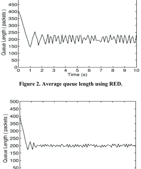
Queue length, link utilization and data dropping be-tween RED-AQM and PSMC-AQM are compared. Fig-ure 2 and FigFig-ure 3 demonstrate that the PSMC-AQM controller considers not only the queue length but also the matching condition of the assemble rate and the link capacity, so it reflects the network condition better than RED. Both of the algorithms can control the queue length near the desired 200 packets, and PSMC-AQM get less data loss rate, so it makes higher link utilization rate. The results are showed in Table 1.
[image:4.595.312.535.94.153.2]
Figure 2. Average queue length using RED.
[image:4.595.59.285.398.530.2]Figure 3. Average queue length using PSMC.
Table 1. Comparison between RED and PSMC.
performance RED PSMC
rate of link
utilization 99.67 99.86
rate of data loss 2.35 0.09
4. Design of Terminal Sliding Mode Control
Algorithm
Last section introduces sliding mode control into the optimization based internet congestion control model, and designs a linear sliding surface, and then validates the effectiveness of the algorithm in simulation. But the sliding mode along the sliding surface is asymptotically stable, that means the converging time could be quite long. For speediness is so important for a router algo-rithm, a special nonlinear sliding surface named terminal sliding surface is proposed in this section. The terminal sliding surface guarantees the finite reaching time to the sliding surface from initial states and the finite reaching time to the origin point. So the converging time is limited, and the speed of the sliding mode control system is en-hanced, further the congestion control performance is improved.
4.1. Design of Terminal Sliding Surface
We design a nonlinear terminal sliding surface as fol-lows:
/ 1 1 2 2 3 1
( ) ( ) ( ) ( ( ))q p
S t d x t d x t d x t , (21)
where >0, >0, >0, p and q are odd positive integers and they satisfy q<p<2q. The sliding surface S(t) corresponds to a combination of the queue length error, the error between incoming traffic rate and link capacity.
1
d d2 d3
When the system state trajectories are on the terminal sliding surface, S(t) satisfies S(t) = 0. So we can obtain the following equality
1 /
2( ) 2 [ 1 1( ) 3( ( )) ]1
q p
x t d d x t d x t . (22)
Substituting (22) into (5), we can obtain the sliding mode dynamics as follows:
1 1
1( ) 2 1 1( ) 2 3( ( ))1
q p
x t d d x t d d x t / . (23)
In order to prove that (23) can converge to the equilib-rium point in finite time, we introduce a lemma as fol-lows
Lemma 1 [13]: Assume that a continuous, positive definite function V (t) satisfies the following differential inequality
( ) ( )
[image:4.595.58.285.406.679.2]where 0, 0 1are constants. Then V(t) satis-fies the following inequality:
1 ( ) 1 (0) (1 )
V t V t, 0 (25)
r
t t
and
( ) 0
V t , t tr (26)
with tr given by
1 (0) (1 ) r V t
. (27)
Theorem 3: The sliding mode dynamics (23) can con-verge to the equilibrium point after the time and satisfies
r
t tr
2(1 ) 1 1 (0) 2 (1 r x t )
, (28)
where x1(0) is the initial value of x t1( ) and
,
1 2 3
d d 2
/ 1
2
q p
.
Proof: Choose a Lyapunov function candidate for the system (23) as follows:
T 1 1
1
( ) ( ) ( ) 2
V t x t x t (29)
then the time derivative of V (t) along (23) is
T 1 1
T 1 1
1 2 1 1 2 3 1
2 /
1 1
2 1 1 2 3 1 / 1 1
2 3 1
( ) ( ) ( ) ( )[ ( ) ( ( )) ] ( ) ( ) ( ) . q p q p q p
V t x t x t
x t d d x t d d x t
d d x t d d x t
d d x t
/
1 (30)
By (29), we have
1( ) 2 ( )
x t V t (31)
Substituting (31) into (30), we can obtain the follow-ing inequality
( ) ( )
V t V t (32)
where 1 ,
2 3
2d d
/ 1
2
q p
.
According to Lemma 1, we know that the sliding mode dynamics (23) can converge to the equilibrium point after the time and satisfies the following
equality tr tr
2(1 ) 1 1 1 (0) (0)
(1 ) 2 (1 )
r x V t
(33)
So the system motion on the terminal sliding surface (21) can converge to the equilibrium point in finite time.
4.2. Design of Terminal Sliding Mode Controller
In the subsection, we design a robust terminal sliding mode controller to satisfy the reaching condition. We consider the following control structure of the form
( ) eq( ) N( )
p t p t p t . (34)
Theorem 4: If the control law is used for system (5) and (6) as follows:
/ 1 1 2 3 1 2 2
2 2 / 1 3 1 1 2 2 ( / ) ( ) ( ) ( ( ) ) , ( ) ( ) ( ) q p eq q p
d x q p d x x d k
p t
d k x C
qd x
d r t C
d kr t pd kr t r t
(35) 2 2 2
( ) sgn( ( ))
( ) .
( )
v N
k S t S S t p t
d k x C
(36)
then the controller can satisfy the reaching condition
2
( ) sgn( ( )) ( )
S t S S t kS t . (37) Proof : Recall (21), the time derivative of S(t) along the trajectory of (5) and (6) under the control (34) is given as
/ 1 1 1 2 2 3 1 1 1 2 2 2
/ 1
3 1 2
( ) ( ) ( ) ( / )( ( )) ( )
( ) ( ( ( ) )) ( ))
( / )( ( )) ( ).
q p
q p
S t d x t d x t d q p x t x t d x t d k x t C p t
d q p x t x t
(38)
Substitute (34) into (38), we can get
2
( ) v ( ) sgn( ( )) S t k S t S S t .
So the controller (34) can satisfy the reaching condi-tion (37). That is to say, the controller can force system state trajectories toward the terminal sliding surface infi-nite time and maintain them on the sliding surface after then. Meanwhile, the reaching rate is fast and chattering is low.
4.3. Simulation Results
In this section the effectiveness and performance of the terminal sliding mode controller (TSMC) is validated by simulations. Common sliding mode controller (SMVS, Sliding Mode Variable Structure) is also simulated for the purpose of comparison with suggested parameter values 0.96, 0.96, given in [15]. We consider the same dumbbell network topology with a single bottleneck link as Figure 1.
The network parameters are chosen the same as Part C of Section 3: the maximum buffer of each router is 500 packets and the link capacity is . The desired queue length d is 200 packets. The initial queue length is 400 packets. And the parameters of TSMC-AQM controller are chosen as 1 , 2
1250packets/s C
1 d d q
1
,
3 1000, , , ,
d q3 p5 k5 0.1. From Theorem 3 we can calculate r 0.5506s.
The simulation is operated under variable network conditions. The link capacity C and the roundtrip time R are varied through the process. Figure 4 and Figure 5 show that the two controllers are insensitive to different TCP loads and link capacity, but TSMC has shorter regulating time and better steady performance than SMVS controller.
t
5. Conclusions
[image:6.595.64.281.348.515.2]In this paper, we combine the Kelly’s optimization scheme and the sliding mode control algorithm to ana-lyze the convergence of the queue. We design two slid-
[image:6.595.64.278.349.693.2]Figure 4. The comparison with variable C.
Figure 5. The comparison with variableR.
ing mode algorithm: the linear and the terminal ones. The simulation results show that both of the algorithms can converge to the equilibrium point in finite time. Ob-viously, the terminal sliding mode control can obtain faster transients and less oscillatory responses under dy-namic network conditions, which translates into higher link utilization, low packet loss rate and small queue fluctuations. And the proposed controller has better sta-bility and robustness than common sliding mode con-troller, which would be meaningful for the congestion control of the Internet.
6. References
[1] B. Braden and D. Clark, “Recommendations on queue management and congestion avoidance in the Internet,” RFC 2309, 1998.
[2] S. Floyd and V. Jacobson, “Random early detection gate-ways for congestion avoidance,” IEEE/ACM Transaction on Networking, Vol. 1, pp. 397-413, 1993.
[3] W. C. Feng, Kang G. Shin, D. D. Kandlur, et al., “The blue active queue management algorithms,” IEEE/ACM Transactions on Networking, Vol. 10, No. 4, pp. 513-528, 2002.
[4] S. Athuraliya, S. H. Low, V. H. Li, et al., “REM: Active queue management,” IEEE Network, Vol. 15, No. 3, pp. 48-53,2001.
[5] S. Srisankar, Kunniyur, and R. Srikant, “An adaptive virtual queue (AVQ) algorithm for active queue man-agement,” IEEE/ACM Transactions on Networking,Vol. 12, No. 2, pp. 266-289, 2004.
[6] C. V. Hollot, V. Misra, D. Towsley, and W. Gong, “On designing improved controllers for AQM routers sup-porting TCP flows,” Proceedings of IEEE INFOCOM, Anchorage, Alaska, USA, IEEE Communications Society, pp. 1726-1734, 2001.
[7] H. Lim, K. J. Park, and C. H. Choi, “Virtual rate control algorithm for active queue management in TCP net-works,” IEEE Electronics Letters, Vol. 38, No. 16, pp. 873-874, 2002.
[8] F. Kelly, A. Maulloo, and D. Tan, “Rate control for communication networks: Shadow prices, proportional fairness and stability,” Journal of the Operational Re-search Society, Vol. 49, No. 3, pp. 237–252, March 1998. [9] Y. H. Roh and J. H. Oh, “Robust stabilization of uncer-tain input-delay systems by sliding mode control with delay compensation,” Automatica, Vol. 35, pp. 1861- 1865, 1999.
[11] P. Yan, Y. Gao, and H. AOzbay, “A variable structure control approach to active queue management for TCP with ECN,” IEEE Transactions on Control Systems Technology, Vol. 13, pp. 203-215, 2005.
[12] F. J. Yin, G. M. Dimirovski, and Y. W. Jing, “Robust stabilization of uncertain input delay for Internet conges-tion control,” Proceedings of the American Control Con-ference, Minneapolis, Minnesota, USA, pp. 5576-5580, 2006.
[13] Y. Tang, “Terminal sliding mode control for rigid ro-bots,” Automatica, Vol. 34, pp. 51-56, 1997.
[14] S. H. Yu, X. H. Yu, B. Shirinzadeh, and Z. H. Man, “Continuous finite-time control for robotic manipulators with terminal sliding mode,” Automatica, Vol. 41, pp. 1957-1964, 2005.
[15] F. Paganini, Z. Wang, J. C. Doyle, and S. H. Low, “Con-gestion control for high performance, stability, and fair-ness in general networks,” IEEE/ACM Transaction on Networking, Vol. 13, No. 1, pp. 43–56, 2005.