Limits on Computationally Efficient VCG Based Mechanisms for Combinatorial Auctions and Public Projects

(1)

Limits on Computationally Efficient VCG-Based

Mechanisms for Combinatorial Auctions and Public Projects

Thesis by

David Buchfuhrer

In Partial Fulfillment of the Requirements for the Degree of

Doctor of Philosophy

California Institute of Technology Pasadena, California

2011

(2)

c

2011

(3)

Acknowledgements

Thanks to Chris Umans for help and advice in researching and writing up everything in this dis-sertation. Thanks to Yaron Singer and Michael Schapira for developing the ideas behind showing computational hardness of VCG mechanisms and for working with me on applying these ideas to pub-lic projects. Thanks to Shaddin Dughmi for helping me work through different possible approaches to the material in Chapter 5. Thanks to John Ledyard for giving me an economist’s perspective on the problems I was studying and helping me evaluate and eliminate several approaches to eliminating the asymmetry described in Chapter 5. Thanks to my committee members John Ledyard, Leonard Schulman, Chris Umans, and Adam Wierman for taking the time to evaluate my thesis proposal and provide helpful comments.

(4)

Abstract

A natural goal in designing mechanisms for auctions and public projects is to maximize the social welfare while incentivizing players to bid truthfully. If these are the only concerns, the problem is easily solved by use of the VCG mechanism. Unfortunately, this mechanism is not computationally efficient in general and there are currently no other general methods for designing truthful mech-anisms. However, it is possible to design computationally efficient VCG-based mechanisms which approximately maximize the social welfare.

We explore the design space of computationally efficient VCG-based mechanisms under submod-ular valuations and show that the achievable approximation guarantees are poor, even compared to efficient non-truthful algorithms. Some of these approximation hardness results stem from an asymmetry in the information available to the players versus that available to the mechanism. We develop an alternativeInstance Oracle model which reduces this asymmetry by allowing the mecha-nism to access some computational capabilities of the players. By building assumptions about player computation into the model, a more realistic study of mechanism design can be undertaken.

(5)

Introduction

Combinatorial auctions and combinatorial public projects are two important allocation problems in algorithmic mechanism design. The goal of each is to find a suitable allocation. A combinatorial auction consists of a set of m items and n players. An allocation in a combinatorial auction is a partition of the items S1, . . . , Sn such that each player gets the setSi ⊆[m], and Si∩Sj =∅ for

i 6=j. Some items may not be given to any player. A combinatorial public project consists of m

items, n players, and a parameter k. An allocation in a combinatorial public project is a subset

S⊆[m] of the items of size|S|=k.

In both cases, each player i has a value function vi over subsets of the items. Each value

function is assumed to be non-negative (vi(S) ≥ 0), non-decreasing (vi(S) ≥ vi(T) for S ⊇ T),

and normalized (vi(∅) = 0). We also assume that players only care about their own value, and not

about the value obtained by others. A mechanism for either of these problems takes in the valuation functions v1, . . . , vm and returns an allocationA and a list of pricesp1, . . . pn, where playeri must

pay pricepi. Being rational, each player seeks to maximize his quasi-linear utility functionvi(A)−pi

(vi(Si)−pi for combinatorial auctions orvi(S)−pi for combinatorial public projects).

Before studying this problem, it is important to determine the goal which we wish the mechanism to achieve. One natural goal is to maximize the revenue,P

ipi. Revenue maximization is important

and well-studied [31, 39, 40, 9, 26, 27, 11], but is not the goal we consider. Instead, we look at maximization of thesocial welfare,P

ivi(A).

From a purely computational perspective, the complexity of this problem depends only on how hard it is to find an allocation A maximizing or approximating the maximum value of P

ivi(A).

(8)

result in negative utility) and no player benefits by declaring a lower price (as this does not decrease the payment for the player declaring a lower price). As everyone benefits most from declaring their valuation correctly, we can assume that rational players will make truthful declarations under this mechanism. Therefore, this mechanism results in the player with highest value getting the item.

The second-price mechanism for single item auctions was famously generalized by the Vickrey-Clarke-Groves (VCG) mechanism [42, 10, 25]. In this rather simple scheme, one simply calculates an optimal allocation A, then for each player i, calculate an optimal allocationA−i for all players

excluding i. Player i is then charged price pi = P_j₆₌_ivj(A−i)−vj(A) equal to the decrease in

social welfare of other players due toi’s participation. Playeriis therefore incentivized to maximize

vi(A) +Pj6=ivj(A)−Pj6=ivj(A−i), which is the social welfare, minus a term that does not depend

on what player i declares. Thus, each player is incentivized to maximize the social welfare. So a truthful mechanism is always available for maximizing welfare.

Further demonstrating the importance of the VCG mechanism, Roberts showed that for suf-ficiently general problems, the VCG mechanism is the only truthful mechanism [38]. More recent work has also made progress on demonstrating this result for more restricted problems [2, 29, 18, 36]. So the VCG mechanism is not only important because it is a truthful mechanism. It is important because in many cases, it is the only truthful mechanism.

This can be problematic from a computational perspective. When finding an optimal allocation is computationally infeasible, the VCG mechanism cannot be implemented. One might be tempted to implement the VCG mechanism using an approximation algorithm, but the VCG mechanism is only truthful ifP

ivi(A) is always maximized by truthful reporting of valuation functions. [34]

described the class of approximation algorithms which can be truthfully implemented using the VCG mechanism, which are known asmaximal-in-range algorithms.

Every algorithm has a range R of possible allocations it can output depending on the input given. For many familiar algorithms, R will be the set of all possible allocations. A maximal-in-range algorithm always outputs an allocation A = argmax_A_∈_RP

ivi(A) which maximizes social

welfare within the range. Maximal-in-range algorithms can be tricky to design, as it can be difficult to find a range which contains a good approximation of the social welfare for any instance and for which the welfare-maximizing allocation can be efficiently found. The restriction to maximal-in-range mechanisms can dramatically worsen the best achievable approximation ratio [14, 36].

1.1 Definitions and Notation

(9)

functions. Valuation functions are central to the problems studied in this dissertation, as they define the preferences of the players.

Definition 1.1(Valuation Function). A valuation functionvis a functionv: 2[m]→R+∪ {0}from

subsets of[m] ={1, . . . , m}to the non-negative real numbers. A valuation function is normalized to

v(∅) = 0 and monotone, so thatv(S∪T)≥v(S) for all setsS, T.

In order to achieve the best possible outcome, we wish to maximize the the overall sum of player valuations. We call this sum the social welfare.

Definition 1.2 (Social Welfare). The social welfare of an allocation is the sum over each player of the player’s value for the allocation. If there are n players with valuation functions v1, . . . , vn,

the social welfare ofA isP

ivi(A). The social welfare of a combinatorial auction or combinatorial

public project is the maximum social welfare of any allocation,maxAPivi(A).

The first problem we consider is the combinatorial public project problem.

Definition 1.3(Combinatorial Public Project). A combinatorial public project consists ofnplayers [n], m items [m], and a parameter k. Each player i has a valuation function vi. An allocation A

consists a subset S of [m]of size k. The social welfare of AisP

ivi(S).

We also study combinatorial auctions.

Definition 1.4 (Combinatorial Auction). A combinatorial auction consists ofnplayers[n] andm

items[m]. Each playeri has a valuation functionvi. An allocation A consists ofn subsets of[m],

S1, . . . , Sn such thatSi∩Sj =∅ fori6=j. The social welfare of AisPivi(Si).

All valuations which we study are subadditive.

Definition 1.5 (Subadditive). A valuation functionv is subadditive ifv(S∪T)≤v(S) +v(T)for all sets S, T.

Most of the functions we study are also submodular.

Definition 1.6 (Submodular). A valuation function v is submodular if v(S∪T) +v(S∩T) ≤ v(S) +v(T)for all sets S, T.

In both auctions and public projects, players wish to maximize their utility.

Definition 1.7 (Utility). Given a valuation functionv and a set of pricesp1, . . . , pm, the utility of

a setS isv(S)−P

i∈Spi.

A set which maximizes utility is called a demand set.

Definition 1.8(Demand Set). Given a valuation functionvand a set of pricesp1, . . . , pm, a demand

set is a set S maximizing the utility,v(S)−P

(10)

Demand sets are not important just because of their relation to utility maximization. They are also necessary to define the class of gross substitutes, which contains several of the valuation classes we study.

Definition 1.9 (Gross Substitutes). A valuation function v satisfies the gross substitutes property if for any two sets of pricesp1, . . . , pm and q1, . . . , qm such thatqi≥pi andS is a demand set for

p1, . . . , pm, that there exists some demand set T forq1, . . . , qm such thatS∩ {i:pi =qi} ⊆T. In

other words, the items which were already demanded and did not have their prices raised remain in a demand set.

We call the process that leads to allocations and prices a mechanism.

Definition 1.10 (Mechanism). A mechanism M is an algorithm which takes in an instance of an allocation problem and returns an allocationA and a list of pricesp1, . . . , pn.

The mechanisms that we are interested in are those in which players are not incentivized to lie about their valuations. These are called truthful mechanisms.

Definition 1.11 (Truthful Mechanism). A mechanism M is truthful if for any player with value

vi and any values v1, . . . , vi−1, vi+1, . . . , vn for players other than i, player i’s utility vi(A)−pi is

maximized by declaringvi.

One way to create a maximal-in-range mechanism is through the use of VCG payments.

Definition 1.12(VCG Payments). The VCG payment for playerigiven an allocation algorithmA

is defined as follows. Let S be the allocation determined byi given all player values, andS−i be the

allocation Adetermines if we replace vi with 0. The VCG payment ispi=Pj6=ivj(Si)−vj(S−i).

VCG payments result in a truthful mechanism if the algorithm they are applied to is maximal-in-range.

Definition 1.13 (Maximal-in-Range (MIR)). An allocation algorithm A is maximal-in-range if there exists a set of values CS for each set S such that for any valuation functions v1, . . . , vn, A

returns a set S which maximizes P

ivi(S)over the range ofA.

The use of a maximal-in-range algorithm together with VCG payments is the only known general way to truthfully maximize social welfare, and remains an active area of study [16, 18, 29, 36]. We call mechanisms which use maximal-in-range algorithms with VCG payments VCG-based mechanisms. Maximal-in-range algorithms are a special case of affine maximizers.

Definition 1.14 (Affine maximizer). An allocation algorithm A is an affine maximizer if there exists a set of valuesCS for each setS such that for any valuation functionsv1, . . . , vn,Areturns a

setS which maximizesP

ivi(S) +CS over the range ofA. Note that maximal-in-range mechanisms

(11)

1.1.1 Notation

A class of combinatorial auction or combinatorial public project problem can be defined by three important factors. The first is the type of problem, auction, or public project. The second is the class of valuation functions that v1, . . . , vn belong to. Finally, we have the number of players

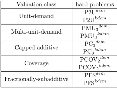
n. Individual problems will also have different numbers of items m and for combinatorial public projects, parameters k. But we classify instances by type of problem, class of valuation functions, and number of players. All three of these factors can affect the difficulty of mechanism design. In order to clearly express what each of these factors are, we use a three-part notation. We will explain this notation using the exampleP C2, which we will now explain.

The first part of the notation denotes whether the problem is a combinatorial auction or a combinatorial public project. For a combinatorial auction, we use an A and for a combinatorial public project, we use aP. So in the exampleP C2, the problem is a combinatorial public project.

The second part denotes the class of valuation functions allowed. This is simply one or more letters following theAorP. In the exampleP C2, the class of valuation functions is the one denoted byC, which refers to capped-additive valuations. We will define capped additive valuations as well as other valuation classes and how they are denoted in Section 1.1.2.

The final part of the notation is an optional subscript. If present, it is the number of players. If not, the number of players is not limited. SoP C2is the combinatorial public projects problem with 2 capped-additive players andP C is the combinatorial public projects problem with an unbounded number of capped-additive players.

1.1.2 Problem Definitions

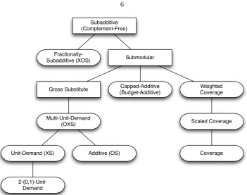
In this dissertation, we study problems for which the valuation functions are subadditive. This class of functions (also known as complement-free) is important to the study of combinatorial auctions [15, 22, 23, 30, 44]. In particular, we study valuation functions drawn from a complement-free hierarchy (see Figure 1.1) based on the classes studied in [30, 33]. The classes we study in this hierarchy are defined below. All of the submodular valuation functions havesuccinct representations.

Definition 1.15(Succinct Representation). A valuation class has a succinct representation if func-tions in the class can be uniquely identified by a representation which has size polynomial in the number of itemsmand in log(vi([m])), the log of the maximum value for any set.

(12)

Subadditive (Complement-Free)

Fractionally-Subadditive (XOS) Submodular

Gross Substitute _{(Budget-Additive)}Capped-Additive Weighted _Coverage

Multi-Unit-Demand (OXS)

Unit-Demand (XS) Additive (OS)

Scaled Coverage

Coverage

[image:12.595.150.502.53.330.2]

2-{0,1}-Unit-Demand

Figure 1.1: The Complement-Free Hierarchy. The valuation classes studied directly in this dis-sertation are marked by rounded nodes. The names in parentheses are alternative names which are sometimes also used to refer to these classes. We do not use these alternative names in this dissertation.

Definition 1.16(Additive (A)). An additive valuationvihas valuevji for each itemj and the value

of a set S is vi(S) =P_j_∈_Svij. Additive valuations are not discussed much in this dissertation, as

we can show fairly easily that both PA and AA have polynomial-time solutions (see Theorem 1.2). Before proving that PA and AA have polynomial-time solutions via Theorem 1.2, we require a helpful lemma.

Lemma 1.1. There exists an algorithm which for any k, m, finds the k largest or smallest items from an unordered array of length minO(m)time.

Proof. We will show how to find thek largest items. To find the k smallest items, simply reverse the comparisons in this process. [3] shows that thekth largest item in an array of lengthmcan be found inO(m) time independent of k. To find the otherk−1 larger items, simply iterate through the array twice. On the first pass, add any items which are greater than thekth largest item to the list of the kth largest items. This pass may result in a list of length less than k, as there may be some items equal to thekth largest which belong on the list. So on the second pass, add items equal to thekth largest item until the list hask items.

(13)

or equal to thekth largest item (including itself). Therefore, this list contains the klargest items. Since finding the kth largest item takes O(m) time, as do each of the 2 passes, the total running time of this algorithm isO(m).

Theorem 1.2. Both AA and PA can be solved in O(mn)time wheremis the number of items and

nis the number of players.

Proof. For AA, the social welfare is simplyP_vj

i over pairsi, jsuch that itemjis assigned to player

i. So this is maximized by assigning each itemj to the playeriwith the maximum value ofvj_i. For each item it only takesO(n) time to find this maximum, for a total ofO(mn) time overmitems.

For PA, the social welfare of a set S isP

j∈S

P

iv j

i. So to maximize the social welfare, simply

choose thekitems with highest value forP

iv j

i. Thesemsums can be found inO(n) time each, for

a total ofO(mn) time. By Lemma 1.1, thek highest sums can then be found in O(m) time, for a total ofO(mn) time.

Definition 1.17 (Unit-Demand (U)). A unit-demand valuation vi has a value vij for each item j

and the value of a set S is the maximum value of any item in S, vi(S) = maxj∈Svji. vi can be

succinctly represented by the mvalues vj_i.

Definition 1.18 (`-{0,1}-Unit-Demand (`U)). An `-{0,1}-unit-demand valuation vi is a

unit-demand valuation for which vij is either 0 or 1 for each j, and for which v j

i = 1 for at most `

values ofj.

We will mostly consider the 2-{0,1}-unit-demand valuation (2U).

Definition 1.19(Multi-Unit-Demand (MU)). A multi-unit-demand valuationviconsists of several

unit-demand valuations v(ij). In order to compute the valuevi(S) of a set S, one item is assigned

to each unit-demand valuation function, and the values for each function are summed. The value is the maximum possible such sum,

vi(S) = max S1,...,S`

Si⊆S Si∩Sj=∅

X

j

vi(j)(Sj).

Lemma 1.3 shows thatvi(S)is computable in polynomial time. Lemma 1.5 shows that any

multi-unit-demand function vi can be succinctly represented by at most m2 unit-demand valuation functions.

Lemma 1.3. Ifviis a multi-unit-demand valuation function overmitems, it is possible to compute

vi(S) = max S1,...,S`

Si⊆S Si∩Sj=∅

`

X

j=1

vi(j)(Sj)

(14)

Proof. Given a partition S1, . . . , S` of S, the value computed by the partition is P`j=1v (j)

i (Sj) =

P`

j=1v (j)

i ({s∗j}) for somes∗j in eachSj. So in order to maximize the value, we need only to optimally

match each valuation function to an item. This can be accomplished via maximum weighted bipartite matching. Create a bipartite graph in which one side has m nodes corresponding to the items, and the other has ` nodes corresponding to the functions v(1)i , . . . , v

(`)

i . The edge between nodes

corresponding to itemj and functionv(ij)has weightv

(j0₎

i (j). Thus, a maximum weighted matching

maximizes P

vi(j0)(j) over all matchings of items j to functions v

(j0₎

i . As a maximum weighted

matching on a bipartite graph with m+` nodes can be found in time polynomial in mand`, this completes the proof.

Computing the value of a setS for a single multi-unit-demand player is equivalent to computing an optimal allocation in an auction with several such players. So Lemma 1.3 implies the following corollary.

Corollary 1.4. AMU (and therefore also AU) can be solved exactly in polynomial time.

Proof. Suppose we have n players with multi-unit-demand functions v1, . . . , vn, where vi(S) =

maxS1,...,S`i

P

jv

(j)

i (Sj). We create a single multi-unit-demand function V with unit-demand

func-tionsV(i,j)₌_v(j)

i . The value of a setS is the maximum over all partitions

S(1,1), . . . , S(1,m), S(2,1), . . . , S(2,m), . . . , S(n,1), . . . , S(n,m)

ofP

(i,j)v (j)

i (S(i,j)). Note that this is equivalent to giving playeriSjS(i,j). So the maximum social welfare in the AMU instance is the value of [m] to the single player we have created. Therefore, Lemma 1.3 shows that AMU can be solved exactly in polynomial time.

Lemma 1.5. For any multi-unit-demand valuationvi(S) =P`_j₌₁vi(j)(S), there is a set M of size

at mostm2 _{such that}

vi(S) = max S1,...,S`

Si⊆S Si∩Sj=∅

X

j∈M

v(ij)(Sj).

Furthermore, this set can be found in O(m`)time. Proof. If`≤m, this is trivially true. So assume` > m.

(15)

Lemma 1.1 shows that we can find the m functions of highest value for item j in O(`) time. Since this is repeatedmtimes, once for each item, the total time is O(m`).

Definition 1.20 (Capped-Additive (C)). A capped-additive valuationvi has valuevji for each item

j and a value capc. The value of a setS is the minimum of the sum of all values inS and the value cap,vi(S) = min(Pj∈Sv

j

i, c). vi can be represented succinctly by them valuesvij=vi({j})and the

budget capci=vi([m]).

Definition 1.21(Coverage (COV)). A coverage valuationvi has a subsetVij⊆U of some universe

U associated with each itemj and the value of a setS is the size of the union of the corresponding sets, vi(S) =

S

j∈SV j i

. vi can be represented succinctly by the sets V

j

i if |U| has a polynomial

bound.

Definition 1.22 (Scaled Coverage Valuation (SCOV)). A scaled coverage valuationvi has a subset

V_ij ⊆U of some universeU associated with each itemj as well as a scaling factor αand the value of a setS isαtimes the size of the union of the corresponding sets,vi(S) =α

S

j∈SV j i

. vi can be

represented succinctly by the sets V_ij together with the scale factorαif|U| has a polynomial bound.

Definition 1.23 (Weighted Coverage Valuation (WCOV)). A weighted coverage valuationvi has a

subsetV_ij ⊆U of some universeU associated with each itemjas well as a weightwufor eachu∈U.

The value of a setS is the size of the sum ofwu over items ucovered by sets Vij corresponding to

itemsj∈S,

vi(S) =

X

u∈S

j∈S Vj

i

wu.

vi can be represented succinctly by the setsVij together with the weightswu if |U|has a polynomial

bound.

Definition 1.24(Fractionally-Subadditive (FS)). A fractionally-subadditive valuationvihas`

addi-tive functionsv_i(1), . . . , v_i(`). The value of a setSis the maximum value over the`additive functions,

vi(S) = maxjv(ij)(S). vi is represented by the` additive functions v(1)i , . . . , v

(`)

i . Lemma 1.6 shows

that arbitrary vi cannot be represented succinctly regardless of choice of representation. As we are

interested in valuations with succinct representations, our results deal with`∈poly(m), making our representations succinct.

Lemma 1.6. For eachm >0and any choice of representation, there exists a fractionally-subadditive valuation function vi for2mitems with vi(S)≤2m2 which requires at least2mbits to represent.

Proof. We will prove this by showing that there are at least 2(2mm) fractionally-subadditive valuation functions. As there are only 2(2mm)−_{1 strings with fewer than} 2m

m

bits, this proves that 2_mm

bits are required for at least one of these valuations. The binomial coefficient 2_mm

(16)

number of subsets of [2m] of size m and 2m is the number of subsets of [m]. For each subset M

of [m], there is a corresponding subset M0 _{of [2}_m_{] of size} _m _{containing all elements of} _M_{, plus}

items m+ 1, . . . , m+ (m− |M|). Thus, 2_mm

≥ 2m, so showing that there are 2(2mm) different fractionally-subadditive functions overmitems proves that one of them requires at least 2mbits to represent.

The 2(2mm) valuation functions are defined as follows. Let [2m] m

be the set of subsets of [2m] of sizem. For each M ⊆ [2_mm]

, let

vM(S) =

 



(m+ 1)· |S|, |S|< morS ∈ M m· |S|, |S| ≥mandS /∈ M .

LetM,M0 _{be distinct subsets of} [2m]

m

. We will show thatvMandvM0 are different functions. As

MandM0 _{are different, there exists some set}_S _{that is in one of them but not the other. Without}

loss of generality, assume M contains some set S that M0 _{does not. By the above definition,}

vM(S) = (m+ 1)·m, as all sets inMhave sizem. AsS /∈ M0,vM0(S) =m·m, which is different from (m+ 1)·mform >0. ThusvM6=vM0 for everyM 6=M0, so there are 2(

2m

m) distinct functions

vM, one for each setM ⊆ [2_mm].

To complete the proof, we need only see that for everyM ⊆ [2_mm]

,vMis fractionally-subadditive.

We construct additive functionsvT

M for eachT ⊆[2m] as follows. For|T|< mor T ∈ M,

vMT ({s}) =

 



m+ 1, s∈T

0, otherwise

.

For|T| ≥mandT /∈ M,

vMT ({s}) =

 



m, s∈T

0, otherwise

.

This defines the additive functionsvT

M(S) =

P

s∈SvMT ({s}). Using these, we define the

fractionally-subadditive function

vM(S) = max

T v T

M(S).

For anyT,vT

M(S)≤(m+1)·|S|. If|S|< morS∈ M,vSM(S) = (m+1)·|S|. SovM(S) = (m+1)·|S|.

ForS > m, we consider two cases. For|T| ≤m,vT

M(S)≤m·(m+ 1), as eachs∈T has value at

mostm+ 1 and|T| ≤m. Since|S|> m, this is at mostm· |S|. For|T|> m, the value of each item is at mostmand there are only|S|items, for a total value of at most|S| ·m. SincevS

M(S) =m· |S|

achieves this bound,vM(S) =m· |S|.

(17)

m−1 items in bothS and T, so the maximum value is again at most (m+ 1)·(m−1)< m· |S|. For|T| ≥m, T /∈ M, the value is at mostm· |S|, which is achieved byvS

M(S). So vM(S) =m· |S|.

By the above three cases, we have shown that

vM(S) =

 



(m+ 1)· |S|, |S|< mor S∈ M m· |S|, |S| ≥mandS /∈ M

is fractionally-subadditive, completing the proof.

1.2 Overview of Results

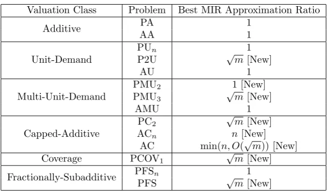
In Chapters 3 and 4 we show hardness results for VCG-based mechanisms for combinatorial public projects and combinatorial auctions, respectively. These results for the valuation classes studied in this dissertation are summarized in Figure 1.2.

Valuation Class Problem Best MIR Approximation Ratio

Additive PA 1

AA 1

Unit-Demand

PUn 1

P2U √m[New]

AU 1

Multi-Unit-Demand

PMU2 1 [New]

PMU3 √m[New]

AMU 1

Capped-Additive

PC2

√

m[New]

ACn n[New]

AC min(n, O(√m)) [New]

Coverage PCOV1 √m[New]

Fractionally-Subadditive PFSn 1

[image:17.595.164.484.311.498.2]

PFS √m[New]

Figure 1.2: The best approximation ratios achievable by a polynomial-time maximal-in-range algo-rithm assuming that NP does not have polynomial circuits. Whennis used as a subscript, it refers to any constantn. A√mupper bound for public projects with subadditive players is shown in [41], so all√mare proven in this dissertation via a lower-bound ofm1/2− _{for all}_>_0.

For certain cases in Chapter 3, we are able to show a few results about general truthful mech-anisms. VCG-based approximation algorithms cannot approximate P2U with a ratio better than

√

m, but we show a truthful 2-approximation. We extend the VCG-based hardness result for PCOV1 to show that any polynomial-time truthful mechanism for PSCOV1 cannot approximate the social welfare better than√m unless NP has polynomial circuits.

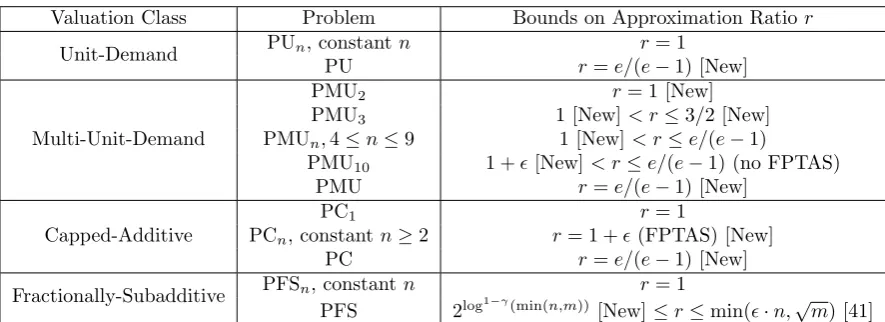
In Chapter 3, we also show some computational results which do not take truthfulness into account. These results are summarized in Figure 1.3.

(18)

Valuation Class Problem Bounds on Approximation Ratior

Unit-Demand PUn, constantn r= 1

PU r=e/(e−1) [New]

Multi-Unit-Demand

PMU2 r= 1 [New]

PMU3 1 [New]< r≤3/2 [New] PMUn,4≤n≤9 1 [New]< r≤e/(e−1)

PMU10 1 +[New]< r≤e/(e−1) (no FPTAS)

PMU r=e/(e−1) [New]

Capped-Additive

PC1 r= 1

PCn, constantn≥2 r= 1 +(FPTAS) [New]

PC r=e/(e−1) [New]

Fractionally-Subadditive PFSn, constant n r= 1 PFS 2log1−γ

[image:18.595.104.547.70.231.2]

(min(n,m)) _[New]_≤_r_≤_min(_·_n,√_m_{) [41]} Figure 1.3: Computational results shown in Chapter 3. Equality refers to matching upper and lower bounds, up to arbitrarily smallfactors. Alle/(e−1) upper bounds are from [32]. Whenis used, it refers to any constant >0.

(19)

Chapter 2

Alternate Approaches

In this chapter, we consider approaches to the study of truthful mechanisms which are not the focus of this dissertation. These approaches are randomized algorithms and communication complex-ity. Outside of this chapter, our primary interest is the computational complexity of deterministic algorithms.

2.1 Randomized Algorithms

Our hardness results only hold for deterministic mechanisms. Recent results [13, 19, 20] show that randomization can sometimes allow for improved approximation ratios. In particular, [19] shows that there exists a randomized FPTAS for ACn for any constant n which satisfies a randomized

notion of truthfulness. Other results have shown that randomization can be of no help depending on the problem and the version of randomized truthfulness used [7, 12].

A universally truthful mechanism is one which chooses a truthful mechanism from some distri-bution, then runs it. Universally truthful mechanisms can also be used to improve on the hardness results for PU, PMU, and PC, as we show in Theorem 2.1 and Corollaries 2.3, 2.4, and 2.5 below.

Definition 2.1 (Universally Truthful). A universally truthful mechanism M consists of several truthful mechanisms M1, . . . , M`. M chooses a mechanism Mi randomly from some distribution

and runs it in order to determine an allocation and payments.

Theorem 2.1. There exists a universally truthful mechanism for PU which runs in O(km) time and achieves an expected approximation ratio of at mostn/k.

Proof. For each subsetT ⊆[m],|T|=kwe define a mechanismMT. MT arbitrarily orders elements

(20)

and adds items according to

Si=

 



Si−1∪ {argmaxjv j

ti}, argmaxjv j

ti∈/Si−1

Si−1∪ {minj /∈Si−1j}, otherwise

where argmax_jvjti refers to any single item j which maximizesv j

ti. MT sets pi= 0 for all i, so no players make payments. The universally truthful mechanism chooses a sizeksubsetT uniformly at random, and uses mechanismMT.

An item is added at each step, so|Sk|=kand we end up with a valid allocation. To see that this

allocation has an expected social welfare of at leastk/n, first note that players inT have their values maximized by construction. As we are choosingT uniformly at random, each player has chancek/n

to be in the firstT, so each player gets at least ak/nfraction of his maximum value in expectation. Thus, the expected approximation ratio is at mostn/k.

Now, we need only see that eachMT is truthful and runs in polynomial time. Playersi /∈T are

ignored, so they have no incentive to lie. Players inT have their value maximized, so they also have no incentive to lie. Thus,MT is truthful.

MT runs in timeO(km) independent ofT. There arekiterations to compute the setsS1, . . . , Sk.

Each iteration only requires finding argmax_jvijand minj /∈Si−1v

j

i, each of which can be found inO(m)

time. Checking whether argmax_jvij is inSi−1takes O(|Si−1|)⊆O(m) time. Thus, each step takes

O(m) time. vti(Si−1) is then compared to maxjv j

ti, with the corresponding item possibly being added toSi−1 to arrive at Si. As there are only m such values, this step also only requiresO(m)

time. So each iteration requires onlyO(m) time, for a total ofO(km) time.

The idea in Theorem 2.1 can be generalized to show that for any valuation functionV and any constant `, that if PV` can be solved exactly, there is a universally truthfuln/`approximation for

PV.

Theorem 2.2. Let V be a class of valuation functions. If PV` can be solved exactly in polynomial

time, there exists a polynomial time universally truthful mechanism which approximates the social welfare of PV with a ratio ofn/`.

Proof. Similarly to the proof of Theorem 2.1, we construct a mechanismMT for each subset T ⊆

[n],|T|=`. This mechanism runs an algorithm which exactly maximizes the social welfare for the players in T and ignores all other players. This is different from the mechanism in the proof of Theorem 2.1 in that we find anS which maximizes P

i∈Tvi(S) rather than maximizing vi(S) for

eachi∈T. Players outside ofT are charged 0 and players inT are charged VCG payments. Let S∗ _{be an optimal allocation and} _A

(21)

welfare is

X

T⊆([n]

`) 1 n ` X

i∈[n]

vi(AT).

As the players in T maximize their social welfare, P

i∈[n]vi(AT)≥Pi∈Tvi(S∗). So the expected

social welfare is at least

X

T∈([n]

`) 1 n ` X

i∈T

vi(S∗) =

1

n `

X

T∈([n]

`)

X

i∈T

vi(S∗).

Since each player i appears in n_`₋−₁1

sets T of size `, the above double summation is equal to

P

i∈[n]

n−1

`−1

vi(S∗). Note that` n_`=n n_`₋−₁1(as both count the number of ways to select a

com-mittee of size`with a chairperson from a group ofnpeople), so 1

n `

=

` n n_`₋−₁1.

Using this identity, we get a total social welfare of at least

1

n `

X

i∈[n]

_n₋₁ `−1

vi(S∗) = n−1

`−1

n `

X

i∈[n]

vi(S∗)

= `

n−1

`−1

n n_`₋−₁1 X

i∈[n]

vi(S∗)

= `

n X

i∈[n]

vi(S∗).

So this mechanism has an expected value of at least`/ntimes the maximum social welfare, giving an expected approximation ratio of at mostn/`.

Now, we need only to see that this is universally truthful and runs in polynomial time. Each

MT is truthful for players outside of T because their valuations do not affect the outcome. MT

runs in polynomial time if PV` can be solved exactly in polynomial time, and truthfulness follows

from the use of VCG payments.

Using Theorem 2.2, we get the following corollaries.

Corollary 2.3. For any constant `, there exists a polynomial-time universally truthful mechanism for PFS which achieves an expected approximation ratio of at mostn/`.

Proof. This follows from Theorem 2.2 and Theorem 3.21, which shows that PFS` can be solved in

polynomial time for any constant`.

(22)

Proof. This follows from Theorem 2.2 and Theorem 3.13, which shows that PMU2can be solved in polynomial time.

Corollary 2.5. There exists a polynomial-time universally truthful mechanism for PC with an expected approximation ratio of at most n.

Proof. This follows from Theorem 2.2. We need only see that PC1 can be solved exactly in poly-nomial time. Clearly, allocating thek items of highest value to the single player will maximize the social welfare. Thus, PC1can be solved in polynomial time, completing the proof.

2.2 Communication Complexity

Another approach to showing the hardness of mechanism design is communication complexity. Rather than show that a problem is difficult to compute the answer to or that truthfulness combined with computational efficiency leads to inapproximability, a communication complexity approach shows that even attaining enough information to solve the problem requires excessive communi-cation. If a problem requires exponential communication to solve, then it is impossible to find a polynomial-time solution regardless of truthfulness. This approach has been useful for demonstrating hardness of subadditive auctions [17, 28, 35] and, more recently, public projects [12].

Unfortunately, this strategy does not work for problems where the valuations have succinct representations. If each valuation functions can be represented in space polynomial in m, then each player need only communicate polynomial information to the mechanism in order for an exact solution to be found, after which VCG payments allow for an exact truthful solution. We restrict our attention in this dissertation to succinctly represented valuations.

Succinct representation need not be a complete barrier to communication complexity results. Query models limit the communication to the mechanism posing certain questions to the players, then receiving the answer back. The two query types of interest in this dissertation are value queries and demand queries.

Definition 2.2(Value Query). A value asks what the value of a setS is to playeri. A value query thus consists of a setS. The response to a value query isvi(S).

Definition 2.3(Demand Query). A demand query asks for a demand set for playeriunder prices

p1, . . . , pm. A demand query thus consists of a set S and a set ofmpricesp1, . . . , pm. The response

to a demand query is a set S maximizing vi(S)−Pj∈Spj.

A polynomial number of demand queries are sufficient to compute a value query [4], so demand queries are strictly more powerful.

(23)

Lemma 2.6. PFS1 requires exponential communication to solve exactly if communication is limited to value queries. Furthermore, this is true even whenv1 is chosen from a set of valuation functions which can be represented inO˜(m2₎_bits.

Proof. We will build a function by first picking a set T ⊆ [m] of size |T| = m/2. We build the fractionally subadditive function out of the following additive functions. Fori= 1, . . . , m,

v₁(i)(S) =

 



1, i∈S

0, otherwise

as well asv(₁m+1)(S) = 2|S|/mand v₁(m+2)(S) = |S∩T|(2/m+ 1/m2_{). Set} _v

1(S) = maxiv1(i)(S).

v1(1), . . . , v (m+2)

1 require Õ(m) bits each, as they each need only have mvalues, 1 for each item, and each value requires Õ(1) bits. As there are O(m) functions each requiring Õ(m) bits, there are a total of Õ(m2_{) bits required to represent}_v_1.

Claim 2.6.1.

v1(S) =

    

   

1, 0<|S|< m/2 1 + 2/m, S=T

2|S|/m, otherwise

.

Proof. First, letS=∅. Thenv1(S) = 0, as all of the functions thatS consists of are additive. This corresponds to the above case 2|S|/m= 2(0)/m= 0.

If 0 < |S| < m/2, v(1i)(S) ∈ {0,1} for i ≤m and for every i ∈ S, v (i)

1 (S) = 1. So v1(S)≥1. Furthermore,

v1(m+1)(S) = 2|S|/m

< 2(m/2)/m

= 1

and

v₁(m+2)(S) = |S∩T|(2/m+ 1/m2₎

≤ |S|(2/m+ 1/m2)

≤ (m/2−1)(2/m+ 1/m2) = 1 + 1/m−(2/m+ 1/m2) = 1−1/m−1/m2

(24)

Sov1(S) = 1.

Now, consider S=T.

v(1m+2)(T) = |T∩T|(2/m+ 1/m2) = |T|(2/m+ 1/m2) = (m/2)(2/m+ 1/m2₎ = 1 + 2/m

v1(i)(T)≤1<1 + 2/mfori≤m, so these won’t be the maximum.

v₁(m+1)(T) = 2|T|

m

= 2(m/2)

m

= 1

< 1 + 2/m,

so this isn’t the maximum either. Sov1(T) = 1 + 2/m.

Now, suppose |S|=m/2, S6=T. AsS 6=T,|S∩T|<|S|=m/2, so|S∩T| ≤m/2−1. So

v₁(m+2)(S) = |S∩T|(2/m+ 1/m2) = (m/2−1)(2/m+ 1/m2)

= m/2(2/m+ 1/m2)−(2/m+ 1/m2) = 1 + 1/m−(2/m+ 1/m2₎

< 1 + 1/m−1/m

= 1

v1(m+1)(S) = 2|S|/m= 1. Fori≤m,v (i)

1 (S)≤1. Sov (m+1)

1 (S) = 1 = 2|S|/m.

Finally, let |S| > m/2. v(₁m+1)(S) = 2|S|/m. As |S| > m/2, 2|S|/m ≥ 1 + 2/m. Note that

|S∩T| ≤ |T|=m/2, so

v(1m+2)(S) = |S∩T|(2/m+ 1/m2)

≤ (m/2)(2/m+ 1/m2) = 1 + 1/(2m)

(25)

Fori≤m,v1(i)(S)≤1<2|S|/m, so the maximum value isv1(S) = 2|S|/m.

Now, consider an instance of PFS1 with a single player whose valuation is constructed as above for someT andk=m/2. For any allocation S=6 T,|S|=m/2, so the social welfare is 2|S|/m= 1. If T is allocated, the social welfare is 1 + 2/m. Thus, in order to maximize the social welfare, T

must be allocated.

We now show that finding T requires exponentially many value queries in the worst case. In particular, we show that this requires _m/m₂

−1 queries. Suppose a query is made with a set

S,|S| 6=m/2. In this case,v1(S) only depends on|S|. So nothing is learned aboutT by making this query. Now, suppose|S|=m/2. Thenv1(S) = 1 regardless ofT ifS6=T and 1 +m/2 ifS=T. So ifS6=T, this query only rules outS.

Suppose we make queries S = {S1, . . . , S`} where Si 6= T for all I, and let T = {S : |S| =

m/2, S /∈ S}. For everyS ∈ T, S =T is consistent with the queries so far. So while|T | >1, we don’t know what T is, so for some T, the next query is not T. Thus, in the worst case, we make queries S 6= T until |T | = 1. As |T | starts at _m/m₂ and each query reduces it by at most 1, it requires _m/m₂−1 queries in the worst case before |T |= 1. Thus, it requires exponentially many value queries to maximize the social welfare.

A result like Lemma 2.6 is interesting, but ultimately any communication complexity result de-pends on an inability to communicate player valuations. We feel that this type of result is unsatisfy-ing for succinctly represented valuations, and therefore avoid the use of communication complexity. To demonstrate the ineffectiveness of this approach for the problems we study, we show that value queries are sufficient to produce a succinct representation for all of the submodular valuation classes in Figure 1.1 other than multi-unit-demand. As a polynomial number of demand queries are suf-ficient to simulate a value query [5], this also demonstrates that demand queries can be used to produce a succinct valuation.

Lemma 2.7. There exists a polynomial-time algorithm which finds a succinct representation for a capped-additive valuation using only value queries.

Proof. A capped-additive valuation can be represented by the per-item valuesv_ij for eachjand the value cap c. v({j}) =v_ij, so this value query is sufficient to findvj_i andv([m]) = min(c,P

jv j i), so

this query either findscor shows thatcis large enough that the actual value ofcis irrelevant. Thus, settingc=v([m]) yields a succinct representation forvi. This only requiresm+ 1 queries, which is

polynomial inm.

(26)

Proof. Additive valuations are a special case of budget-additive valuations, so this is a special case of Lemma 2.7.

Lemma 2.9. There exists a polynomial-time algorithm which finds a succinct representation for a unit-demand valuation using only value queries.

Proof. As in Lemma 2.7, we can find the per-item values v_ij by querying the valuesvi({j}). This

fully describes the unit-demand valuation and takes onlyO(m) time.

Lemma 2.10. Let A be a randomized algorithm which makes demand queries about a valuation function v, and outputs a possible representationr of v. For any constants , δ >0, if Aoutputs a correct representation rof v with probability at least , then for sufficiently largem, it makes more than2m/4 queries with probability at least 1−δ.

Proof. In order to show this, we will build an exponentially large set of valuation functions such that any given query will have the same result on all but at most one of the functions.

We create a set of valuation functions over m= 2`+ 1 items. For each set T ⊆[2`] such that

|T|=`, we define a function vT such that for anyS ⊆[2`],

vT(S) =

 



2|S|, |S| ≤`

2`+ 1, otherwise

vT(S∪ {2`+ 1}) =

    

   

2|S|+ 3, |S|< `

2`+ 1, S=T

2`+ 2, otherwise

.

LetS∗_{be the set returned by a demand query with prices}_p

1, . . . , pm. Ifp1, . . . , pmare such that

S∗ _{is a demand set for each}_v

S, S ∈ [2_``], nothing is learned from this query. So we will analyze

this assuming that there exists someS, T such thatS∗ _{is a demand set for}_v

T but notvS.

Claim 2.10.1. Letp1, . . . , pmbe a demand query such that for someS, T, there exists someS∗ that

is a demand set forvS but not for vT. Then one of the following is true:

1. For someR∈ {S, T}, R∪ {2`+ 1} is the only demand set for all value functions vL,L6=R

andR∪ {2`+ 1} is not a demand set forvR

2. S∪ {2`+ 1} andT ∪ {2`+ 1} are the demand sets for all value functionsvL, L6=S, T and

S∪ {2`+ 1} is the only demand set forvT andT∪ {2`+ 1} is the only demand set forvS.

(27)

The first case we examine is thatS∗₌_T_{∪ {}₂_`_{+ 1}_}_{. Let}_S0 _{be a demand set for}_v

S. Assume by

way of contradiction that thatS∗₆₌_S0_.

vT(S0)−

X

j∈S0

pj ≥ vS(S0)−

X

j∈S0

pj becauseS06=T∪ {2`+ 1}

≥ vS(S∗)−

X

j∈S∗

pj becauseS0 is a demand set forvS

= 2`+ 2− X

j∈S∗

pj

> 2`+ 1− X

j∈S∗

pj

= vT(S∗)−

X

j∈S∗

pj,

which contradicts thatS∗ _{is a demand set for} _v

T. So if S∗ =T∪ {2`+ 1} is a demand set forvT,

it is also a demand set for anyvS. Therefore,S∗6=T∪ {2`+ 1}.

The second case we consider is that S∗ ₆₌ _T _{∪ {}₂_`_{+ 1}_}_{. In this case, we will now show that}

T∪ {2`+ 1}is the only demand set forvS for anyS6=T. Suppose by way of contradiction thatvS

has some demand setS0₆₌_T_{∪ {}₂_`_{+ 1}_}_{. Note that}_S0₆₌_S_{∪ {}₂_`_{+ 1}_}_{, as if}_S0 ₌_S_{∪ {}₂_`_{+ 1}_}_,

vT(S0)−

X

j∈S0

pj > vS(S0)−

X

j∈S0

pj

≥ vS(S∗)−

X

j∈S∗

pj becauseS0 is a demand set forvS

= vT(S∗)−

X

j∈S∗

pj because S∗6=T∪ {2`+ 1}, S0.

So

vT(S0)−

X

j∈S0

pj ≥ vS(S0)−

X

j∈S0

pj because vT(S0)< vS(S0)⇒S0=T∪ {2`+ 1}

> vS(S∗)−

X

j∈S∗

pj becauseS0 is a demand set ofvS butS∗ is not

= vT(S∗)−

X

j∈S∗

pj becauseS0 6=S∪ {2`+ 1}, T ∪ {2`+ 1},

which contradicts that S∗ _{is a demand set of} _v

T. So the only demand set for vS under prices

p1, . . . , pmisT∪ {2`+ 1}.

Note that if every S 6=T does not haveS∗ _{as a demand set, the above proof shows that every}

vS has T∪ {2`+ 1} as a demand set, satisfying case 1. So now we assume that there exists some

(28)

thatvU has a demand setU0 which is neitherT∪ {2`+ 1} norS∪ {2`+ 1}.

vU(U0)−

X

j∈U0

pj = vS(U0)−

X

j∈U0

pj

< vS(T0)−

X

j∈T0

pj because T0 is the only demand set forvS

= vU(T0)−

X

j∈T0

,

which contradicts that U0 _{is a demand set for} _v

U. So the only possible demand sets for vU are

S∪ {2`+ 1} andT ∪ {2`+ 1}. Note that if these are both demand sets for vU, then they are the

both demand sets for any demand functionvW other thanvS andvT as all these functions have the

same values on these sets. This is case 2 in the statement of the claim.

If only one of these sets is a demand set for vU, then as S∗6=T∪ {2`+ 1} is a demand set for

vU,S∗ must equalS∪ {2`+ 1}and be the only demand set forvU. Similarly, this will be the only

demand set for anyvW other thanvS, satisfying case 1 in the statement of the claim.

So looking at the two cases in Claim 2.10.1, any query that can differentiate between two functions will either have the same result for all valuations other thanvT, or it will return one of T∪ {2`+

1}, S∪ {2`+ 1}indicating that the valuation is notvS or notvT. Note that if we make two queries

of the first type, one forvS and one for vT, that we learn everything that the second type of query

could have shown, plus possibly confirmation that the valuation function is vT. Thus, any query

matching the second case in Claim 2.10.1 can be simulated by two queries matching the first case in Claim 2.10.1. Thus, we can assume that all queries match the first case with only a factor of 2 increase in the number of queries. So every query will result inT∪{2`+1}for all valuation functions exceptvT, and is therefore an indicator for whether the valuation function isvT. We denote such a

query byQT.

Now, suppose that we choose a valuation function vT by choosingT uniformly at random. We

will show inductively that if we only makeγ different queries QS, the probability that one of the

queries is equal to QT is γ/ 2_``. For γ = 0, this is trivially true. If this is true for γ, then by

symmetry, all sets S such that QS has not been asked are equally likely. So the probability of any

of these is 1/ 2_``

−γ. Thus, the probability that queryγ+ 1 is the first query equal toQT is

1− ₂γ_`

` ! 1 2` ` −γ =

2` ` −γ 2` ` · 1 2` ` −γ =

1 2` `

.

So the probability that some query of the firstγ+ 1 isQT is the probability that one of the firstγis

QT, plus the probability that queryγ+1 is the first one equal toQT, orγ/ 2``

+1/ 2_``

= (γ+1)/ 2_``

(29)

2·2m/4∈o 2_``

, so 2·2m/4/ 2_``

is less than δfor sufficiently largem. Note that if none of the 2·2m/4 _{queries is}_Q

T, then the remaining 2_``−2m/4 sets of size`are

T with equal probability by symmetry. So the probability of returning the correct one after these queries is 1/ 2_``

−2·2m/4, which is less than for sufficiently large `, as 2·2m/4 ∈ o 2_``

. As QT is not queried within 2·2m/4 queries with probability at least 1−δ, this shows that with

probability 1−δ,Amust perform more than 2·2m/4queriesQS. As 2·2m/4queriesQS are sufficient

to simulate any 2m/4 queries, this shows that for sufficiently large m, A must perform more than 2m/4 queries with probability at least 1−δ.

Now, we need only to see that vT is a multi-unit-demand function. We will define `+ 1

unit-demand valuation functions. The first` will be identical and defined by

vT(i)(S) =

    

   

0, S=∅

3, 2`+ 1∈S

2, otherwise

which is unit-demand, as it gives value 2 to items 1 through 2`and value 3 to item 2`+ 1. The last unit-demand function is the one that depends onT,

v(_T`+1)=

 



1, S∩([2`]\T)6=∅

0, otherwise

which is unit-demand because it gives value 1 to everything in [2`]\T and 0 to everything else. Now we consider valuations over sets S ⊆[2`]. If |S| ≤ `, then each of the items in S can be matched with one of the first`unit-demand valuations, for a value of 2 each. As the other valuation gives each of these value at most 1, this is the maximum possible per-item value. So the total value is 2|S|.

If|S|> `, then there is at least one item inS from [2`\T]. Match this item withv(Ti)for value 1,

and match`of the other items with the first`for value 2`. This gives a total value 2`+ 1, and each unit-demand valuation yields maximum value for items inS. Thus, the value of this set is 2`+ 1. So our construction is equal tovT(S) above.

Now we consider valuations over sets S∪ {2`+ 1} forS ⊆[2`]. If|S|< `, then one of the first

` unit-demand functions can be matched with item 2`+ 1 for value 3, and all other items can be matched with others of the first`items for value 2|S|, for a total value of 2|S|+ 3. No higher value is possible, as no unit-demand function values 2`+ 1 more than 3, and no unit-demand function values anything inS more than 2.

(30)

we can match all items inS to the first`unit-demand valuations for value 2`. Otherwise, we match item 2`+ 1 to one of the first ` unit-demand valuations, and`−1 items from S to the rest for a total value 3 + 2(`−1) = 2`+ 1. So the value in this case is 2`+ 1.

Finally, we are left with the case |S| ≥`, S 6=T. We are again left with 2 possibilities. If item 2`+ 1 is not matched, we have value at most 2`+ 1, 1 from v_T(`+1) and 2 from every other v_T(i). Otherwise, since|S| ≥`andS6=T, there is some item from [2`]\T inS. Match this item tov_T(`+1)

for value 1. Match item 2`+ 1 to one of the first` unit-demand valuations, and`−1 of the other items to the rest. This gives value 1 + 3 + 2(`−1) = 2`+ 2. All unit-demand valuations not matched with item 2`+ 1 have maximum value given that they are not matched with this item. So no higher value can be found in this case. Thus, the value for S∪ {2`+ 1} is 2`+ 2 in this case. So our construction is equal tovT(S∪ {2`+ 1}) above, completing the proof.

Lemma 2.11. There exists a polynomial-time algorithm which finds a succinct representation for a weighted coverage valuation using only value queries if the universe U over which the weighted coverage valuation is defined has polynomial size.

Proof. The valuation vi consists of subsetsS1, . . . , Sm of U, together with weights wu. Let Tu =

{j :u∈Sj}for eachu∈U. If two elementsu, u0ofU have identical setsTu, Tu0, then the valuation does not change if we replace them with a single elementu00_{with set}_T

u00=T_u andw_u00=w_u+w_u0. So we will construct a representation in which each element u∈U has a unique set Tu. If we can

find all the sets Tu together with their corresponding weights wu, we can construct the succinct

representation by simply creating a universeU with an elementufor eachTu we find and creating

setsS1, . . . , Sm such thatuis in each set Sj, j∈Tu.

We find all the setsTuthrough an iterative process which finds all setsTu∩[1], . . . , Tu∩[m]. At

each step, we keep track of the weights of the sets we’ve built so far,P

Tu∩[i]=Twu. We begin with the empty set andP

Tu∩∅=∅wu=vi([m]).

Given all sets Tu∩[j], we find the setsTu∩[j+ 1] and their corresponding sum of weights as

follows. For a given setT ⊆[j], letwbe the total weight of setsTu such thatTu∩[j] =T. We want

to figure out the total weights of sets such that Tu∩[j+ 1] =T and the weight of sets such that

Tu∩[j+ 1] =T∪ {j+ 1}. If we make two queries to computevi({j+ 1} ∪[j]\T)−vi([j]\T), the

resulting difference is the total weight of setsTu which contain j+ 1 but do not contain anything

from [j+ 1]\T. So this is the total weight of subsets ofT∪ {j+ 1}which containj+ 1.

In order to find the weight ofTu∪ {j+ 1}, we need to subtract the weight of sets which contain

j+ 1 and are proper subsets of T. If we process each T in order of size, then each of these has already been computed as the weight of some Tu0∩[j+ 1] which is a proper subset ofT∩[j+ 1] containingj+ 1. So we can subtract these weights to find the weight forTu∩[j+ 1] =T∪ {j+ 1}.

(31)

After iterating through all T, we have computed the total weight of each of the at most |U|

sets Tu∩[j + 1] with nonzero weight. We need not keep track of sets with 0 weight, as these

aren’t part of the valuation. So after m iterations, we can construct a succinct representation. Each iteration requires that we make at most 2 queries and O(|U|) subtractions per set Tu. As

U is polynomial in size, each iteration thus takes O(|U|2₎ _∈ _poly₍_m_{) time, for a total runtime of}

m·poly(m)∈poly(m).

Corollary 2.12. There exists a polynomial-time algorithm which finds a succinct representation for a coverage valuation using only value queries.

Proof. A coverage valuation is a special case of weighted coverage where all weights are 1, so we need only find a weighted coverage representation as in Lemma 2.11, then createwu copies of each

itemu.

Corollary 2.13. There exists a polynomial-time algorithm which finds a succinct representation for a scaled coverage valuation using only value queries.

Proof. As scaled coverage is a special case of weighted coverage where all weights are equal, we can begin by finding a weighted coverage valuation as shown in Lemma 2.11. Unlike in Corollary 2.12, we can’t simply pull the answer out of the weights. If all weights are equal, this is possible, but there may be multiple copies of some items, resulting in different weights in the weighted coverage representation. To find an appropriate scale factor, pick an itemu∈U. Assuming there are`copies of u, the scale factor is α=wu/`. This is consistent if each wu0/α is an integer for each u0 6=u. So we need only check values of`starting at 1 and increasing until we find a consistent α. If|U|is polynomial in a representation ofvi, then`≤ |U|, so findingαonly requires a polynomial number of

iterations, after which we can createwu/αcopies of eachuto arrive at a succinct representation.

(32)

Chapter 3

Combinatorial Public Projects

The combinatorial public projects problem was first introduced in [36], where it was shown that efficient truthful mechanisms cannot achieve an approximation ratio better than √m for general submodular valuations unless NP has polynomial circuits. This matches a √m truthful approx-imation algorithm shown in [41] which only requires the ability to compute value queries, which can be trivially computed in polynomial time directly from the definition of all valuation classes we consider (except for multi-unit-demand, for which polynomial-time computation of value queries is demonstrated in Lemma 1.3). The hardness result was shown in two parts. First, it was demon-strated that all truthful mechanisms for the problem are affine maximizers (see Definition 1.14), then it was shown that affine maximizers cannot achieve a constant approximation ratio unless NP has polynomial circuits.

As combinatorial public projects are a relatively new problem class, we seek to get an under-standing of the purely computational issues as well as the results when truthful computation is taken into account. In this way, we hope to gain a better understanding of the problem by looking into which features lead to worst-case computational hardness and which ones lead to hardness to approximate truthfully.

As we will show, public projects retain their computational complexity even for very simple valuation classes. Some of these classes are so simple that truthful approximations which are not VCG-based exist and can even achieve better approximation ratios than the bounds we show for maximal-in-range mechanisms. We will demonstrate some of these truthful mechanisms for a few interesting cases.

Our VCG-based hardness results make use of the VC-dimension.

Definition 3.1 (Shattered). Let S be a subset of the power set 2U for some universe U. A set

T ⊆U is shatteredby S if {s∩T :s∈S}= 2T.

(33)

T exhibits the VC dimension ofS.

In order to demonstrate a large VC dimension, we use the Sauer-Shelah lemma.

Lemma 3.1 (Sauer-Shelah Lemma). Let S be a subset of 2T where |T|= ` and |S| >Pk−1

i=0

` i

. The VC dimension of S is at leastk.

As the binomial coefficients in this lemma are not particularly useful for our purposes, we make use of the following corollary.

Corollary 3.2. Let S be a subset of 2T with|T|=`. For any constants α >0, δ > α, and >0, the following holds for all sufficiently large `: if |S|>(1 +)`δ

then S has VC dimension at least

`α_.

Proof. Note that for sufficiently large`,`α_{< `/}_{2, so} ` `α

≥ `_i

fori < `α_.

`α₋₁

X

i=0

_`

i

≤

`α₋₁

X

i=0

_`

`α

≤ `α _e`

`α

= `α e`1−α`α

= (1 +)αlog1+`+`αlog1+(e`1−α) = (1 +)`α((1−α) log1+`+log1+e+o(1)) = (1 +)`α(`o(1))

= (1 +)`α+o(1)

which is less than|S|= (1 +)`δ for sufficiently large`, sinceδ > α. Thus, for sufficiently large `,

|S|>P`α−1

i=0

` i

, so by Lemma 3.1,S has VC dimension at least`α_.

The general approach we will use is to first show that the range of any maximal-in-range algorithm which achieves an approximation ratio better than √m must have a VC-dimension of at leastmα

for some constantα. Thus, there aremα_{items which are allocated in every possible way, with the}

rest of the items coming from outside of this set to reach an allocation of size k. As the Sauer-Shelah lemma is non-constructive, we use this to produce a non-uniform reduction which embeds an NP-hard problem into the set of items exhibiting the VC dimension of the range.

The embedding must be done carefully, so that an optimal solution involves some subset of the items exhibiting the VC dimension, together with enough arbitrary items from outside the set to reach an allocation of sizek, ask > mα_{and we have no guarantee of how the range behaves outside}

(34)

time, we have created a non-uniform family of polynomial circuits for an NP-hard problem. So the algorithm cannot run in polynomial time unless NP has polynomial circuits.

3.1 Unit-Demand Valuations

Unit-demand players are those for whom each item is given a value, and the value of a setS is the maximum value of any item inS. For a formal definition, see Definition 1.17. 2-{0,1}-unit-demand players are unit-demand players who have value 0 or 1 for each item, and value 1 for at most 2 items (see Definition 1.18).

Theorem 3.3. No polynomial-time algorithm for PU has an approximation ratio of e/(e−1)−

for any constant >0 unless P=NP.

Proof. We will show an approximation preserving reduction from MAX-t-COVER. The problem of MAX-t-COVER takes as input a collection of subsets F of a set A and an integer t. The goal is to findt sets inF which have a union of maximum cardinality. It was shown in [21] that MAX-t -COVER cannot be approximated in polynomial time to withine/(e−1)−for any constant >0 unless P = NP.

Consider a MAX-t-COVER instance over setAwithF={S1, . . . , Sm}and number of sets to be

chosent. We create a PU instance with m=|F |items andn=|A| players. LetA={a1, . . . , an}.

Playeri’s valuation functionvi(S) = maxSj∈Sv j

i is defined by

vj_i =

 



1, ai∈Sj

0, otherwise

.

So the value for playeri is 1 ifai is contained in some setSj ∈S and 0 otherwise. As there is one

player for each item, the social welfare is the number of items in the union of sets inS. By setting the number of resources allowed to be chosen tok=t, the maximum social welfare is equal to the cardinality of the maximumtcover. So if we can approximate the social welfare to within any factor

α, we get anα-approximation of MAX-t-COVER as well. So by [21], no polynomial time algorithm can approximate PU with a factor ofe/(e−1)− unless P = NP.

The above hardness of approximation is tight, as a greedy approximation achieves a ratio of

e/(e−1) [32]. Note that as unit-demand is a special case of multi-unit-demand and of capped-additive, Theorem 3.3 implies the following corollary.

Corollary 3.4. No polynomial-time algorithm for PMU or for PC has an approximation ratio of

(35)

Note that the above proof required n players. With only a constant number of players, a polynomial-time exact algorithm is possible.

Theorem 3.5. For any constantn, PUn can be solved in polynomial time.

Proof. In the case thatn≤k, it is possible to simply choose an itemjmaximizingvj_i for each player

i, then choose more items arbitrarily to reach kitems. This achieves the maximum value for each player, and thus maximizes social welfare. This clearly only requires polynomial time.

If n > k, then there are m_k ≤ mk _{< m}n _{possible allocations. As} _n _{is a constant,} _mn _is

polynomial inn. So we can simply enumerate all possible solutions in polynomial time, computing the social welfare of each to find the maximum.

We now consider the limits of truthful mechanisms with unit-demand and 2-{0,1}-unit-demand valuations. We begin by showing limits on maximal-in-range mechanisms. To help with this, we will first show a lemma based on work in [36].

Lemma 3.6. LetV be a valuation class such that for any set T, it is possible to create an instance of PV (PVn) where the social welfare of a set S is equal to |S∩T|. Then any algorithm for PV

(PVn) which approximates the social welfare to withinm1/2− must have a range with VC-dimension

at leastmα_.

Proof. LetA be an algorithm for PV (PVn) with range RA. Let k=m1/2+. We construct a set

T ⊆[m] by including each i∈m with probabilitym−1/2+. Consider an instance where the social welfare of a setS is|T∩S|. We will show that anyS ∈RAis exponentially unlikely to approximate

the maximum welfare to within m1/2−_{, necessitating that} _|R

A| is exponentially large to have a

probability of 1 of approximatingT to withinm1/2−_.

Applying a Chernoff bound, we find that for any 0 < δ < 1/2, the probability that |T| <

(1−δ)m1/2+_{(and therefore, that the maximum social welfare is less than (1}₋_δ₎_m1/2+_{) is at most}

e−δ2_m1/2+_/₂

. Applying another Chernoff bound, the probability that|T∩S| ≥(1 +δ)m_{is at most}

e−δ2_m_/₄

. However, (1−₍₁₊δ)m_δ₎1_m/2+ = 1−δ

1+δm1/2≥m1/2/3, which is greater thanm1/2− for sufficiently

largem. So the first Chernoff bound tells us that the probability that some element S ∈RA has

|S∩T|>(1 +δ)m_{must be at least 1}₋₍_e−δ2_m1/2+_/₂

) in order to guarantee an approximation ratio of at mostm1/2−. By the union bound, we thus have

|RA| ≥

1−e−δ2_m1/2+_/₂

e−δ2_m_/₄ = eδ2_m_/₄

−e−(δ2_m1/2+_/₂₋_δ2_m_/₄₎

> eδ2/4m−1

Limits on Computationally Efficient VCG Based Mechanisms for Combinatorial Auctions and Public Projects