Improved bridge constructs for stochastic differential equations

DOI 10.1007/s11222-016-9660-3

Improved bridge constructs for stochastic differential equations

Gavin A. Whitaker1 · Andrew Golightly1 · Richard J. Boys1 · Chris Sherlock2

Received: 30 September 2015 / Accepted: 21 April 2016

© The Author(s) 2016. This article is published with open access at Springerlink.com

Abstract We consider the task of generating discrete-time realisations of a nonlinear multivariate diffusion process sat-isfying an Itô stochastic differential equation conditional on an observation taken at a fixed future time-point. Such realisa-tions are typically termed diffusion bridges. Since, in general, no closed form expression exists for the transition densities of the process of interest, a widely adopted solution works with the Euler–Maruyama approximation, by replacing the intractable transition densities with Gaussian approxima-tions. However, the density of the conditioned discrete-time process remains intractable, necessitating the use of compu-tationally intensive methods such as Markov chain Monte Carlo. Designing an efficient proposal mechanism which can be applied to a noisy and partially observed system that exhibits nonlinear dynamics is a challenging problem, and is the focus of this paper. By partitioning the process into two parts, one that accounts for nonlinear dynamics in a deter-ministic way, and another as a residual stochastic process, we develop a class of novel constructs that bridge the resid-ual process via a linear approximation. In addition, we adapt a recently proposed construct to a partial and noisy obser-vation regime. We compare the performance of each new construct with a number of existing approaches, using three applications.

Keywords Stochastic differential equation·Multivariate

diffusion bridge·Guided proposal·Markov chain Monte

Carlo·Linear noise approximation

B

[email protected]

1 _{School of Mathematics & Statistics, Newcastle University,} Newcastle upon Tyne NE1 7RU, UK

2 _{Department of Mathematics and Statistics, Lancaster} University, Lancaster LA1 4YF, UK

1 Introduction

Diffusion processes satisfying stochastic differential equa-tions (SDEs) provide a flexible class of models for describing many continuous-time physical processes. Some applica-tion areas and indicative references include finance, e.g. Kalogeropoulos et al. (2010), Stramer et al. (2010),

reac-tion networks, e.g.Fuchs(2013),Golightly et al.(2015) and

population dynamics, e.g.Heydari et al.(2014). Fitting such

models to data observed at discrete-times can be problem-atic since the transition densities of the diffusion process are likely to be intractable. A review of inferential

meth-ods for diffusions can be found inFuchs(2013). A widely

adopted solution is to approximate the unavailable

transi-tion densities either analytically (Aït-Sahalia 2002, 2008)

or numerically (Pedersen 1995;Elerian et al. 2001;Eraker

2001; Roberts and Stramer 2001). Within the Bayesian paradigm, the numerical approach can be seen as a data aug-mentation problem. The simplest impleaug-mentation augments low-frequency data by introducing intermediate time-points between observation times. An Euler–Maruyama scheme is then applied by approximating the transition densities over the induced discretisation as Gaussian. Computation-ally intensive algorithms such as Markov chain Monte Carlo (MCMC) are then used to integrate over the uncertainty asso-ciated with the missing data. The key challenges of designing such an MCMC scheme include overcoming dependence between the parameters and missing data (first highlighted as

a problem byRoberts and Stramer(2001)) and overcoming

dependence between successive values of the missing data. Dealing with the latter requires repeatedly generating

real-isations known asdiffusion bridgesfrom an approximation

byBeskos et al.(2006) (see alsoBeskos et al. 2009). How-ever, these exact methods are limited to diffusions which can be transformed to have unit diffusion coefficient, known as reducible diffusions.

Designing bridge constructs for irreducible, multivariate diffusions is a challenging problem and has received much attention in recent literature. The simplest approach (see e.g. Pedersen 1995) is based on the forward dynamics of the diffu-sion process and generates a bridge by sampling iteratively from the Euler–Maruyama approximation of the uncondi-tioned SDE. This myopic approach induces a discontinuity at the observation time (as the discretisation gets finer) and is well known to lead to low Metropolis–Hastings accep-tance rates. The modified diffusion bridge (MDB) construct ofDurham and Gallant(2002) (see also extensions to the

par-tial and noisy observation case inGolightly and Wilkinson

2008) pushes the bridge process towards the observation in a

linear way and provides the optimal sampling method when the drift and diffusion coefficients of the SDE are constant (Stramer and Yan 2006). However, this construct is less effec-tive when the process exhibits nonlinear dynamics. Several approaches have been proposed to overcome this problem.

For example, Lindström (2012) (see alsoFearnhead 2008

for a similar approach) combines the Pedersen and MDB approaches, with a tuning parameter governing the precise

dynamics of the resulting sampler.Del Moral and Murray

(2014) (see also Lin et al. 2010) use a sequential Monte

Carlo scheme to generate realisations according to the for-ward dynamics, pushing the resulting trajectories tofor-wards the

observation using a sequence of reweighting steps.Schauer

et al.(2016) combine the ideas ofDelyon and Hu(2006) and Clark(1990) to obtain a bridge based on the addition of a guiding term to the drift of the process under consideration. The guiding term is derived using a tractable approximation of the target process.

1.1 Contributions and organisation of the paper

Our contribution is the development of a novel class of bridge constructs that are computationally and statistically efficient, simple to implement, and can be applied in scenarios where only partial and noisy measurements of the system are avail-able. Essentially, the process is partitioned into two parts, one that accounts for nonlinear dynamics in a deterministic way, and another as a residual stochastic process. A bridge con-struct is obtained for the target process by applying the MDB

sampler ofDurham and Gallant(2002) to the end-point

con-ditioned residual process. We consider two implementations of this approach. Firstly, we use the bridge introduced by Whitaker et al.(2015) that constructs the residual process by subtracting the solution of an ordinary differential equation (ODE) system based on the drift, from the target process. Sec-ondly, we recognise that the intractable SDE governing the

residual process can be approximated by a tractable process. We therefore extend the first approach by additionally sub-tracting the expectation of the approximate residual process and bridging the remainder with the MDB sampler. In

addi-tion, we adapt the guided proposal proposed bySchauer et al.

(2016) to a partial and noisy observation regime.

We evaluate the performance of each bridge construct

(as well as the constructs proposed byDurham and Gallant

(2002) andLindström(2012)) using three examples: a

sim-ple birth–death model, a Lotka–Volterra system and a model of aphid growth.

The remainder of this article is organised as follows.

Section 2 provides a brief introduction to the problem of

sampling conditioned SDEs and examines two previously

proposed approaches. In Sect.3we describe a novel class of

bridge constructs and adapt an existing approach to a more general observation regime. Applications are considered in

Sect.4and a discussion is provided in Sect.5.

2 Sampling conditioned SDEs

Consider a continuous-time d-dimensional Itô process

{Xt,t ≥ 0}governed by the SDE paramaterised by θ =

(θ1, . . . , θp)of the form

d Xt =α(Xt, θ)dt+

β(Xt, θ)d Wt, X0=x0. (1)

Here,αis ad-vector of drift functions, the diffusion matrix

β is ad×dpositive definite matrix with a square root

rep-resentation√β such that√β√β=βandWtis ad-vector

of (uncorrelated) standard Brownian motion processes. We

assume thatαandβ are sufficiently regular so that the SDE

has a weak non-explosive solution (Øksendal 2003).

For tractability, we make the same assumption asGolightly

and Wilkinson(2008),Golightly and Wilkinson(2011), Pic-chini (2014) and Lu et al. (2015) among others, that the

process is observed att =T according to

YT =FXT +T, T|Σ∼N(0, Σ). (2)

Here,YT is ado-vector, F is a constantd ×domatrix and

T is a random do-vector for some do ≤ d. This flexible

setup allows for only observing a subset of components. For simplicity we also assume that the process is known

exactly att =0. This is the case when a diffusion process is

observed completely and without error. In the case of partial and/or noisy observations, typically the initial position is an unknown parameter in an MCMC scheme and a new bridge is created at each iteration conditional on the current para-meter values, so in terms of the bridge, the initial position is effectively known. The complication of multiple partial

Our aim is to generate discrete-time realisations of Xt

conditional onx0andyT. To this end, we partition[0,T]as

0=τ0< τ1< τ2<· · ·< τm−1< τm =T,

givingm intervals of equal length τ = T/m. Since, in

general, the form of the SDE in (1) will not permit an analytic

solution, we work with the Euler–Maruyama approximation which gives the change in the process over a small interval

of lengthτ as a Gaussian random vector. Specifically, we

have that

X_τk+1 −Xτk =α(Xτk, θ) τ+

β(X_τk, θ) Wτk

where Wτk ∼ N(0, τId) and Id is the d ×d

iden-tity matrix. The continuous-time conditioned process is then approximated by the discrete-time skeleton bridge, with the

latent valuesx₍0_,T_]=(x_τ1, . . . ,xτm =xT)having the

(pos-terior) density

π(x(0,T]|x0,yT, θ, Σ)∝π(yT|xT, Σ) m₋1

k=0

π(xτk+1|xτk, θ)

(3)

where

π(xτk+1|xτk, θ)=N

x_τk+1;xτk+α(xτk, θ)τ, β(xτk, θ)τ

is the transition density under the Euler–Maruyama

approx-imation,π(yT|xT, Σ)= N(yT; FxT, Σ)andN(·;m,V)

denotes the multivariate Gaussian density with mean vector

m and variance matrix V. In the special case wherexT is

known (so that yT = xT and F = Id), the latent values

x₍0,T)=(xτ1, . . . ,xτm−1)have the density

π(x(0,T)|x0,xT, θ)∝ m−1

k=0

π(xτk+1|xτk, θ). (4)

For nonlinear forms of the drift and diffusion coefficients, the

products in (3) and (4) will be intractable and samples can

be generated via computationally intensive algorithms such as Markov chain Monte Carlo or importance sampling. We focus on the former but note that in either case, the efficiency of the algorithm will depend on the proposal mechanism used to generate the bridge. A common approach to constructing

an efficient proposal is to factorise the target in (3) as

π(x(0_,T_]|x0,yT, θ, Σ)∝ m−1

k=0

π(xτk+1|xτk,yT, θ, Σ). (5)

The density in (4) can be factorised in a similar

man-ner. This suggests seeking proposal densities of the form

q(x_τk+1|xτk,yT, θ, Σ) which aim to approximate the

intractable constituent densities in (5). In what follows, we

consider some existing approaches for generating bridges via

approximation ofπ(x_τk+1|xτk,yT, θ, Σ)before outlining our

contribution. For each bridge, the proposal densities take the form

q(x_τk+1|x_τk,yT, θ, Σ)=N

x_τk+1; x_τk

+μ(xτk)τ , Ψ (xτk)τ

(6)

and our focus is on the choice ofμ(·)andΨ (·). For simplicity

and where possible, we drop the parametersθandΣfrom

the notation as they remain fixed throughout.

2.1 Myopic simulation

Ignoring the information in the observation yT and

sim-ply apsim-plying the Euler–Maruyama approximation over each

interval of lengthτ leads to a proposal density of the form

given by (6) withμEM(xτk)=α(xτk)andΨEM(xτk)=β(xτk).

Sampling iteratively according to (6) fork=0,1, . . . ,m−1

gives a proposed bridge which we denote byx₍∗_0,T]. The

Met-ropolis-Hastings (MH) acceptance probability for a move

fromx₍0,T]tox₍∗_0,T]is

min

1, π(yT|x

∗

T)

π(yT|xT)

.

This strategy is likely to work well provided that the

obser-vation yT is not particularly informative, that is, when the

measurement error dominates the intrinsic stochasticity of

the process. However, asΣis reduced, the MH acceptance

rate decreases. A related approach can be found inPedersen

(1995), where it is assumed thatxT is known. In this case, a

move fromx₍0,T)tox∗₍0_,T₎is accepted with probability

min

1, π(xT|x

∗

τm−1)

π(xT|xτm−1)

which tends to 0 asm→ ∞(or equivalently,τ →0).

2.2 Modified diffusion bridge

For known xT, Durham and Gallant (2002) derive a

lin-ear Gaussian approximation ofπ(x_τk+1|xτk,xT), leading to

a sampler known as the modified diffusion bridge (MDB). Extensions to the partial and noisy observation regime are

considered inGolightly and Wilkinson(2008). In brief, the

joint distribution of X_τk+1 and YT (conditional on xτk) is

X_τk+1

YT

x_τk

∼N

x_τk +αkτ F(x_τk+αkk)

,

βkτ βkFτ

Fβkτ FβkFk+Σ

whereαk=α(xτk),βk =β(xτk)andk =T −τk.

Condi-tioning onYT =yT gives

μMDB(xτk)=αk+βkF

FβkFk+Σ

₋1

×yT −F(xτk +αkk)

(7)

and

ΨMDB(xτk)=βk−βkF

FβkFk+Σ

₋1

Fβkτ. (8)

In the case of no measurement error and observation of all

components (so thatxT is known), (7) and (8) become

μ∗MDB(xτk)=

xT −xτk T−τk

and Ψ_MDB∗ (x_τk)= T−τk+1

T−τk β(

x_τk).

2.2.1 Connection with continuous-time conditioned processes

Consider the case of no measurement error and full observa-tion of all components. The SDE satisfied by the condiobserva-tioned

process{Xt,t ∈ [0,T]}, takes the form

d Xt = ˜α(Xt)dt+

β(Xt)d Wt, X0=x0 (9)

where the drift is

˜

α(Xt)=α(Xt)+β(Xt)∇xtlogp(xT|xt). (10)

See for example chap. IV.39 ofRogers and Williams(2000)

for a derivation. Note thatp(xT|xt)denotes the (intractable)

transition density of the unconditioned process defined in

(1). Approximatingα(Xt)andβ(Xt)in (1) by the constants

α(xT) and β(xT) yields a process for which p(xT|xt) is

tractable. The corresponding conditioned process satisfies

d Xt =

XT −Xt

T −t dt+

β(Xt)d Wt. (11)

Use of (11) as a proposal process has been justified by

Delyon and Hu(2006) (see alsoStramer and Yan (2006), Marchand(2011) andPapaspiliopoulos et al.(2013)), who show that the distribution of the target process (conditional

onxT) is absolutely continuous with respect to the

distribu-tion of the soludistribu-tion to (11). As discussed byPapaspiliopoulos

et al. (2013), it is impossible to simulate exact

(discrete-time) realisations of (11) unlessβ(·)is constant. They also

note that performing a local linearisation of (11) according to

Shoji and Ozaki(1998) (see alsoShoji 2011) gives a tractable process with transition density

q(x_τk+1|xτk,xT)

=N

x_τk+1; xτk +

xT −xτk T −τk

τ , T −τk+1 T −τk

β(xτk)τ ,

that is, the transition density of the modified diffusion bridge discussed in the previous section. Plainly, taking the Euler–

Maruyama approximation of (11) yields the MDB construct,

albeit without the time dependent multiplier of β(x_τk) in

the variance. As observed by Durham and Gallant (2002)

and discussed inPapaspiliopoulos and Roberts(2012) and

Papaspiliopoulos et al. (2013), the inclusion of the time dependent multiplier can lead to improved empirical perfor-mance.

Unfortunately, the MDB is only efficient when the drift

of (1) is approximately constant. When this is not the

case, so that realisations of the SDE started from the same point exhibit strong and similar non-linearity over the inter-observation time, the modified diffusion bridge is likely to be unsatisfactory.

2.3 Lindström bridge

A bridge construct that combines the myopic sampler with

the MDB is proposed inLindström(2012), for the special

case of knownxT. Extending the sampler to the observation

scenario in (2) is straightforward. Whereas the MDB

approx-imates the variance ofYT|xτkbyFβkFk+Σ, the simplest

version of the Lindström bridge (LB) has that

Var(YT|xτk)F

βkk+C(k+1)2

F+Σ,

whereC(k+1)2is the squared bias ofXT|xτk+1using a

sin-gle Euler–Maruyama time-step andCis an unknown matrix.

By assuming that the squared bias is a fractionγof the

vari-ance over an interval of lengthτ, a heuristic choice ofCis

given by

CHeur= γβk τ ,

with γ > 0. This particular choice of CHeur ensures that

Var(YT|xτk) is a positive definite matrix. The joint

dis-tribution of X_τk+1 and YT (conditional on xτk) is then

approximated by

X_τk+1 YT

x_τk

∼N

x_τk+αkτ F(x_τk+αkk) ,

βkτ βkFτ

whereγ_k =k+γ (k₊1)2/τ. Conditioning onYT =yT gives

μLB(xτk)=αk+βkF

FβkFγ_k +Σ

₋1

×yT −F(x_τk+αkk)

(12)

and

ΨLB(xτk)=βk−βkF

FβkFγ_k +Σ

₋1

Fβkτ. (13)

In the case of no measurement error and observation of all

components, (12) and (13) become

μ∗

LB(xτk)=w

γ

kμ∗MDB(xτk)+(1−w

γ k)α(xτk)

and

Ψ∗LB(xτk)=w

γ

kΨMDB∗ (xτk)+(1−w

γ k)β(xτk)

where

wγk =

(τk+1−τk)(T −τk)

(τk+1−τk)(T −τk)+γ (T −τk+1)2.

The Lindström bridge can therefore be seen as a convex

com-bination of the MDB and myopic samplers, withγ = 0

giving the MDB andγ = ∞giving the myopic approach.

In practice,Lindström (2012) suggests thatγ ∈ [0.01,1],

given that these values have proved successful in simulation

experiments. Note also that for a fixedγ, ifT−τk₊1τ

thenw_kγ 0 and the myopic sampler dominates. However,

asτk+1approachesT,wkγapproaches 1 and the LB is

dom-inated by the MDB.

Whilst the LB attempts to account for nonlinear dynam-ics by combining the MDB with the myopic approach, having to specify a model-dependent tuning parameter is

unsatisfactory, since different choices ofγ will lead to

dif-ferent properties of the proposed bridges. Moreover, the link between the regularised sampler and the continuous-time conditioned process is unclear.

3 Improved bridge constructs

In this section we describe a novel class of bridge constructs that require no tuning parameters, are simple to implement (even when only a subset of components are observed with Gaussian noise) and can account for nonlinear dynamics driven by the drift. In addition, we discuss the recently

pro-posed bridging strategy ofSchauer et al.(2016) and describe

an implementation method in the case of partial observation with additive Gaussian measurement error.

3.1 Bridges based on residual processes

Suppose that Xt is partitioned as Xt = ζt + Rt where

{ζt,t ≥ 0}is a deterministic process and{Rt,t ≥ 0}is a

residual stochastic process, satisfying

dζt = f(ζt)dt, ζ0=x0,

d Rt = {α(Xt)− f(ζt)}dt+

β(Xt)d Wt, R0=0. (14)

We then aim to chooseζt (and therefore f(·)) to adequately

account for nonlinear dynamics (so that the drift in (14) is

approximately constant), and construct the MDB of Sect.2.2

for the residual stochastic process rather than the target

process itself. Suitable choices ofζtand f(·)can be found in

Sects.3.1.1and3.1.2. It should be clear from the discussion

in Sect.2.2that for knownxT, the MDB approximates the

density of R_τk+1|rτk,rT by

q(r_τk+1|rτk,rT)

=N

r_τk+1;rτk+

rT −r_τk T −τk τ ,

T−τk₊1

T −τk β(xτk)τ . (15)

In this case, the connection between (15) and the intractable

continuous-time conditioned residual process can be

estab-lished by following the arguments of Sect.2.2.1. By

approx-imating the drift and diffusion matrix in (14) by the constants

α(xT)− f(ζT)andβ(xT)gives a process with a tractable

transition density. The corresponding conditioned process then satisfies

d Rt =

RT −Rt

T−t dt+

β(Xt)d Wt. (16)

The density in (15) is then obtained by a local linearisation

of (16).

It remains for us to choose ζt to balance the accuracy

and computational efficiency of the resulting construct. We explore two possible choices in the remainder of this section.

3.1.1 Subtracting the drift

In the simplest approach to account for dynamics based on

the drift, we takeζt =ηt and f(·)=α(·)where

dηt =α(ηt)dt, η0=x0, (17)

so that

d Rt = {α(Xt)−α(ηt)}dt+

β(Xt)d Wt, R0=0. (18)

The MDB can be constructed for the residual process by

(conditional onr_τk), whereYT−FηTcan be seen as a partial

and noisy observation ofRT since

YT −FηT =FRT +T, T|Σ∼N(0, Σ).

As in Sect.2.2, we obtain the (approximate) joint distribution

R_τk+1 YT−FηT

r_τk

∼N

r_τk+(αk−αkη)τ F(r_τk+(αk−αη_k)k) ,

βkτ βkFτ

Fβkτ FβkFk+Σ

(19)

where α_kη = α(η_τk)and αk,βk andk are as defined in

Sect.2.2. Note that the mean in (19) uses the tangentα_kηat

(τk, ητk)to approximatedηt/dtover time intervals of length

τandk. Sinceητk+1 will be available either exactly from

the solution of (17) or from the output of a (stiff) ODE solver,

we propose to approximatedηt/dt via the chord between

(τk, ητk)and(τk+1, ητk+1), that is, by

δkη=

ητk+1 −ητk

τ .

Replacingα_kηin (19) withδ_kη, conditioning onyT−FηTand

using the partitionXt =ηt+RtgivesΨRB(xτk)=ΨMDB(xτk)

and

μRB(xτk)=αk+βkF

FβkFk+Σ

₋1

×yT −F(ηT +rτk+(αk−δ

η k)k)

. (20)

Note that in the case of knownxT,ΨRB∗(xτk) = ΨMDB∗ (xτk)

and (20) becomes

μ∗RB(xτk)=δ

η

k +

(xT −xτk)−(ηT −ητk)

T −τk .

3.1.2 Further subtraction using the linear noise approximation

Whilst the solution of the SDE governing the residual

sto-chastic process in (18) is unavailable in closed form, a

tractable approximation can be obtained. Therefore, in

situ-ations whereηtfails to adequately capture the target process

dynamics, we propose to further subtract an approximation

of the conditional expectation ρt = E(Rt|r0,yT), which

we denote by ρˆt = E(Rˆt|r0,yT). Here, { ˆRt,t ∈ [0,T]}

is obtained through the linear noise approximation (LNA) of

(18). The LNA can be derived in a number of more or less

formal ways (see e.g.Kurtz(1970),van Kampen(2001) and

Fearnhead et al.(2014)). Here, we give a brief exposition of

the LNA and refer the reader toFearnhead et al.(2014) and

the references therein for a complete derivation.

By Taylor expandingα(Xt)andβ(Xt)aboutηt(the

solu-tion of (17)), truncating the expansion of αat the first two

terms and taking only the first term of the expansion ofβ,

we obtain

dRˆt =H(ηt)Rˆtdt+

β(ηt)d Wt,

where H(ηt) is the Jacobian matrix with(i,j)th element

(H(ηt))i,j =∂αi(ηt)/∂ηj,t. It should be clear from the

trun-cations used in the Taylor expansions of the drift and diffusion coefficients that the key assumption underpinning the LNA

is that the stochastic termβ(Xt)is “small”. Now, for a fixed

initial conditionRˆ0= ˆr0, it is straightforward to show that

ˆ

Rt| ˆR0= ˆr0∼N

Ptrˆ0, PtψtPt

(21)

where Pt andψt satisfy the ODE system

d Pt

dt =H(ηt)Pt, P0=Id, (22)

dψt

dt =P −1

t β(ηt)(Pt−1), ψ0=0. (23)

The joint distribution of Rˆt andYT −FηT (conditional on

ˆ r0) is

_ˆ

Rt

YT −FηT

rˆ0

∼N

Ptrˆ0 FPTrˆ0 ,

PtψtPt PtψtP_TF

FPTψtPt FPTψTPTF+Σ

.

(24)

Conditioning further on yT −FηT and noting that rˆ0 =

r0= 0 gives

ˆ

ρt =E(Rˆt|r0,yT)

= PtψtPTF(FPTψTPTF+Σ)−

1_(y

T −FηT).

Having obtained an explicit, closed-form (subject to the

solution of (17), (22) and (23)) approximation of the expected

conditioned residual process, we adopt the partition Xt =

ηt+ ˆρt+Rt−where{R−t ,t ∈ [0,T]}is the residual stochastic

process resulting from the additional decomposition of Xt.

Although the SDE satisfied by R−t will be intractable, the

joint distribution of R_τ−_k+1 andYT − F(ηT + ˆρT)can be

R_τ−_k+1 YT −F(ηT + ˆρT)

r_τ−_k

∼N

r_τ−_k+(αk−δkη−δkρ)τ

F(r_τ−_k +(αk−δη_k −δ_kρ)k) ,

βkτ βkFτ

Fβkτ FβkFk+Σ

where again we use the chord

δkρ= ˆ

ρτk+1− ˆρτk τ

in preference to the tangent. Hence we obtainΨRB−(xτk)=

ΨMDB(xτk)and

μRB−(xτk)=αk+βkF

FβkFk+Σ

₋1

×yT −F(ηT + ˆρT +r_τ−_k +(αk−δkη−δkρ)k)

. (25)

Note that in the case of knownxT,Ψ_RB∗−(xτk)=ΨMDB∗ (xτk)

and (25) becomes

μ∗RB−(xτk)=δ

η k +δkρ

+(xT −xτk)−(ηT −ητk)−(ρˆT − ˆρτk)

T −τk .

3.2 Guided proposals

For knownxT,van der Meulen and Schauer(2015) (see also

Schauer et al. 2016) derive a bridge construct which they

term aguided proposal(GP). They take the SDE satisfied by

the conditioned process{Xt,t ∈ [0,T]}in (9) and (10) but

replace the intractable p(xT|xt)with the transition density

associated with a class of linear processes{ ˆXt,t ∈ [0,T]}

satisfying

dXˆt =B(t)Xˆtdt+b(t)dt+

σ(t)d Wt, Xˆ0=x. (26)

Here, B(t) andσ(t) are d ×d matrices and b(t) is ad

-vector. Note that the LNA (see Sect.3.1.2) satisfies (26) with

B(t)=H(ηt),b(t)=α(ηt)−H(ηt)ηtandσ(t)=β(ηt). The guided proposal can be extended to the Gaussian

addi-tive noise regime in (2) by noting that in this case, the drift

in (10) becomes

˜

α(Xt)=α(Xt)+β(Xt)∇xtlogp(yT|xt). (27)

Given a tractable approximation of p(yT|xt), the Euler–

Maruyama approximation of (9) can be applied over the

discretisation of[0,T]to give a proposal density of the form

(6) withμGP(xτk)= ˜α(xτk)andΨGP(xτk)=β(xτk).

We will approximate p(yT|xt)using the LNA. Using the

partitionXˆt =ηt+ ˆRt and combining the transition density

ofRˆtin (21) with the observation regime defined in (2) gives

ˆ

p(yT|xt)=N

yT ; F{ηT +PT|t(xt−ηt)},

FPT|tψT|tPT|tF+Σ

wherePT|tandψT|tare found by integrating the ODE system

in (22) and (23) fromt toT with Pt|t = Id andψt|t =0.

Hence the drift (27) becomes

˜

α(Xt)=α(Xt)+β(Xt)PT|tF(FPT|tψT|tPT|tF+Σ)−

1

×yT −F(ηT +PT|t[xt−ηt])

. (28)

Note that a computationally efficient implementation of this

approach is obtained by using the identitiesPT|t =PTPt−1

andψT|t = Pt(ψT −ψt)Pt. Hence, the LNA ODEs in (17),

(22) and (23) need only be integrated onceover the

inter-val [0,T]. Unfortunately, we find that this approach does not work well in practice, unless the total measurement error

tr(Σ)is large relative to the infinitesimal varianceβ(·). Note

that the variance ofYT|xtunder the LNA is a function of the

deterministic processηt. Ifηtandxtdiverge astis increased,

the guiding term in (28) will result in an over or under

dis-persed proposal mechanism (relative to the target conditioned

process) at times close toT. The problem is exacerbated in

the case of no measurement error, where the discrepancy

between xt andηt can result in a singularity in the

guid-ing term in (28) at timeT. This naive approach (henceforth

referred to as GP-N) can be alleviated by integrating the ODE

system given by (17), (22) and (23)for each interval[τk,T],

k =0,1, . . . ,m−1, withη_τk =xτk. In this case, the drift

(27) is given by

˜

α(Xt)=α(Xt)+β(Xt)PT_|tF(FPT|tψT|tPT_|tF+Σ)−1 ×yT −FηT

.

In the special case that xT is known, we have that

Ψ∗

GP-N(xτk)=ΨGP∗(xτk)=β(xτk), μ∗

GP-N(xτk)=α(xτk)+β(xτk)PT|τk(PT|τkψT|τkPT|τk) −1

×xT − [ηT +PT|τk(xτk−ητk)]

and

μ∗GP(xτk)=α(xτk)+β(xτk)PT_|τk(PT|τkψT|τkPT_|τk) −1

×(xT −ηT) .

The limiting form of the acceptance rate in this case can be

found inSchauer et al.(2016), who also remark that a key

requirement for absolute continuity of the target and

σ (t)=β(ηt). Again, we note that the naive implementation of the guided proposal (GP-N) will not meet this condition

in general (whenxT is known). Ensuring thatσ (t)→β(xT)

ast → T by integrating (17), (22) and (23) for eachτk is

likely to be time consuming, unless the LNA ODE system is tractable. In the case of exact observations, a

computation-ally less demanding approach is obtained invan der Meulen

and Schauer(2015) by taking the transition density of (26)

withB(t) = 0 and σ (t) = β(xT)to construct the guided

proposal. Settingb(t) =α(ηt)leads to a proposal density

for the simplified guided proposal (GP-S) of the form (6)

withΨGP-S∗ (xτk)=β(xτk)and

μ∗

GP-S(xτk)=α(xτk)+β(xτk)β(xT)− 1

×

xT −xτk −(ηT −ητk) T −τk

.

Further (example-dependent) methods for constructing

guided proposals in the case of knownxT can be found in

van der Meulen and Schauer(2015).

3.2.1 Use of the MDB variance

Using the Euler–Maruyama approximation of (9) gives the

variance ofX_τk+1|x_τk,yT in the guided proposal process as

ΨGP(xτk)τ =β(xτk)τ. In Sect.4we investigate the effect

of using the variance (8) of the modified diffusion bridge

con-struct by takingΨGP(xτk)=ΨMDB(xτk). Although in this case,

deriving the limiting form of the acceptance rate under the resulting proposal is problematic, we observe a worthwhile

increase in empirical performance. In the case of knownxT,

use of the MDB variance in place of β(x_τk)τ comes at

almost no additional computational cost. We denote this con-struct GP-MDB.

3.3 Computational considerations

For the observation regime in (2), all bridge constructs (with

the exception of the myopic approach) require the

inver-sion of a do ×do matrix at each intermediate time τk,

k=1,2. . . ,m−1 and for each skeleton bridge required.

For knownxT, the proposal densities associated with each

construct simplify. In this case, only the LNA-based residual

bridge and guided proposal require the inversion of ad×d

matrix at each intermediate time.

The Lindström bridge and modified diffusion bridge have roughly the same computational cost. The bridges based on residual processes incur an additional computational cost of

having to solve a system of eitherd(when subtractingηt) or

orderd2(when further subtractingρt) coupled ODEs.

How-ever, we note that for knownx0, the ODE system need only be

solved once, irrespective of the number of skeleton bridges required. This is also true of the naive and simplified guided

proposals. However, we note that in the case of known xT,

the guided proposal requires solving order d2 ODEs over

each interval[τk,T],k=0,1, . . . ,m−1 for each simulated

skeleton bridge, in order to maintain reasonable statistical efficiency (as measured by, for example, estimated accep-tance rate of a Metropolis–Hastings independence sampler).

4 Applications

We now compare the accuracy and efficiency of the bridging methods discussed in the previous sections, by using them to make proposals inside a Metropolis–Hastings independence sampler. We consider three examples: a simple birth–death model in which the ODEs governing the LNA are tractable, a Lotka–Volterra system in which the use of numerical solvers are required, and a model of aphid growth inspired by real

data taken from Matis et al. (2008). Generating

discrete-time realisations from the SDE model of aphid growth is particularly challenging due to nonlinear dynamics, and an observation regime in which only one component is observed and is subject to additive Gaussian noise.

In what follows, all results are based on 100 K iterations of a Metropolis–Hastings independence sampler targeting

either (3) or (4), depending on the observation regime. We

measure the statistical efficiency of each bridge via their

empirical acceptance probability.Rcode for the

implemen-tation of the M-H scheme can be found athttps://github.com/

gawhitaker/bridges-apps. The bridge constructs used in each example, together with their relative computational cost can

be found in Table1. Note that in contrast toLindström(2012),

we found thatγ ∈ [0.001,0.3]was required in order to find

a near-optimalγ. Where LB is used, we only present results

for the value ofγ that maximised empirical performance.

4.1 Birth–death

We consider a simple birth–death process with birth rateθ1

and death rateθ2, characterised by the SDE

d Xt =(θ1−θ2)Xtdt+

(θ1+θ2)Xtd Wt, X0=x0 (29)

which can be seen as a degenerate case of a Feller

square-root diffusion (Feller 1952). The ODE system ((17), (22)

and (23)) governing the linear noise approximation of (29) is

tractable, and we obtainηt =x0e(θ1−θ2)t,Pt =e(θ1−θ2)tand

ψt =θ

1+θ2 θ1−θ2

1−e−(θ1−θ2)t

x0.

In this example we assume thatxT is known and, to

ade-quately assess the performance of each bridge construct, we

takexT to be either the 5, 50 or 95 % quantile (denoted by

Table 1 Example and bridge specific relative CPU cost for 100 K iterations of a Metropolis–Hastings independence sampler. Due to well known poor performance in the case of knownx_T, EM is not implemented for the first two examples. Likewise, due to poor performance, we omit results based on GP-N and GP-S in the second example, and results based on MDB and LB in the final example

Birth–Death Lotka–Volterra Aphid

Myopic Euler–Maruyama (EM) – – 1.0

Modified diffusion bridge (MDB) 1.0 1.0 –

Lindström bridge (LB) 1.1 1.1 –

Residual bridge, subtractηt(RB) 1.0 1.0 7.3

RB, further subtractρt(RB−) 1.0 1.0 7.9

Guided proposal (GP) 1.2 30.7 7.1

GP with MDB variance (GP-MDB) 1.3 31.0 7.9

Naive GP (GP-N) 1.2 – –

Simplified GP (GP-S) 1.1 – –

xT=xT,(5)

0.0

0.2

0.4

0.6

0.8

1.0

Acceptance Probability

m

20 50 100 500 1000

xT =xT,(50)

0.0

0.2

0.4

0.6

0.8

1.0

Acceptance Probability

m

20 50 100 500 1000

xT=xT,(95)

0.0

0.2

0.4

0.6

0.8

1.0

Acceptance Probability

m

20 50 100 500 1000

0.0

0

.2

0.4

0

.6

0.8

1

.0

Acceptance Probability

m

20 50 100 500 1000

0.0

0

.2

0.4

0

.6

0.8

1

.0

Acceptance Probability

m

20 50 100 500 1000

0.0

0

.2

0.4

0

.6

0.8

1

.0

Acceptance Probability

m

20 50 100 500 1000

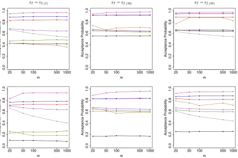
Fig. 1 Birth–death model. Empirical acceptance probability againstmwithT=1 (1st row) andT=2 (2nd row). The results are based on 100 K iterations of a Metropolis–Hastings independence sampler.BlackMDB,brownLB,redRB,blueRB−,greyGP-N,greenGP-S,purpleGP,pink

GP-MDB

found by repeatedly applying the Euler–Maruyama

approx-imation to (29) with a small time-step. To allow for different

inter-observation intervals, we take T ∈ {1,2}. An initial

condition ofx0 =50 and parameter valuesθ =(0.1,0.8)

gives (x1,(5),x1,(50),x1,(95)) = (18.49,24.62,31.68) and

(x2,(5),x2,(50),x2,(95))=(6.97,12.00,18.35).

Since the ODE system governing the LNA is tractable for this example, there is little difference in CPU cost between the

bridges (see Table1). Therefore, we use statistical efficiency

(as measured by empirical Metropolis–Hastings acceptance probablity) as a proxy for overall efficiency of each bridge, with higher probabilities preferred.

Figure1shows empirical acceptance probabilities against

the number of sub-intervals m for each bridge and each

xT. Figures2and3 compare 95 % credible regions of the

con-MDB

0.0 0.2 0.4 0.6 0.8 1.0

25

30

35

40

45

50

Xt

Time

RB

0.0 0.2 0.4 0.6 0.8 1.0

25

30

35

40

45

50

Xt

Time

LB,γ=0.0025

0.0 0.2 0.4 0.6 0.8 1.0

25

30

35

40

45

50

Xt

Time

GP-N

0.0 0.2 0.4 0.6 0.8 1.0

25

30

35

40

45

50

Xt

Time

GP-S

0.0 0.2 0.4 0.6 0.8 1.0

25

30

35

40

45

50

Xt

Time

GP

0.0 0.2 0.4 0.6 0.8 1.0

25

30

35

40

45

50

Xt

Time

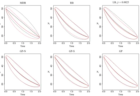
Fig. 2 Birth–death model. 95 % credible region (dashed line) and mean (solid line) of the true conditioned process (red) and various bridge constructs (black) usingxT =x1,(50)

ditioned process (obtained from the output of the Metropolis– Hastings independence sampler). It is clear from the figures

that asTis increased, the MDB fails to adequately account for

the nonlinear behaviour of the conditioned process. Indeed, in terms of empirical acceptance rate, MDB is outperformed

by all other bridges forT = 2. Asm is increased so that

the discretisation gets finer, the acceptance rates under all bridges (with the exception of GP-N) stay roughly constant.

For GP-N, the acceptance rates decrease withmwhenxT is

either the 5 or 95 % quantile ofXT|X0=50. In this case, the

variance associated with the approximate transition density

either overestimates (whenxT is the 5 % quantile) or

under-estimates (whenxT is the 95 % quantile) the true variance at

the end-point. For example, whenxTis the 95 % quantile, this

results (see Fig.3) in a ‘tapering in’ of the proposal relative to

the true conditioned process. GP-S, GP and LB give similar performance, although we note that GP-S and LB perform

particularly poorly whenxT is the 5 % quantile. Moreover,

LB requires the specification of a tuning parameterγ and

we found that the acceptance rate was fairly sensitive to the

choice ofγ. In all scenarios, RB, RB−and GP-MDB

compre-hensively outperform all other bridge constructs. WhenxT is

the median ofXT|X0=50, we see that RB and RB−(red and

blue lines in Fig.1) give near identical performance, withηt

adequately accounting for the observed nonlinear dynamics. In terms of statistical efficiency, GP-MDB outperforms both

RB and RB−in all scenarios, although the relative difference

is small.

4.2 Lotka–Volterra

In this example we consider a Lotka–Volterra model of

pred-ator-prey dynamics. We denote the system state at time t

byXt =(X1,t,X2,t), ordered as prey, predators. The

mass-action SDE representation of system dynamics takes the form

d Xt =

θ1X1,t−θ2X1,tX2,t

θ2X1,tX2,t−θ3X2,t dt

+

θ1X1,t+θ2X1,tX2,t −θ2X1,tX2,t −θ2X1,tX2,t θ3X2,t+θ2X1,tX2,t

1 2

d Wt.

MDB

0.0 0.5 1.0 1.5 2.0

20

30

40

50

Xt

Time

RB

0.0 0.5 1.0 1.5 2.0

20

30

40

50

Xt

Time

LB,γ=0.0025

0.0 0.5 1.0 1.5 2.0

20

30

40

50

Xt

Time

GP-N

0.0 0.5 1.0 1.5 2.0

20

30

40

50

Xt

Time

GP-S

0.0 0.5 1.0 1.5 2.0

20

30

40

50

Xt

Time

GP

0.0 0.5 1.0 1.5 2.0

20

30

40

50

Xt

Time

Fig. 3 Birth–death model. 95 % credible region (dashed line) and mean (solid line) of the true conditioned process (red) and various bridge constructs (black) usingxT =x2,(95)

Table 2 Lotka–Volterra model. Quantiles ofXT|X0=(71,79) found by repeatedly simulating from the Euler–Maruyama approximation of (30) with θ=(0.5,0.0025,0.3)

T=1 T=2 T=3 T =4

xT,(5) (82.47, 62.78) (107.35, 57.95) (142.00, 60.02) (185.04, 71.23)

xT,(50) (96.82, 71.93) (133.35, 70.75) (182.64, 77.36) (242.08, 97.23)

xT,(95) (112.13, 81.58) (162.28, 84.63) (228.82, 97.12) (308.58, 128.76)

The components ofθ = (θ1, θ2, θ3)can be interpreted as

prey reproduction rate, prey death and predator reproduc-tion rate, and predator death. Note that the ODE system

((17), (22) and (23)) governing the linear noise

approxi-mation of (30) is intractable and we therefore use the R

packagelsodato numerically solve the system when

nec-essary.

Following Boys et al. (2008) we impose the

parame-ter valuesθ = (θ1, θ2, θ3) = (0.5,0.0025,0.3) and let

x0=(71,79). We assume thatxT is known and generate a

number of challenging scenarios by takingxT as either the

5, 50 or 95 % marginal quantiles ofXT|X0 =(71,79)for

T ∈ {1,2,3,4}. These quantiles are shown in Table2. Note

that for this parameter choice, the expectation of Xt|X0 =

(71,79) is approximately periodic with a period around

17.

We fixed the discretisation by takingm = 50, but note

no appreciable difference in results for finer discretisations

(e.g.m=1000). As in the previous example, GP-N and GP-S

perform relatively poorly, therefore in what follows we omit these bridges from the results. Note that we include MDB for

reference. Figure4shows empirical acceptance probabilities

against T for each bridge and eachxT. Figure5compares

95 % credible regions of the proposal under various bridging strategies with the true conditioned process (obtained from the output of the Metropolis–Hastings independence sam-pler).

Unsurprisingly, asTis increased, MDB fails to adequately

account for the nonlinear behaviour of the conditioned process. LB offers a modest improvement (except when

xT = xT,(5)) but is generally outperformed by the other

xT=xT,(5)

0.0

0.2

0.4

0

.6

0.8

1.0

Acceptance Probability

Time

1 2 3 4

xT=xT,(50)

0.0

0.2

0.4

0

.6

0.8

1.0

Acceptance Probability

Time

1 2 3 4

xT=xT,(95)

0.0

0.2

0.4

0

.6

0.8

1.0

Acceptance Probability

Time

1 2 3 4

Fig. 4 Lotka–Volterra model. Empirical acceptance probabilities againstT. The results are based on 100 K iterations of a Metropolis–Hastings independence sampler.BlackMDB,brownLB,redRB,blueRB−,purpleGP,pinkGP-MDB

RB

0.0 0.2 0.4 0.6 0.8 1.0

70

75

80

85

X2

Time

RB−

0.0 0.2 0.4 0.6 0.8 1.0

70

75

80

85

X2

Time

LB,γ=0.01

0.0 0.2 0.4 0.6 0.8 1.0

70

75

80

85

X2

Time

0 1 2 3 4

60

80

100

120

X2

Time

0 1 2 3 4

60

80

100

120

X2

Time

γ=0.1

0 1 2 3 4

60

80

100

120

X2

Time

Fig. 5 Lotka–Volterra model. 95 % credible region (dashed line) and mean (solid line) of the true conditioned predator componentX2,t|x0,xT (red) and various bridge constructs (black) usingxT =xT,(95)withT=1 (1st row) andT =4 (2nd row)

required larger values of γ, reflecting the need for more

weight to be placed on the myopic component of the

con-struct. As for the previous example, unlessxT is the median

ofXT|x0, RB is comprehensively outperformed by RB−(see

Fig.5for the effect of increasingT on RB and RB−).

How-ever, we see that the acceptance probabilities are decreasing

inTfor both constructs. As noted byFearnhead et al.(2014),

the LNA can become poor as T increases, with the

impli-cation here being that the approximation of the expected

We note that the estimated acceptance probabilities are roughly constant for GP and (to a lesser extent) GP-MDB, and in terms of statistical efficiency for a fixed number of iterations, GP-MDB should be preferred over all other algo-rithms considered in this article. However, the difference in estimated acceptance probabilities between GP-MDB and

RB−is fairly small, even whenT =4 (e.g. 0.857 vs 0.577

whenxT =xT,(5)and 0.834 vs 0.606 whenxT =xT,(50)).

We also note that a Metropolis–Hastings scheme that uses

RB or RB− is some 30 times faster than a scheme with

GP or GP-MDB, since the latter require solving the LNA

ODE system for each sub-interval[τk,T]to maintain

rea-sonable statistical efficiency for a givenm. Therefore, we

further compare RB, RB−, GP and GP-MDB by computing

the minimum effective sample size (ESS) at timeT/2 (where

the minimum is over each component of XT/2) divided by

CPU cost (in seconds). We denote this measure of overall

efficiency by ESS/s. WhenxT = xT,(5) andT =1, ESS/s

scales roughly as 1:3 : 56: 83 for GP : GP-MDB : RB :

RB−. WhenT =4, ESS/s scales roughly as 1: 3:1 :17.

Hence, for this example, RB−is to be preferred in terms of

overall efficiency, although the relative difference between

RB− and GP-MDB appears to decrease as T is increased,

consistent with the behaviour of the empirical acceptance

rates observed in Fig.4.

4.3 Aphid growth

Matis et al. (2008) describe a stochastic model for aphid

dynamics in terms of population size (Nt) and cumulative

population size (Ct). The diffusion approximation of their

model is given by

d Nt

dCt =

θ1Nt−θ2NtCt

θ1Nt dt

+

θ1Nt+θ2NtCt θ1Nt

θ1Nt θ1Nt

1/2

d Wt (31)

where the components ofθ =(θ1, θ2)characterise the birth

and death rate respectively.Matis et al.(2008) also provide

a dataset consisting of cotton aphid counts recorded at times

t=0,1.14,2.29,3.57 and 4.57 weeks, and collected for 27

different treatment block combinations. The analysis of these data via a stochastic differential mixed-effects model driven

by (31) is the focus ofWhitaker et al.(2015).

Driven by the real data of Matis et al. (2008) and to

illustrate the proposed methodology in a challenging partial

observation scenario, we assume thatXTcannot be measured

exactly. Rather, we observe

YT =FXT +T, T|Σ∼N(0, Σ),

Table 3 Aphid growth model. Quantiles of Y3.57|X2.29 = (347.55,398.94) found by repeatedly simulating from the Euler– Maruyama approximation of (31) with θ = (1.45,0.0009), and corruptingN3.57with additiveN(0, σ2)noise

σ=5 σ=10 σ=50

y3.57,(5) 726.75 724.57 762.36

y3.57,(50) 786.09 815.51 774.41

y3.57,(95) 841.82 856.36 910.86

where Σ = σ2 _{andF = (1,0) so that only noisy}

obser-vation of NT is possible, and CT is not observed at all.

We consider a single treatment-block combination and con-sider the dynamics of the process over an observation time

interval [2.29,3.57], over which nonlinear dynamics are

typically observed. We fix θ and x2.29 at their marginal

posterior means found by Whitaker et al. (2015), that is,

atθ = (1.45,0.0009) andx2.29 = (347.55,398.94). We

generate various end-point conditioned scenarios by taking

y3.57to be either the 5, 50 or 95 % quantile ofY3.57|X2.29 =

(347.55,398.94), σ. To investigate the effect of

measure-ment error, we further takeσ ∈ {5,10,50}. The resulting

quantiles are shown in Table3. As with the previous example,

the ODE system governing the linear noise approximation of

(31) is intractable and we again use thelsodapackage to

numerically solve the system when necessary.

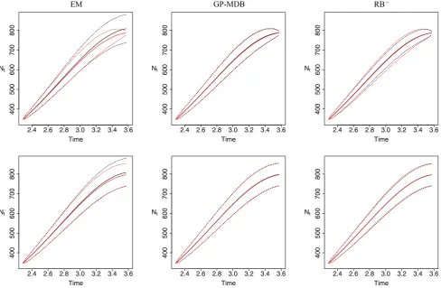
Figure6shows empirical acceptance probabilities against

σ for EM, RB, RB−, GP and GP-MDB. Figure7compares

95 % credible regions for a selection of bridges with the true conditioned process (obtained from the output of the

inde-pendence sampler). All results are based on m = 50 (but

note that no discernible difference in output was obtained for finer discretisations). As illustrated by both figures, the myopic sampler (EM) performs poorly (in terms of statistical efficiency, as measured by empirical acceptance probability)

when the measurement error variance is relatively small (σ =

5). Forσ =50, the performance of EM is comparable with

the other bridge constructs. In fact, asσincreases, the bridge

constructs coincide with the Euler–Maruyama approxima-tion of the target process. The gain in statistical performance

of RB− over RB is clear. Likewise, GP-MDB outperforms

GP, although the difference is very small forσ = 50 and

again we note that asσ increases, the variance under

GP-MDB,ΨMDB(xτk), approaches the Euler–Maruyama variance,

as used in GP.

The relative computational cost of each scheme can

be found in Table 1. EM is particularly cheap to

imple-ment, given the simple form of the construct and the M-H acceptance probability. However, this approach cannot be

recommended in this example forσ <10, due to its dire

sta-tistical efficiency. The computational cost of RB, RB−, GP

propos-y3.57=y3.57,(5)

0.0

0.2

0.4

0.6

0.8

1.0

Acceptance Probability

σ

0 5 0

1 5

y3.57=y3.57,(50)

0.0

0.2

0.4

0.6

0.8

1.0

Acceptance Probability

σ

0 5 0

1 5

y3.57=y3.57,(95)

0.0

0.2

0.4

0.6

0.8

1.0

Acceptance Probability

σ

0 5 0

1 5

Fig. 6 Aphid growth model. Empirical acceptance probabilities againstσ. The results are based on 100 K iterations of a Metropolis–Hastings independence sampler.TurquoiseEM,redRB,blueRB−,purpleGP,pinkGP-MDB

EM

2.4 2.6 2.8 3.0 3.2 3.4 3.6

400

500

600

700

800

Nt

Time

GP-MDB

2.4 2.6 2.8 3.0 3.2 3.4 3.6

400

500

600

700

800

Nt

Time

RB−

2.4 2.6 2.8 3.0 3.2 3.4 3.6

400

500

600

700

800

Nt

Time

2.4 2.6 2.8 3.0 3.2 3.4 3.6

400

500

6

00

700

8

00

Nt

Time

2.4 2.6 2.8 3.0 3.2 3.4 3.6

400

500

6

00

700

8

00

Nt

Time

2.4 2.6 2.8 3.0 3.2 3.4 3.6

400

500

6

00

700

8

00

Nt

Time

Fig. 7 Aphid growth model. 95 % credible region (dashed line) and mean (solid line) of the true conditioned aphid population component

Nt|x2.29,y3.57(red) and various bridge constructs (black) usingy3.57=y3.57,(50)withσ=5 (1st row) andσ=50 (2nd row)

als, we found that a naive implementation that only solves the LNA ODEs once, gave no appreciable difference in empirical acceptance probability as obtained when repeatedly solving

the ODE system for each sub-interval[τk,T](as is required

in the case of no measurement error). Consequently, in this

example, GP-MDB outperforms RB−in terms of overall

effi-ciency.

5 Discussion

the process into a deterministic part that accounts for forward dynamics, and a residual stochastic process. The intractable end-point conditioned residual SDE is approximated using

the modified diffusion bridge ofDurham and Gallant(2002).

Using three examples, we have investigated the empirical performance of two variants of the residual bridge. The first constructs the residual SDE by subtraction of a determinis-tic process based on the drift governing the target process (denoted RB). The second variant further subtracts the lin-ear noise approximation (LNA) of the expected conditioned

residual process (denoted RB−). Our examples included a

scenario in which the LNA system is tractable, and another where the system must be solved numerically. An example that considers partial and noisy observation of the process at a future time was also presented.

5.1 Choice of residual bridge

We find that for all examples considered, the residual bridge that further subtracts the LNA mean results in improved sta-tistical efficiency (over the simple implementation based on the drift subtraction only) at the expense of having to solve

a larger ODE system consisting of orderd2 equations (as

opposed to just d when using the simpler variant). For a

known initial time-pointx0, the ODE system need only be

solved once, irrespective of the number of skeleton bridges required. Taking the Lotka–Volterra diffusion (described in

Sect.4.2) as an example, overall efficiency (as measured by

minimum effective sample size per second, ESS/s, at time

T/2) of RB− is 1.5 times that of RB when T = 1 and

xT is either the 5 or 95 % quantile of XT|x0. This factor

increases to 17 when T = 4. However, for unknown x0,

as would typically be the case when performing parameter inference, the ODE solution will be required for each skele-ton bridge, and the difference in computational cost between the two approaches is likely to be important, especially as the dimension of the state space increases. For the Lotka– Volterra example, the computational cost for solving the ODE

systemfor each bridgescales as 1:2.8 for RB : RB−.

There-fore, the relative difference in ESS/s would reduce to a factor

of roughly 0.5 whenT =1 (so that RB would be preferred)

and 6 when T = 4. We therefore anticipate that in

prob-lems wherex0is unknown, the simple residual bridge is to

be preferred, unless the ODE system governing the LNA is

tractable, or the dimensiond of Xt is relatively small, say

d<5.

5.2 Residual bridge or guided proposal?

We have compared the performance of our approach to sev-eral existing bridge constructs (adapting where necessary to the case of noisy and partial observation). These include the

modified diffusion bridge (Durham and Gallant 2002),

Lind-ström bridge (Lindström 2012) and guided proposal (Schauer

et al. 2016). Our implementation of the latter uses the LNA to guide the proposal. We find that a further modification that replaces the Euler–Maruyama variance with the MDB variance gives a particularly effective bridge, outperforming all others considered here, in terms of statistical efficiency.

We find that for fixed x0 and noisy observation of xT, an

efficient implementation of the guided proposal is possi-ble, where the ODE system governing the LNA need only be solved once. In this case, the guided proposal outper-forms both implementations of the residual bridge in terms of overall efficiency. However, we found that in the case

of no measurement error (so thatxT is known exactly), the

guided proposal required that the ODEs governing the LNA be re-integrated for each intermediate time-point and for each skeleton bridge required. Unless the ODE system can be solved analytically, we find that when combining statistical and computational efficiency, the guided proposal is outper-formed by both implementations of the residual bridge.

5.3 Extensions

Our work can be extended in a number of ways. For exam-ple, it may be possible to improve the statistical performance of the residual bridges by replacing the Euler–Maruyama

approximation of the variance ofYT|X0with that obtained

under the LNA. This approach could also be combined with the Lindström sampler to avoid specification of a tuning

parameter. Deriving the limiting (as τ → 0) forms of

the Metropolis–Hastings acceptance rates associated with the residual bridges would be problematic due to the time dependent terms entering the variance of the constructs. Nev-ertheless, this merits further research. Interest also lies in the comparison of the bridge constructs for SDEs that exhibit multimodal behaviour, although we anticipate that further modification of the constructs will be required to efficiently deal with such a scenario.

Acknowledgments The authors would like to thank the associate edi-tor and three anonymous referees for their suggestions for improving this paper.

Open Access This article is distributed under the terms of the Creative Commons Attribution 4.0 International License (http://creativecomm ons.org/licenses/by/4.0/), which permits unrestricted use, distribution, and reproduction in any medium, provided you give appropriate credit to the original author(s) and the source, provide a link to the Creative Commons license, and indicate if changes were made.

References