warwick.ac.uk/lib-publications
Original citation:
Saginbekov, Sain and Jhumka, Arshad. (2017) Many-to-many data aggregation scheduling in
wireless sensor networks with two sinks. Computer Networks, 123 . pp. 184-199.
Permanent WRAP URL:
http://wrap.warwick.ac.uk/88734
Copyright and reuse:
The Warwick Research Archive Portal (WRAP) makes this work by researchers of the
University of Warwick available open access under the following conditions. Copyright ©
and all moral rights to the version of the paper presented here belong to the individual
author(s) and/or other copyright owners. To the extent reasonable and practicable the
material made available in WRAP has been checked for eligibility before being made
available.
Copies of full items can be used for personal research or study, educational, or not-for-profit
purposes without prior permission or charge. Provided that the authors, title and full
bibliographic details are credited, a hyperlink and/or URL is given for the original metadata
page and the content is not changed in any way.
Publisher’s statement:
© 2017, Elsevier. Licensed under the Creative Commons
Attribution-NonCommercial-NoDerivatives 4.0 International
http://creativecommons.org/licenses/by-nc-nd/4.0/
A note on versions:
The version presented here may differ from the published version or, version of record, if
you wish to cite this item you are advised to consult the publisher’s version. Please see the
‘permanent WRAP url’ above for details on accessing the published version and note that
access may require a subscription.
Many-to-Many Data Aggregation Scheduling in Wireless Sensor Networks with
Two Sinks
Sain Saginbekova,∗, Arshad Jhumkab
aDepartment of Computer Science, Nazarbayev University, Astana, Kazakhstan bDepartment of Computer Science, University of Warwick, Coventry CV4 7AL, UK
Abstract
Traditionally, wireless sensor networks (WSNs) have been deployed with a single sink. Due to the emergence of
sophisticated applications, WSNs may require more than one sink. Moreover, deploying more than one sink may
prolong the network lifetime and address fault tolerance issues. Several protocols have been proposed for WSNs
with multiple sinks. However, most of them are routing protocols. Differently, our main contribution, in this paper,
is the development of a distributed data aggregation scheduling (DAS) algorithm for WSNs with two sinks. We
also propose a distributed energy-balancing algorithm to balance the energy consumption for the aggregators. The
energy-balancing algorithm first forms trees rooted at nodes which are termedvirtual sinks and then balances the
number of children at a given level to level the energy consumption. Subsequently, the DAS algorithm takes the
resulting balanced tree and assigns contiguous slots to sibling nodes, to avoid unnecessary energy waste due to
frequent active-sleep transitions. We prove a number of theoretical results and the correctness of the algorithms.
Through simulation and testbed experiments, we show the correctness and performance of our algorithms.
Keywords: Wireless sensor networks, Data aggregation scheduling, Two sinks, Many-to-many communication,
Medium access control
1. INTRODUCTION
A wireless sensor network (WSN) consists of a set of resource-constrained nodes, that communicate wirelessly.
These nodes sense the environment for events of interest and subsequently relay the information to a dedicated
device calledsink, with data from several nodes aggregated along the way for energy efficiency reasons. The data
can then later be analysed offline.
Traditionally, WSNs have been deployed with a single sink [1]. However, there are several reasons that limit the
usefulness of a single sink. The emergence of more sophisticated applications, such as Heating, Ventilation, and Air
Conditioning (HVAC) systems [28], requires WSNs with more than one sink. Moreover, the deployment of more
than one sink may improve the network throughput and prolong network lifetime by balancing energy consumption,
∗Corresponding author
Email addresses: [email protected](Sain Saginbekov),[email protected](Arshad Jhumka)
and may address fault tolerance issues [25, 42, 36].
WSNs are typically resource-constrained networks, with nodes having limited computational and energy
re-sources. To reduce energy consumption, various approaches exist, such as duty-cycling and the use of appropriate
medium access control (MAC) protocols. Major sources of energy waste at the MAC layer are:
• Message collisions, which require the retransmission of the collided packets,
• Message overhearing, where a node receives a message meant for another node, and
• Idle listening, which means that a node keeps on listening for messages on an otherwise idle channel [44].
To address the above problems, a typical solution is to use a Time Division Multiple Access (TDMA) based
MAC protocol. TDMA MAC protocols work by dividing time into slots and assigning those slots to nodes. Each
node can then only transmit in a slot to which it has been assigned. Several TDMA-based MAC protocols have
been proposed for WSNs, e.g., [31, 32, 37]. However, most of them have been developed for a WSN with a single
sink. Thus, there is a need for TDMA-based MAC protocols specifically designed for WSNs with multiple sinks.
However, there is a dearth of work in this area. Data aggregation scheduling (DAS) algorithms in a WSN with
multiple sinkshave been presented in [21, 3]. However, in these works, the data aggregation scheduling is done from
many nodes to one sink which collects all the messages, whereas this work considers data aggregation scheduling
frommany nodes tomany sinks, where every sink has to collect all messages.
The way we propose to solve the data aggregation scheduling problem in WSNs with two sinks is to first
develop a backbone that connects the two sinks and then allocate slots to nodes that connect to the backbone.
The problem of developing the backbone, i.e., a path connecting the sinks, is directly related to the problem of
developing a (minimum) Steiner tree [11], which is a well-studied combinatorial optimization problem. Given a
graph G= (V, E) with weighted edges and a set of nodesS ⊆V, a Steiner tree T interconnects all elements in S
such that the sum of the edge weights inT is minimal. In the general case, this is an NP-complete problem [20].
The minimum Steiner tree problem can be seen as a combination of computing shortest paths and of computing
spanning trees. If the number of vertices to be joined is two, then we only need to compute the shortest path. On
the other hand, if all the vertices are involved, then a spanning tree is computed. In this paper, as we focus on two
sinks, we will construct a shortest path, which can be achieved in polynomial-time.
In this context, we make the following novel contributions:
• In Section 4, we formalise the problem of DAS scheduling in a WSN with two sinks, where data needs to reach
both sinks.
• In Section 5, we prove an impossibility1result, as well as derive a lower bound for solving weak DAS, a special
case of DAS.
• In Section 6, we propose two algorithms which, taken together, solve weak DAS for two sinks. The output of
the combined algorithms is a schedule that matches the predicted lower bound.
• Through both simulation and testbed experiments, we show the performance and correctness of the algorithms
in Section 8.
The other parts are as follows: In Section 2, we present an overview of related work. We present the formal basis
of our work in Section 3. In Section 7, we present the experimental setup. We conclude the paper in Section 9.
2. RELATED WORK
A data aggregation technique is used in data gathering in WSNs to reduce energy consumption, as it reduces
the number of transmissions [22]. A number of data aggregation protocols have been proposed in the literature [14,
45, 34, 12, 47, 23, 38, 27]. The routing structure of these protocols could be tree-based [38, 34, 12, 23],
cluster-based [14, 45], chain-cluster-based [27], and grid-cluster-based [19, 30]. However, these protocols have been proposed for WSNs
with a single sink. Although our proposed protocol is developed for WSNs with two sinks, the routing structure of
our proposed protocol is based on a tree structure.
Protocols that have been developed for communication in WSNs with multiple sinks can be found in [5, 28, 21,
3, 39, 41, 48, 6, 13, 24]. The authors of [5] developed an algorithm where a node chooses a sink in a multi-sink WSN
to send its data in such a way that it minimizes energy consumption. A scheme proposed in [28] performs data
collection from many nodes to many sinks, i.e., many-to-many communication. The main idea of the protocol is to
reduce the number of redundant transmissions by leveraging neighbourhood information. An algorithm that builds
two node-disjoint paths from every node to two different sinks was proposed in [39]. If one of the two paths fails, the
other path is used to route the data. In [41], the authors propose a routing protocol that is using a hexagon-based
architecture. The nodes in the network are grouped into hexagons, based on their locations. The routing protocol
proposed in [48], is based on trees. In the protocol, different trees rooted at different sinks are used to forward
data. The authors of [6] have proposed an online algorithm for data collection in WSNs with multiple sinks, where
sinks are deployed in a stepwise fashion during network operation. In [29], the authors present different routing
schemes that are based on a logical tree structure, which is built based on the residual energy of each node. One of
these schemes uses a secondary sink to maximize the network lifetime. A data reporting algorithm used for object
tracking in multi-sinks WSNs was presented in [10]. The algorithm attempted to reduce energy consumption and
balance the load among sinks and nodes.
The works presented in [21, 3, 13, 24] are more closely related to the work presented in this paper. In [21],
in addition to an algorithm that computes the shortest-path trees rooted at each sink in a multi-sinks WSN, the
authors proposed a scheduling algorithm that uses a graph colouring technique. Then, a node will send messages to
in multi-sinks WSNs. One of the algorithms is a Voronoi-based scheduling algorithm, where the sensing area is
divided into regions to formkforests, one forest for each sink. Subsequently, the algorithm computes the schedules
for the nodes. In [13] and [24], the authors proposed cross-layer schemes that consider the routing as well as the
MAC layer to maximize the network lifetime and reduce the latency respectively. Most of the above protocols
either developed appropriate routing protocols for multi-sinks WSNs or the techniques involved a subset of the
nodes forwarding messages to a single sink only. In contrast, we consider the case where many nodes send their
data totwo sinks, which is an instance of many-to-many communication.
3. SYSTEM MODEL
We provide the necessary formal background, including the models we use, the syntax we use to write the
algorithms and the associated semantics, the computation and communication models.
3.1. Topology and processes
Communication in WSNs is typically modeled a circular communication range centered on a node, and it is
typically assumed that all nodes have the same communication range. With this model, a node is thought to be able
to directly exchange data with all devices within its communication range. In graph-theoretic terms, we represent
a WSN as a undirected graph G = (V, E) with a set V of vertices representing the nodes, and a set E of edges
(or links) representing the communication links between pairs of nodes. A path between two nodesn1 andni is a
sequence of nodes γ=n1·n2. . . ni such that∀j,1≤j < i,(nj, nj+1)∈E. We assume a network where no node
has both sinks as neighbours. We also assume that the network topology remains constant, i.e., there is no node
crash and no link failure.
A program consists of a finite set of processes. Each process contains a finite set of variables, each taking values
from a given finite domain, and a finite set of actions. An assignment of values to variables is called a state and
the set of value assignments denote the state space of the program. A predicate defines a set of states, such that
the predicate evaluates totrue in these states.
3.2. Program syntax and semantics
We write programs in a style similar to the guarded command notation [7]. An action has the form
state = X
uponhguardi
command
The program is written in such a way that it encodes an automaton that captures the execution of the program.
Thestate variable indicates the (automaton) state the program is in, i.e., (X) (which we refer to as the Astate),
given state, theguard, which is a predicate defined over the set of variables of a process, is evaluated. If it is true,
then the correspondingcommand is executed. When the command is executed, the state of the program changes.
If thestate variable changes too, then the Astate of the program changes. When the guard is true, then we say
that the action is enabled. A process is enabled in a stateswhen at least one of its guards is enabled ins.
Acommand is a sequence of assignments and branching statements. A guard or command can contain universal
or existential quantifiers of the form: hquantif ierihboundvariablesi:hrangei:htermi, whererange andterm are
Boolean constructs. A special timeout(timer) guard evaluates to true when a timer variable reaches zero. A
set(timer,value) command sets the timer variable to a specified value.
We choose this programming style for several reasons. First, it is usually simpler to formally reason on a program
execution in terms of what guards become true at a given point (i.e., state) in the execution, rather than following
a specific control flow. Moreover, representing a program as such makes programs more compact, compared to the
more traditional state transition or procedural representations. Finally, this notation matches the programming
style of many WSN software platforms, which tend to be event driven [15]. In these cases, the binding of events to
their handlers2is, in a sense, corresponding to the evaluation of guards.
The execution of a command of a program A causes the program to update one or more variables and moves
the program from one state to another in one atomic step. In a given state s, several processes may be enabled,
and a decision is needed about which one(s) to execute. The subset of processes that take a step when possible is
chosen according to different scheduling policies. To ensure the system makes progress, a notion of fairness is also
required. Whenever any of the enabled processes can take a step independent of all others, that is, a continuously
enabled action is eventually executed, we say the system is weakly fair [9] and runs in an asynchronous manner.
This entails there isno bound on relative process speeds and message transmission time.
3.3. Communication
Each process is linked with an (auxiliary)channel variable, denoted bych, modeling a FIFO queue of incoming
messages sent by other processes. The domain of thechvariable is the set of (possibly infinite) message sequences.
An action with a rcv(msg,sender) guard is enabled when there is a message at the head of the channel variable
ch of a process. Executing the corresponding command causes the message at the head of the channel to be
dequeued, whilemsg andsender are bound to the content of the message and the sender identifier. Differently, the
send(type,src,dest,msg) command causes the messagemsg to be attached to the tail of the channel variablechof
process(es) in thedest set. To capture the broadcast multi-hop nature of WSNs, we extend the semantics of send
with abcast command, with the following syntax: bcast(type,msg). The bcast command causes themsg to be
simultaneously appended to the tail of the channel variable of all nodes that are within the communication range
of the sender. We assume communication to be reliable, i.e., channels always deliver messages placed on them.
4. PROBLEM FORMULATION
We present the following definitions that will be used in this paper.
Definition 1(Schedule). A scheduleS:V →2Nis a function that maps a node to a set of time slots (represented
as natural numbers).
Definition 2 (DAS-label). Given a networkG= (V, E), a sink ∆, a schedule S and a path γ=n·m . . .∆, we
say that n is DAS-labeled under S onγfor ∆ if∃t∈ S(n)· ∃t0 ∈S (m) :t0> t.
We call the node m onγ the ∆-parent ofnand γ the DAS-path forn. A node is DAS-labeled if its parent is
assigned at least a later time slot, i.e., a slot with higher value.
Definition 3(Strong and Weak schedule). Given a networkG= (V, E), a sink ∆∈V and a scheduleS,Sis said
to be a strong DAS schedule w.r.t. ∆for a node n∈V iff∀pathγi=n·mi. . .∆,nis DAS-labeled underS onγi
for∆. S is a weak DAS schedule w.r.t. ∆fornif ∃path γ=n·mi. . .∆ such thatnis DAS-labeled under S on
γ for∆.
A schedule S is strong DAS (resp. weak DAS) for G iff∀n∈V, S is strong DAS schedule (resp. weak DAS
schedule) for∆ forn.
The difference between a weak and a strong DAS schedule is that a weak DAS schedule requires a node to be
DAS-labeled w.r.t to a single path to the sink whereas a strong one requires a node to be DAS-labeled for every
path. We will only say a strong or weak schedule whenever ∆ is obvious from the context. A strong schedule,
in essence, is resilient to problems that occur in the network such as unreliable radio links or node crashes during
deployment. On the other hand, a weak schedule is not resilient and, any problem happening, will entail that a
message between two neighbour nodes may be lost.
It has been shown in [17] that it is impossible to develop strong schedules. Given a network with 2 sinks ∆1,∆2,
we then wish to develop a weak schedule for ∆1 and ∆2. There are several possibilities to achieve this. In general,
to develop a weak schedule, several works have adopted the approach whereby a tree is first constructed, rooted at
the sink, and then slots assigned along the branches to satisfy the data aggregation constraints. A trivial solution
is to construct two trees, each rooted at a sink, and then to assign slots to nodes along the trees. This means that
nodes can have two slots, i.e., meaning that nodes may have to do two transmissions for the same message. Thus,
we seek to reduce the number of slots for nodes to transmit in.
4.1. DAS Scheduling
We capture slots assignment with a set of decision variables.
tS n=
1, t∈ S(n)
The decision variable tS
n is set to 1 if slot t is one of the assigned slots to node n under scheduleS. A set of value assignment to these variables represent a possible schedule. The number of slots used, which is equal to the
number of transmission by nodes, has to be reduced for extending the lifetime of the network. The number of slots
used is given by:
numSlotsS= X t∈N,n∈V
tS
n. (1)
We also capture the number of nodes with multiple slots as follows:
fS n =
1, |S(n)|>1
0, otherwise.
However, such a schedule may not assign a slot to a given node, so we need to rule out some schedules by adding
a constraint:
∀n∈V,∃t:tS n= 1.
The above constraint means that all nodes in the network will be assigned at least one slot. We also rule out
schedulesS that assign the same slot to two nodes that are in the two-hop neighbourhood, i.e,
∀m, n∈V :tS
m= 1∧tSn= 1⇒ ¬2HopN(m, n),
where 2HopN(m, n) returns true if m and n are in each other’s two-hop neighbourhood. This can be done by
using information about two-hop neighbourhood, and it can be obtained by exchanging messages with neighbours.
Finally, we require to generate weak DAS schedulesS, i.e.,
∀m∈V · ∃n∈V,(m·n . . .∆1) :tSm= 1⇒ ∃τ > t:τnS= 1,
∀m∈V · ∃n∈V,(m·n . . .∆2) :tSm= 1⇒ ∃τ > t:τnS= 1.
To generate an energy-efficient collision-free weak DAS schedule for both ∆1and ∆2, there are different
possibil-ities. For example, one may seek to minimisenumSlots to reduce the number of slots during which nodes transmit.
Another possibility is to reduce the number of times any node can transmit, in some sort of load balancing. We
EECF-2-DAS optimization problem:
Obtain anS such that
minimiseP ∀t
P
∀n∈V fnS subject to
1. ∀n∈V · ∃t:tS n6= 0,
2. ∀m∈V · ∃n∈V,(m·n . . .∆1) :tSm= 1⇒ ∃τ > t:τnS= 1,
3. ∀m∈V · ∃n∈V,(m·n . . .∆2) :tSm= 1⇒ ∃τ > t:τnS= 1,
4. ∀m, n∈V :tS
m= 1∧tSn= 1⇒ ¬2HopN(m, n).
The EECF-2-DAS problem consists of two subproblems: (i) The first three conditions amount to what we call the
weak DAS problem for two sinks and (ii) the fourth condition ensures that any weak DAS schedule is collision-free.
5. FINDING LOWER AND UPPER BOUNDS
In this section, we investigate how small the number of nodes with multiple slots can be to generate an
energy-efficient collision-free weak schedule in a network with 2 sinks.
5.1. Every Node Has a Single Slot (P
∀n∈V fnS= 0)
In this section, we seek a lower bound on the number of nodes that can have multiple slots assigned to them.
As a starting point, we endeavour to determine whether every node can have only a single slot, and the result is
captured in Theorem 1.
Theorem 1 (Impossibility of 1 slot). Given a network G= (V, E)with 2 sinks ∆1,∆2, then there exists no weak
DAS scheduleS for∆1,∆2 such that P∀n∈VfnS= 0.
Proof. We assume there is such a weak DASSand then show a contradiction.
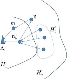
Given a networkGwith 2 sinks ∆1,∆2, we have part of the network as follows: Focusing on the sink ∆1, there
is a setH1 of nodes one hop away from it. There is also a setH2 of nodes two hops away from it. We also denote
byn1
h, the node inH1with the largest slot number. We also assume, for some set of nodesH20 ⊆H2, that all nodes
inH20 haven1
h as a ∆1-parent.
Since the schedule is weak DAS, then ∀n∈H2· ∃m∈H1 :S(m)>S(n)3. Also, because the schedule is weak
DAS, no node in H20 can be a ∆2-parent forn1h. Thus, there∃η ∈H2, η 6∈H20 such thatη is a ∆2-parent forn1h
and, given thatSis a weak DAS schedule, thenS(η)>S(n1h).
Now, sinceη ∈H2,∃m∈H1, m=6 n1hsuch thatmis a ∆1-parent forηand, given thatSis a weak DAS schedule,
thenS(m)>S(η). Since we assumed thatn1h has the largest slot in H1, it implies that∀m∈H2 :S(n1h)>S(m).
3Since
Figure 1: An illustration of the proof of Theorem 1
This also means thatS(η)<S(n1
h), which contradicts the previous conclusion thatS(η)>S(n
1
h). See Figure 1 for illustration.
Hence, no suchS exists.
Therefore, we have proved that there exists no algorithm that can generate a weak DAS schedule for both ∆1
and ∆2with all nodes being assigned a single slot. Theorem 1 captures a lower bound for developing a weak DAS
schedule for two sinks, in that it means that it is mandatory for some nodes to have at least two slots to solve weak
DAS for two sinks.
5.2. Towards Minimizing P ∀n∈VfnS
Having established that there should be a certain number of nodes that require at least two slots, an important
question is: how can these nodes with 2 slots be chosen optimally from the network?
Our approach to generating a schedule for two sinks is to first develop a network backbone and then to
subse-quently perform slot assignment. As the problem is related to the Steiner Tree problem, we only require to develop
a backbone between the two sinks, which in this case is the shortest path between the two sinks. Thus, one way of
building a network that solves the weak DAS problem for a two-sink WSN is to assign 2 slots to the nodes on the
shortest path that connects ∆1 and ∆2 and possibly assign 1 slot to all other nodes, as shown in Figure 2. The
(s+i) values in Figure 2 are the time slots assigned to the nodes and the arrows show the direction of packets sent
in time slot (s+i). Each node then transmits its message to one of its neighbours on the path. In turn, the nodes
on the path use 2 slots to send their aggregated values to the two sinks, one slot for each sink.
In the example, there are 5 nodes that have 2 slots. However, we can further reduce the number of nodes with
2 slots to 4 by assigning only one slot to the neighbor of either ∆1 or ∆2 on the shortest path. For example, in
Figure 2, the node with the slot number s+ 4 may not use its time slot s+ 5 as it can simultaneously send its
aggregated data to both its neighbors ((i) the sink and (ii) the node with slots (s+ 3,s+ 6)) in a single slot (i.e.,
s+ 4). Thus, the minimum number of nodes with at least two slots that can connect two sinks is captured in the
Figure 2: An example of network that solves weak DAS. Arrows show the sink to which the slot is related. sis an integer that shows the slot assigned to the node.
Figure 3: An illustration of the proof of Theorem 2.
Corollary 1. Given a network G = (V, E) with two sinks ∆1 and ∆2, then there exists a weak DAS S for G,
P
∀n∈V fnS=l−2, wherel is the length of the shortest path between∆1 and∆2.
Since we know that it is possible to obtain a weak DAS schedule S that assigns two or more slots to at most
l−2 nodes, the objective is to determine the minimum number of such nodes with at least 2 slots. This is captured
in the following result (Theorem 2):
Theorem 2. Consider a finite networkG= (V, E)with two sinks∆1and∆2, a pathP = ∆1·n1·n2. . . nl−1·∆2
that is a shortest path between ∆1 and∆2 of length l with l−1 nodes. Then, there exists no weak DAS schedule
S forGsuch thatP∀n∈V fnS≤l−3.
From Corollary 1, we know that it is possible to have a weak DAS schedule with at most l−2 nodes that
assigned more than 2 slots. Now, we prove that it is impossible to have such a schedule with less thanl−2 nodes.
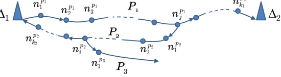
Proof. We show that to haveGwith at mostl−3 nodes that have at least 2 slots, Ghas to be infinite.
Let S1 be a set of nodes that have already sent once (used 1 time slot) and S2 be a set of nodes that have
already sent at least twice (used 2 time slots), where |S1| ≥ 0 and |S2| ≥ 0. Let P1 = np11, n
p1
2 , ..., n
p1
k1,∆2
be the path, of length k1 ≥ l−1, which delivers a packet of n1p1 to ∆2, where np11 is a neighbour of ∆1 and
S(np11)<S(n
p1
2 )< ... <S(n
p1
k1). See Figure 3 for illustration. After delivering the packet ofn
p1
1 to ∆2, the set S2
becomesS2=S2∪(P1∩S1), i.e., some nodes on path P1 could have sent one more time. Then,
[image:11.612.171.446.252.328.2](ii) Otherwise,S1=S1∪P1 and there exists a set of nodes onP1that sent only once. Letnpj1 be the node onP1
closest to ∆2 that has sent only once. Note that now|S2| ≥k1−j. As every node should send its packet to
both ∆1 and ∆2, there exists a path P2 =n
p1
j , n p2
1 , n
p2
2 , ..., n
p2
k2,∆1, of lengthk2+ 1, which delivers a packet
of np1
j to ∆1, where S(npj1)< S(n p2
1 ) <S(n
p2
2 ) < ... < S(n
p2
k2). After delivering the packet of n
p1
j to ∆1, if
|P2∩S1|=k2, i.e., all nodes onP2\n
p1
j have already sent at least twice, then we are done, as|S2| ≥k1−jand k2+k1−j ≥l−2. Otherwise, as in case(ii), the setsS2andS1becomeS2=S2∪(P2∩S1) andS1=S1∪P2.
And there exists a set of nodes onP2that sent only once,npi2 onP2that sent only once and is the closest node
to ∆1, andP3 that delivers a packet of npi2 to ∆2. The step continues infinitely many times if Gis infinite.
However, asGis finite the step continues until there exists a pathPrsuch that|S2∪(Pr∩S1)| ≥l−2.
6. ALGORITHMS
Based on the results developed in Section 5, we develop a 3-stage weak DAS algorithm for WSNs with two
sinks. The first phase computes a shortest path between the two designated sinks. Every node on the shortest
path is considered a virtual sink. The second phase consists of each virtual sink constructing a tree that satisfies
some property, e.g., balanced tree. This phase is explained in Section 6.2. The final phase assigns slots to nodes
in the network in such a way so as to satisfy a given property, e.g., minimum latency. This phase is explained in
Section 6.3.
In this paper, we will focus on the following properties: (i) we develop a balanced tree algorithm such that
nodes at a given level spend similar amount of energy and (ii) sibling nodes are allocated contiguous slots so that
a parent node does not require switching its radio on and off to capture the data of its children, thereby saving
energy [2, 35, 18].
6.1. Phase 1: Computing the Shortest Path Between the two Sinks
As our results show that a shortest path between the two sinks ∆1 and ∆2 is required to minimise the number
of nodes with more than a single slot, we first form a shortest pathP = ∆1·n1. . . nl·∆2 between ∆1 and ∆2.
After formingP, all nodes onP, apart from the two sinks, will take the role ofvirtual sinkand set their variables
to 1 andhop to 0. The reason the sinks are not virtual sinks is that they do not take part in data aggregation and
forwarding. The second phase of the algorithm, which we describe in Section 6.2, then starts.
6.2. Phase 2: Developing a Tree Structure
Once a shortest path has been obtained from the first phase, there now exists a set of “virtual sinks” in the
(a) Parent with smaller hop distance (b) Parent with smaller number of children
Figure 4: Parent selection
The first two phases of our algorithm are somewhat similar to the algorithm proposed in [16], where authors
propose an algorithm that forms a Greedy Incremental Tree (GIT)-like tree to perform energy-efficient in-network
data aggregation. Their algorithm consists of first forming a shortest path between the first source node to a sink
and then connecting all other source nodes to the path in a greedy fashion using hop number as a cost. The idea
behind building GIT-like tree is that it improves path sharing, i.e., it allows earlier data aggregation to reduce data
transmissions. However, their algorithm differs from ours in that their algorithm does not balance the number of
children while our algorithm does. The next section explains our balancing algorithm.
6.2.1. Balanced tree formation
In this section, we describe the balanced tree formation (BTF) algorithm that we adopt (See Figure 7). When
developing the balanced tree, we focus on two main parameters, in the following order: (i) a node chooses a parent
based on its (hop) distance from its virtual sink ancestor, in the sense that the node will choose to join a tree where
it is closer to a virtual sink, and (ii) if there are competing trees, then a node will join the tree that will make the
overall tree structure balanced among the nodes with the same hop distance.
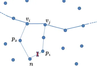
In other words, a node nwill select nodep2 over its current parentp1 only if
• p2 has a smaller hop distance (from a virtual sink) than that ofp1. Figure 4(a) illustrates this case.
• If both p1 and p2 are equidistant to a virtual sink, then n switches parent if p2 has a smaller number of
children. Figure 4(b) illustrates this case.
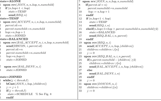
A node can be in one of five states: ALONE, TEMP, JOINED, BALANCED and SCHEDULE. Initially, all
virtual sinks are in the JOINED state, and all other nodes are in the ALONE state. A node goes to the TEMP
state when it finds a potential parent with a smaller hop distance. A node goes to the BALANCED state when it
finds a potential parent with a smaller number of children. In the TEMP or BALANCED state, a node waits for
some time to get a response from the potential parent.
Informally, the algorithm starts with the virtual sinks broadcasting (i.e., advertising) JOIN packets. When
distance ofn2. If the hop ofn2is smaller, thenn1 requestsn2to be its parent by sendingREQ packet, and setsn2
as its parent ifn1 receives anACCEPT packet from n2. If the hop numbers are equal and the number of children
ofn2 is at least two smaller than the number of children of its current parent, thenn1 requestsn2 to be its parent
by sending a REQ BALpacket. If n1 receives aBAL ACCEPT packet fromn2, it notifies its current parent, by
sending aDISCON packet, stating that it will connect to another parent. It then setsn2 as its parent. Whenever
n2 sendsACCEPT or BAL ACCEPT ton1, it addsn1 to itschildren set. Whenever a node receives aDISCON
packet from a noden, it removesnfrom itschildren set. When a node stops receiving any packet except JOIN, it
goes to theSCHEDULE state.
Lemma 1 shows that BTF algorithm correctly achieves this goal.
Lemma 1(Invariant of BTF). Given a networkG= (V, A)with two sinks∆1,∆2, then the following is an invariant
for the BTF algorithm in Figure 7:
∀m∈V \V S:
1. (m.parent6=⊥ ⇒m.hop6=∞)
2. (m.hop≤m.hop0)
3. [(m.parent06=m.parent)⇒((m.hop < m.hop0)∨((m.hop=m.hop0)∧(m.parent.numchild < m.parent0.numchild0)))]
The conditions mean the following: (i) The first states that ifparent is set (i.e, not undefined), then hopis set
too, (ii) hop cannot increase during execution and (iii) if parent changes, then either hop value decreases or the
node is joining a parent with a smaller number of children.
Proof. To prove that the above is an invariant, we show that it is satisfied in the initial state of the program and
subsequent action preserves the invariant (Note that the primed variable indicates the value from the previous
state).
The invariant is trivially satisfied in the initial state where parent=⊥ and hop =∞. In state ALONE, the
invariant is not violated as no state change occurs. In state TEMP, the value of hop decreases since a node m
receiveshACCEP Tifrom a nodenonly ifnhas a smaller hop (line 2 state ALONE, and line 12 state JOINED),
which preserves the invariant. In state TEMP, the value of the parent changes too as eitherm gets a new parent
with a smaller hop (line 12 state JOINED) or gets a parent for the first time (line 2 state ALONE), which preserves
the invariant. In state BALANCED, when node mreceives a hBAL ACCEP Ti message,m changes parent due
to m having a possible new parent with fewer children (state JOINED line 15). In state JOINED, when nodem
receives ahJ OINipacket, it updates its state based on that of its parent’s, which preserves the invariant.
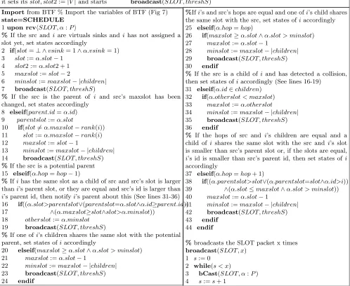
6.3. Phase 3: Slot Allocation for DAS Scheduling
Once the virtual sinks are obtained (phase 1) and each one has its own tree structure (phase 2), every node will
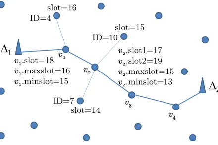
Figure 5: Scheduling example. The network has 20 nodes.v2 is the parent of the nodes with ID=10 and ID=7.v1 is the parent of the
node with ID=4.
6.3.1. Energy-Efficient Collision Free (EECF) DAS Algorithm for Balanced Tree
In this section, we propose a DAS algorithm that leverages the balanced tree obtained (see Section 6.2.1). To
make the DAS energy-efficient, we seek to assign contiguous slots to children so that a parent does not need to
continuously sleep and wake-up to collect data as this leads to unnecessary energy usage [2, 35, 18]. This energy
saving comes in addition to that obtained from duty cycling. Further, since the tree is balanced (at a given level),
then nodes at that level spend comparable amount of energy, without creating energy holes in the network (assuming
similar sensing loads).
We propose a weak DAS algorithm that works in a greedy fashion (see Figure 8). In the algorithm, every node
maintains variables maxslot and minslot. These variables are used by a node to inform its neighbours that its
children are assigned to the slots starting frommaxslotdown tominslot+ 1. This allows every node’s children to
have contiguous time slots. The algorithm uses a special packet calledSLOT, which includes 9 variables necessary
for scheduling.
Informally, the scheduling algorithm starts by assigning a time slot to the virtual sink v1 that is a neighbor of
∆1, without loss of generality. As we have proved, there should exist at least l−2 nodes with at least two slots.
Thus, all virtual sinks except v1 will be assigned two different slots. The time slot that will be assigned to v1 is
|V|. If another virtual sink vi, i= 1 receives a6 SLOT packet fromvi−1, it sets its first slot to 1 less than thefirst
slot ofvi and second slot to 1 more than thesecond slot ofvi, and then broadcasts aSLOT packet. The maxslots
of virtual sinks are assigned to 2 less than their first slots (it is 2 less because the next smaller slot is reserved for
the next virtual sink), and the minslots to the differences ofmaxslotsand their number of children. If a noden1
receives a SLOT packet fromn2 or vi, n1 sets its slot to the difference of sender’s maxslot andrank of n1, and
then broadcasts aSLOT packet. We assume that nodes know theirranks before we run the scheduling algorithm.
A node can learn its rank in two ways: 1) the parent node may compute and send the rank to its children or 2) the
parent node broadcasts IDs of its children and then children compute their ranks themselves.
(a) Noden2 has a smaller or equal hop
distance ton1’s hop distance
(b) Noden2’s parent’s slot is bigger than
n1’s slot
(c) Node n1’s child ch shares the same
slot with a child of n2 that has bigger
[image:16.612.76.533.58.187.2]slot thann1’s slot.
Figure 6: Different scheduling cases, where s denotes slot number and h the hop number. A solid line between nodes show the parent-child relationship, a dotted line shows the existence of a communication link between nodes.
2 sinks and 4 virtual sinks. According to the algorithm, the only slot ofv1 will be 18, i.e.,v1.slot=18. The first and
second slots ofv2,v3andv4 will be{17, 19},{16, 20}and{15, 21}respectively, e.g.,v2.slot1=17 andv2.slot2=19.
Themaxslotofv1will be 2 less than its slot, that is 16. And, asv1has only one child, theminslotwill be 16−1 = 15.
Themaxslot ofv2will be 17−2 = 15 andminslot will be 15−2 = 13. The children ofv2 with IDs 10 and 7 will
take their slots from the range (maxslot, minslot+1), i.e., (15, 14), according to their ranks. In this case, the slot
of node with ID=10 will take slot 15, and the node with ID=7 will take slot 14.
If a node detects a slot conflict, the node then decides whether to change the slots of its children, depending on
thepriority attributes, namely the hop distance, slot and rank in that order. This change of schedule whenever a
collision is detected will eventually ensure that the schedule is collision-free. The possible changes are illustrated in
Figure 6. A noden1tells its children to change their slots if
• n1 finds a neighboring node n2 that shares the same slot with its child and n2 has a smaller or equal hop
distance to n1’s hop distance (lines 20-30 of Figure 7, 8). Figure 6(a) illustrates this case.
• n1finds a neighboring noden2that shares the same slot with its child andn2’s parent slot is bigger thann1’s
slot (lines 37-43 of Figure 8). Figure 6(b) illustrates this case.
• one of n1’s childchis asked to change becausechshares the same slot with a child ofn2that has bigger slot
thann1’s slot. The variableotherslot is used for this purpose (lines 16-19, 31-35 of Figure 7, 8). Figure 6(c)
illustrates this case.
After all the nodes have been assigned their slots, all nodes send their slot values to ∆1, which computes the
minimum of the slots values. It then broadcasts that value to the nodes for correction. The nodes, after receiving
the minimum value, can compute their final slots by taking the difference of their current slot and the minimum
value, and adding 1. Since the schedule was collision-free and all nodes deduct the same minimum value from their
slot value, the schedule remains collision-free. The following Lemma 2 and Theorem 3 prove the correctness of
Lemma 2 (Invariant of EECF). Given a network G= (V, A), with a set of virtual sinksV S ⊂V that link 2 sinks
∆1,∆2, then the following is an invariant of EECF-DAS:
∀m∈V ::
I0 m.slot6=∞ ∧m.slot26=∞ ⇒m.vsink
I1 :∧m.slot6=∞ ∧m.slot2 =∞ ⇒ ¬m.vsink
I2 : ∧ m.slot < m.slot0 ⇒m.slot < m.parent.slot
I3 : ∧(m.slot6=m.slot0)⇒(∃n∈2HopN(m)·m.slot0=n.slot0)∨(∃y·y.parent=m.parent:y.slot0=n.slot0)
Proof. I0, I1 follow trivially from the program (statements 2-7). I2 is satisfied by statements on lines 8−13 (which
ensures that m.slot < m.parent.slot) and 20−40, in case of slot collisions. I3 is handled through any case from
statements 20−40 to resolve slot collisions.
Theorem 3. Given a networkG= (V, A) with 2 sinks∆1,∆2, then (BTF ; EECF-DAS) solves the EECF-DAS
problem with a scheduleSs.t.P
n∈V fnS=l−2, wherel is the length of the shortest path between∆1 and∆2. A;B
means thatA executes first andB starts onceA has terminated.
Proof. Follows directly from Lemmas 1 and 2.
7. Experimental Setup
In this section, we describe (i) the simulation setup we use to evaluate the performance of EECF-DAS and (ii)
the testbed we use to deploy EECF-DAS to ensure that the protocol works on real hardware.
7.1. TOSSIM Simulation Experiment Setup
We have performed TOSSIM [26] simulations to evaluate the performance of EECF-DAS algorithm in a
stand-alone fashion. We have evaluated it on networks of sizes 400, 600, 800 and 1000 nodes. We constructed the
networks such that a node has a communication radius of 10 m, 15 m and 20 m, and a node hears another node
in the communication range at -65 dBm [40]. Each node is given a noise model from the “casino-lab” noise trace
file, which is taken in the Casino Lab of Colorado School of Mines. The nodes were uniformly distributed on a
100 m×100 m surface. We placed the two sinks i) in two diagonally opposite corners and ii) randomly such that
the distance between them is between 3 and 8 hops.
7.2. Indriya Testbed Experiment Setup
To confirm the consistency of simulation results, we also ran EECF-DAS algorithm on the Indriya testbed [8],
which has 3D topology and has been deployed over three floors of the School of Computing building of the National
University of Singapore. The Indriya testbed allows registered users to run and test protocols remotely by having
Processi
Variables of i
state∈{ALONE, TEMP, JOINED, BALANCED, SCHEDULE};Init: ALONE
hop, j∈N;Init: j:= 0;hop:=∞
parent: 2-tuplehid, numchildi;Init: ⊥
children:{id:id∈N};Init: ∅
J OIN, ACCEP T, REQ, REQ BAL, BAL ACCEP T, BAL DEN Y, DISCON: Packet types
Constants of i threshJ
% After forming a shortest path between ∆1 and ∆2, every node on the shortest path enters the JOINED state and starts to broadcast aJOIN packet.
state=ALONE
1 upon rcvhJ OIN, n, n hop, n numchildi 2 if(n hop+1< hop)
3 state:=TEMP
4 send(REQ, n) state=TEMP
1 upon rcvhACCEP T, n, i, n hop, n numchildi
2 parent.id:=n
3 parent.numchild:=n numchild
4 hop:=n hop+ 1
5 state:=JOINED
state=BALANCED
1 upon rcvhBAL ACCEP T, n, i, n hop, n numchildi 2 send(DISCON,i, parent.id)
3 parent.id:=n
4 parent.numchild:=n numchild
5 hop:=n hop+1
6 state:=JOINED
7 upon rcvhBAL DEN Y, n, ii
8 state:=JOINED
state=JOINED 1 while(j < threshJ)
2 bCast(J OIN, i, hop,|children|) 3 j:=j+ 1
4 if(j=threshJ)
5 state:=SCHEDULE % See Fig. 8
6 endif
7 upon rcvhJ OIN, n, n hop, n numchildi
8 if(parent.id=n)
9 parent.numchild:=n numchild
10 hop:=n.hop+ 1
11 endif
12 if(n hop+1< hop)
13 state:=TEMP
14 send(REQ, i, n)
15 elseif(n hop+1=hop∧parent.numchild-n numchild≥2)
16 state:=BALANCED
17 send(REQ BAL, i, n, parent) 18 endif
19 upon rcvhREQ, n, ii
20 send(ACCEP T, i, n, hop,|children|)
21 children:=children∪{n}
22 j:= 0
23 upon rcvhREQ BAL, n, i, n parenti
24 if(n parent.numchild− |children| ≥2)
25 children:=children∪{n}
26 send(BAL ACCEP T, i, n, hop,|children|) 27 else
28 send(BAL DEN Y, i, n)
29 endif
30 j:= 0
[image:18.612.62.577.289.611.2]31 upon rcvhDISCON, n, ii 32 children:=children\{n} 33 j:= 0
Processi
Variables of i
slot, slot2, maxslot, minslot, otherslot, parentslot, s, x ∈N;
Init:slot, slot2, maxslot, minslot, otherslot, parentslot:=∞; s, x:= 0
vsink∈ {0,1}%vsink=1 ifiis a virtual sink
rank(id): a function that returns the number of greater or equal values toidinchildrenofid’s parent.
P : 9-tuplehid, hop, slot, slot2, maxslot, minslot, otherslot, parentslot, vsinki
SLOT: Packet type Constants of i threshS
% When the neigbouring virtual sink of ∆1 enters theSCHEDULE state, it sets itsslot, slot2 :=|V|and starts broadcast(SLOT, threshS)
Importfrom BTF % Import the variables of BTF (Fig 7) state=SCHEDULE
1upon rcvhSLOT, α:Pi
% If the src andi are virtuals sinks andi has not assigned a slot yet, set states accordingly
2 if(slot=⊥ ∧vsink= 1∧α.vsink= 1)
3 slot:=α.slot−1
4 slot2 :=α.slot2 + 1
5 maxslot:=slot−2
6 minslot:=maxslot− |children|
7 broadcast(SLOT, threshS)
% If the src is the parent of i and src’s maxslot has been changed, set states accordingly
8 elseif(parent.id=α.id)
9 parentslot:=α.slot
10 if(slot6=α.maxslot−rank(i))
11 slot:=α.maxslot−rank(i)
12 maxslot:=slot−1
13 minslot:=maxslot− |children|
14 broadcast(SLOT, threshS) %If the src is a potential parent 15 elseif(α.hop=hop−1)
%Ifihas the same slot as a child of src and src’s slot is larger thani’s parent slot, or they are equal and src’s id is larger than
i’s parent id, then notifyi’s parent about this (See lines 31-36) 16 if((α.slot>parentslot∨(parentslot=α.slot∧α.id≥parent.id))
17 ∧(α.maxslot≥slot∧slot>α.minslot))
18 otherslot:=α.minslot
19 broadcast(SLOT, threshS)
%If one ofi’s children shares the same slot with the potential parent, set states ofiaccordingly
20 elseif(maxslot≥α.slot∧α.slot > minslot)
21 maxslot:=α.slot−1
22 minslot:=maxslot− |children|
23 broadcast(SLOT, threshS) 24 endif
%Ifi’s and src’s hops are equal and one ofi’s child shares the same slot with the src, set states ofiaccordingly 25 elseif(α.hop=hop)
26 if(maxslot≥α.slot∧α.slot > minslot)
27 maxslot:=α.slot−1
28 minslot:=maxslot− |children|
29 broadcast(SLOT, threshS) 30 endif
% If the src is a child of iand has detected a collision, then set states ofiaccordingly (See lines 16-19)
31 elseif(α.id∈children) 32 if(α.otherslot < maxslot)
33 maxslot:=α.otherslot
34 minslot:=maxslot− |children|
35 broadcast(SLOT, threshS) 36 endif
% If the hops of src and i’s children are equal and a child of ishares the same slot with the src and i’s slot is smaller than src’s parent slot or, if the slots are equal,
i’s id is smaller than src’s parent id, then set states ofi
accordingly
37 elseif(α.hop=hop+ 1)
38 if((α.parentslot>slot∨(α.parentslot=slot∧α.id>i))
39 ∧(α.slot≤maxslot∧α.slot > minslot))
40 maxslot:=α.slot−1
41 minslot:=maxslot− |children|
42 broadcast(SLOT, threshS) 43 endif
44 endif
%broadcasts the SLOT packet x times broadcast(SLOT, x)
1 s:= 0 2 while(s < x)
[image:19.612.58.556.234.642.2]3 bCast(SLOT, α:P) 4 s:=s+ 1
Constant Value
threshJ 15
threshS 10
Table 1: Parameter values
the experiments, the number of nodes in Indriya was about 100. The nodes, which are powered over USB, are
TelosB motes with CC2420 radio, 8 MHz CPU, 10 KB RAM and 48 KB of program memory. We selected the node
with ID = 1 as sink ∆1 and node ID = 46 as sink ∆2. The transmission power level of the nodes can be set to
different levels from 3 (-25 dBm) up to 31 (0 dBm). To increase the diameter (largest hop number) of the network,
we set the transmission power level to 7 [4]. The number of hops between sink ∆1 and sink ∆2is then 5.
7.3. Cluster-Based DAS Scheduling (CDAS)
A cluster-based DAS scheduling algorithm has been proposed in [46], against which we compare our algorithm.
The authors, in order to maximise the benefit from the spatial advantage when allocating slots, build an aggregation
tree based on the concept of Connected Dominating Set (CDS). The cluster-based algorithm adopts the CDS
construction algorithm proposed in [43] which, in turn, is based on a variant of a solution to the Maximal Independent
Set problem. Instead of using the original root of the dominating set, they use the sink as the root of the dominating
set. For proof of correctness of the algorithm, we refer the reader to [46].
7.4. High Level Simulation in Java
Apart from evaluating the performance of EECF-DAS, we also wish to compare it against other protocols.
However, to compare the performance of EECF-DAS against another protocol is challenging due to the dearth of
TDMA-based protocol for DAS scheduling with two sinks. Thus, we adapt CDAS (explained in Section 7.3) to
work in a WSN with two sinks, in two ways: (i) we ran CDAS twice, one for each sink, and called this adapted
algorithm 2DAS, and ii) we first run a shortest path algorithm to form a shortest path (as in EECF) between the
two sinks and, instead of assigning ∆1 as the root of the dominating tree, as in [43], we selected each virtual sink
(a node on the shortest path except the sinks) as a root of a dominating tree and we called this adapted algorithm
SP-DAS.
Also, as CDAS was only implemented at a high level (in C++) in [46], rather than using a standard simulator
such as TOSSIM, we developed a high-level implementation of EECF-DAS in Java and we also then implemented
CDAS in Java, for comparison purposes.
7.5. Algorithm and Experimental Parameters
The constant values used in the algorithm are given in Table 1. The values are used to send corresponding packets
more than once as there could be packet losses, though it does not solve the packet losses problem completely. The
(a)The average latency over 10 runs. (b)The number of packet transmissions per node.
Figure 9: The average latency and number of packet transmissions with different network sizes (EECF)
7.6. Metrics
We compared (i) the latency of the generated schedule, which is equal to the largest slot of the nodes in the
network, and (ii) the number of slots each node should be awake to transmit and receive, i.e., we focus on the profile
of the schedule in terms of “contiguousness” of the schedule.
8. RESULTS
We now present the simulation and testbed results to show the correctness and performance of EECF-DAS.
8.1. TOSSIM Simulations
We show the performance profile of EECF-DAS and compare it against SP-DAS and 2DAS.
8.1.1. Performance Evaluation of EECF-DAS
Latency: Figure 9 shows the latency and the number of packets transmitted to complete the scheduling when
simulated with TOSSIM. The average latency is shown in Figure 9(a). It can be observed that the latency is low
compared to the network size, although EECF considers contiguous slots only. Also we see that the latency is
directly related to the neighborhood size/network density. We believe this to be the case since it becomes more
difficult to find free contiguous slots with increasing neighbourhood size. Thus, to obtain such slots, the schedule
needs to be extended, resulting in larger latency.
Messages Complexity: Figure 9(b) shows the average number of packet transmissions per node to complete the
slot assignment. It can be observed that the number of messages increases linearly as the network size increases (or
neighborhood size/network density increases). This is intuitive as each node needs to communicate to be assigned
a slot. This further shows EECF-DAS has linear message complexity and will scale with networks of bigger size.
Further, the results may show that several packets need to be exchanged per node to complete the scheduling.
This is not a weakness of the algorithm as the reason behind the perceived high number of packets is our attempt
(a) The latencies with different network sizes and transmission ranges
(b)The number of nodes with 0,1 and 2 children.
[image:22.612.124.489.57.191.2](c)The number of nodes with≥3 children.
Figure 10: Comparison of EECF, SP-DAS and 2DAS
regardless of message deliveries. This can be easily remedied through the use of acknowledgements, which will
drastically reduce the number of packets used.
8.2. High Level Simulations for Comparison of EECF-DAS, 2DAS and SP-DAS With Diagonal Sink Positions
In this section, we look at the performance of the various protocols under study, when the sinks are placed
diagonally opposite each other.
8.2.1. Latency and Message Complexity
Figure 10 shows the latency and the number of children obtained for the three algorithms, namely EECF-DAS,
2DAS and SPDAS, executed on a network where the two sinks were placed at opposite corners of the network.
Figure 10(a) shows the number of slots required for a DAS schedule for networks of different sizes and different
transmission ranges. It can observed from Figure 10 that, in some cases, the latency of EECF and SP-DAS can
be up to 50% smaller than that of 2DAS. This shows the advantage of using a backbone for slot assignment in
WSNs with more than one sink. It can also be noticed that SP-DAS shows slightly better results in networks where
nodes have smaller transmission range. However, as the transmission range gets bigger, EECF performs better
than SP-DAS. This is because, as the transmission range gets bigger, the number of clusters built by SP-DAS gets
[image:22.612.215.391.223.354.2](a)The number of slots per node (EECF) (b)The number of slots per node (SP-DAS) (c)The number of slots per node (2DAS)
Figure 11: Comparison of EECF, SP-DAS and 2DAS (400 nodes, transmission range=15m)
8.2.2. Balanced Tree Property
Figures 10(b) and 10(c) show the distribution of the number of children the various nodes in networks constructed
by EECF, SP-DAS and 2DAS have. As can be observed, 2DAS generates more nodes with a large number of children,
which implies that nodes in 2DAS would typically be expected to stay awake longer than in EECF and in SP-DAS,
thereby consuming more energy. Further, the effect of using a balancing algorithm as EECF, as opposed to SP-DAS,
can be observed in Figures 10(b) and 10(c). As the nodes were uniformly distributed, a high proportion of the
nodes have at most two children. On the other hand, we observe that the nodes that are on the shortest path, i.e.,
the virtual sinks, have a higher number of children. This is due to the fact that each of the one-hop neighbours
of the virtual sinks connects to one virtual sink. Specifically, in our BTF algorithm, a node first chooses a parent
based on its hop distance (see Section 6.2.1). Overall, from Figure 10, we conclude that algorithms that use the
shortest path as a backbone (i.e., EECF and SP-DAS) show better results in terms of latency while EECF-DAS
builds a more balanced tree.
8.2.3. Schedule Profile
Figure 11 shows the transmission and reception time slots, i.e., the schedule profile, of the 15 nodes of each of
EECF, SP-DAS and 2DAS that have to wait for the maximum number of slots before completing transmission, in
a network of 400 nodes with nodes having a transmission range equal to 15 m and where two sinks were placed
at opposite corners of the network. The filled rectangles indicate the transmission slots whereas the empty ones
indicate reception slots of one of the selected nodes. We make the following important observations:
1. The slot assignment under EECF is contiguous, i.e., a node has to receive messages from its children for a
number of consecutive slots before it can transmit an aggregated message (where a filled rectangle appears at
(a)Distance between two sinks is 4 hops. (b)Distance between two sinks is 6 hops.
Figure 12: Comparison of EECF, SP-DAS and 2DAS (transmission range=15m) with randomly placed sinks
2. Under EECF, the nodes need to switch from the sleep to the active mode at most 3 times, while in 2DAS
and SP-DAS, the number of switches could be large and can alternate every slot. The maximum number of
switches is 20 and 13 respectively. We can thus infer that, by balancing trees and assigning contiguous slots
to children, one can increase the sleeping time of nodes and reduce the number of sleep-active transitions,
thereby reducing the energy consumption of nodes.
Another observation is that, since both EECF and SP-DAS use a shortest path in their aggregation tree, the
number of nodes with 2 transmission slots should be equal. However, in Figure 11(a), we can see that there are 9
nodes in EECF and only 7 nodes in SP-DAS with 2 transmission slots. This is because only the nodes with the
maximum number of slots (15 in all) is shown in Figure 11 and, in SP-DAS, there can be nodes that have more
children than the nodes on the shortest path, i.e., the virtual sinks.
8.3. High Level Simulations for Performance Comparison of EECF-DAS, 2DAS and SP-DAS With Randomly
Placed Sinks
In this section, we study the possible impact of randomly placed sinks on the various protocols under study.
8.3.1. Latency
Figures 12(a) and 12(b) show the latency obtained from EECF, SP-DAS and 2DAS running on networks with
varying number of nodes, where the two sinks were placed randomly such that the distance between them is 4 and
6 hops. From these two figures and from Figure 13, we observe that the distance between the two sinks does not
seem to affect the latency. On the other hand, we observe the impact of the network size on the latency. Figure 13
also shows, as previously observed with fixed sinks, that EECF performs better when the distance between the two
sinks increases.
8.3.2. Schedule Profile
Figure 15 shows the transmission and reception time slots of the 15 nodes of EECF, SP-DAS and 2DAS that
(a) Number of nodes = 500 (b) number of nodes = 700
Figure 13: Comparison of EECF, SP-DAS and 2DAS, transmission range=15m
(a)EECF. (b)SP-DAS. (c)2DAS.
Figure 14: Distribution of slots of 15 nodes that have maximum number of slots of EECF, SP-DAS and 2DAS (400 nodes, transmission range = 15m, distance between 2 sinks = 4 hops)
to 15m. The distance between the two sinks is set to 4 and 6 hops. From the figure, we again observe that (i) slots
in EECF are contiguous and (ii) the number of nodes with a large number of receive slots (children) is roughly the
number of hops between two sinks, i.e., the number of nodes with highest number of slots match the lower bound
ofl−2 identified earlier.
[image:25.612.102.511.71.409.2]8.3.3. Sleep-Active Transitions
Figure 16 shows the number of sleep-active transitions of EECF, SP-DAS and 2DAS in networks with 500 and
700 nodes with varying distances between the two sinks. The number of sleep-active transitions in EECF is always
3 whereas in SP-DAS and 2DAS increases as the network size increases.
Figures 15 and 16 corroborate the fact that nodes in EECF can reduce energy cost due to reduced number of
[image:25.612.93.522.235.434.2](a)EECF. (b)SP-DAS. (c)2DAS.
Figure 15: Distribution of slots of 15 nodes that have maximum number of slots of EECF, SP-DAS and 2DAS (400 nodes, transmission range = 15m, distance between 2 sinks = 6 hops)
(a) Number of nodes = 500 (b) Number of nodes = 700
[image:26.612.115.490.503.645.2](a)Number of children per node. (b) Distribution of slots of 15 nodes that have maxi-mum number of slots of EECF.
Figure 17: Indriya Testbed results
8.4. Indriya Testbed Results
To confirm the correctness of our algorithms in a real-world environment, we also performed testbed experiments.
Figure 17 shows the results obtained from running EECF-DAS on Indriya. Figure 17(a) shows the the children
distribution obtained from EECF-DAS algorithm. As can be observed, most of the nodes (about 90%) have at
most 2 children, with the virtual sinks having between 3 and 7 children. This shows that, by balancing the number
of children, the number of nodes with a large number of children can be reduced, implying that most of the nodes
will wake up for short periods of time only. The result also corroborates simulation results.
Figure 17(b) shows the transmission and reception time slots of the 15 nodes of EECF with the maximum
number of slots before final transmission. The filled slots indicate the transmission slots and empty slots indicate
reception slots. We observe that the resulting schedule when executing EECF on Indriya matches that obtained
during simulations. Further, as during simulations, EECF assigned contiguous slots to nodes, reducing the number
of sleep-active transition, which can reduce the energy cost.
9. CONCLUSION
In this paper, we have addressed the problem of data aggregation scheduling (DAS) in WSNs with two sinks.
Before presenting our algorithm, we have formalized the DAS problem for two sinks. Then, we have showed that
it is impossible to have a schedule in which all nodes have only one slot. Consequently, we have obtained a lower
bound on the number of nodes required to have multiple slots. Based on the theoretical results, we have proposed an
emery-efficient DAS algorithm that (i) balances the number of children at various levels, and (ii) allocates contiguous
slots to siblings. We performed both simulation and real-world testbed experiments to evaluate the performance of
our algorithm. The experimental results show that our algorithm works as expected and generates schedules with
low latency, compared to an algorithm that have been developed for a WSN with a single sink.
One issue that arose during the work was whether the proposed algorithm is applicable to standardised
usage in WSNs, which can be caused by co-located wireless systems using the same spectral space. Time slotted
technique is one approach to reduce channel contention, however it cannot handle problems such as co-located
wireless systems. On the other hand, channel hopping enables periodic changes in the operating frequency and the
technique has been adopted in the form of time slotted channel hopping (TSCH) by IEEE 802.15.4e standard. The
algorithm proposed in this paper will work with TSCH-based networks, with the benefit being that the latency can
be further reduced by getting neighbouring nodes to transmit on different frequencies.
10. REFERENCES
[1] Akyildiz, I. F., Su, W., Sankarasubramaniam, Y., Cayirci, E., 2002. Wireless sensor networks: a survey.
Computer Networks 38 (4), 393–422.
[2] Akyildiz, I. F., Vuran, M. C., 2010. Wireless Sensor Networks. John Wiley and Sons, Ltd.
[3] Bo, Y., Li, J., 2011. Minimum-time aggregation scheduling in multi-sink sensor networks. In: SECON. IEEE,
pp. 422–430.
[4] CC2420: 2.4 GHz IEEE 802.15.4/ZigBee RF Transceiver, . http://www.ti.com/lit/gpn/cc2420.
[5] Das, A., Dutta, D., Jul. 2005. Data acquisition in multiple-sink sensor networks. SIGMOBILE Mob. Comput.
Commun. Rev. 9 (3), 82–85.
[6] Deng, R., He, S., Chen, J., 2016. Near-optimal online algorithm for data collection by multiple sinks in wireless
sensor networks. IEEE Transactions on Control of Network Systems (99).
[7] Dijkstra, E. W., 1974. Self-stabilizing systems in spite of distributed control. Commun. ACM 17 (11), 643–644.
[8] Doddavenkatappa, M., Chan, M. C., Ananda, A. L., 2011. Indriya: A low-cost, 3d wireless sensor network
testbed. In: TRIDENTCOM. Vol. 90. Springer, pp. 302–316.
[9] Dolev, S., 2000. Self-Stabilization. MIT Press.
[10] El-Fouly, F. H., Ramadan, R. A., Mahmoud, M. I., Dessouky, M. I., 2016. Rebtam: reliable energy balance
traffic aware data reporting algorithm for object tracking in multi-sink wireless sensor networks. Wireless
Networks, 1–19.
[11] Gilbert, E. N., Pollak, H. O., 1968. Steiner minimal tree. SIAM Journal on Applied Mathematics 16, 1–29’.
[12] Gnawali, O., Fonseca, R., Jamieson, K., Kazandjieva, M., Moss, D., Levis, P., Dec. 2013. Ctp: An efficient,
[13] Hamid, A., Ehsan, S., Hamdaoui, B., Aug 2014. Rate-constrained data aggregation in power-limited multi-sink
wireless sensor networks. In: 2014 International Wireless Communications and Mobile Computing Conference
(IWCMC). pp. 500–504.
[14] Heinzelman, W. B., Chandrakasan, A. P., Balakrishnan, H., Oct 2002. An application-specific protocol
archi-tecture for wireless microsensor networks. IEEE Transactions on Wireless Communications 1 (4), 660–670.
[15] Hill, J., et al., 2000. System architecture directions for networked sensors. In: Proceedings of the 9th
Interna-tional Conference on Architectural Support for Programming Languages and Operating Systems (ASPLOS).
[16] Intanagonwiwat, C., Estrin, D., Govindan, R., Heidemann, J., July 2002. Impact of network density on data
ag-gregation in wireless sensor networks. In: In Proceedings of International Conference on Distributed Computing
Systems (ICDCS). Vienna, Austria.
[17] Jhumka, A., 2010. Crash-tolerant collision-free data aggregation scheduling for wireless sensor networks. In:
SRDS 2010. pp. 44–53.
[18] Jolly, G., Younis, M., May 2005. An energy-efficient, scalable and collision-free mac layer protocol for wireless
sensor networks. Wirel. Commun. Mob. Comput. 5 (3), 285–304.
[19] K. Vaidhyanathan, S. Sur, S. N. P. S., 2004. Data aggregation techniques sensor networks. Tech. Rep. Technical
Report, OSU-CISRC-11/04-TR60, Ohio State University.
[20] Karp, R. M., 1972. Reducibility among combinatorial problems. In: Proceedings of a symposium on the
Complexity of Computer Computations. pp. 85–103.
[21] Kawano, R., Miyazaki, T., 2008. Distributed data aggregation in multi-sink sensor networks using a graph
coloring algorithm. AINA, 934–940.
[22] Krishnamachari, B., Estrin, D., Wicker, S. B., 2002. The impact of data aggregation in wireless sensor networks.
In: Proceedings of the 22nd International Conference on Distributed Computing Systems. pp. 575–578.
[23] Kuo, T. W., Lin, K. C. J., Tsai, M. J., Oct 2016. On the construction of data aggregation tree with minimum
energy cost in wireless sensor networks: Np-completeness and approximation algorithms. IEEE Transactions
on Computers 65 (10), 3109–3121.
[24] Leao, L., Felea, V., Guyennet, H., Nov 2016. MAC-aware routing in multi-sink wsn with dynamic back-off time
and buffer constraint. In: 8th IFIP International Conference on New Technologies, Mobility and Security.
[25] Lee, H., Klappenecker, A., Lee, K., Lin, L., 2005. Energy efficient data management for wireless sensor networks
[26] Levis, P., Lee, N., Welsh, M., Culler, D., 2003. Tossim: accurate and scalable simulation of entire tinyos
applications. In: SenSys ’03. pp. 126–137.
[27] Lindsey, S., Raghavendra, C., Sivalingam, K. M., Sep. 2002. Data gathering algorithms in sensor networks
using energy metrics. IEEE Trans. Parallel Distrib. Syst. 13 (9), 924–935.
[28] Mottola, L., Picco, G. P., 2011. Muster: Adaptive energy-aware multisink routing in wireless sensor networks.
IEEE Trans. Mob. Comput. 10 (12), 1694–1709.
[29] Murugan, K., Pathan, A.-S. K., Jun 2016. Prolonging the lifetime of wireless sensor networks using secondary
sink nodes. Telecommun. Syst. 62 (2), 347–361.
[30] Rajagopalan, R., Varshney, P. K., Oct. 2006. Data-aggregation techniques in sensor networks: A survey.
Commun. Surveys Tuts. 8 (4), 48–63.
[31] Rajendran, V., Garcia-Luna-Aveces, J., Obraczka, K., Nov 2005. Energy-efficient, application-aware medium
access for sensor networks. In: Mobile Adhoc and Sensor Systems Conference, 2005. pp. 623–630.
[32] Rajendran, V., Obraczka, K., Garcia-Luna-Aceves, J. J., Feb. 2006. Energy-efficient, collision-free medium
access control for wireless sensor networks. Wirel. Netw. 12 (1), 63–78.
[33] Saginbekov, S., Jhumka, A., Shakenov, C., 2016. Towards energy-efficient collision-free data aggregation
scheduling in wireless sensor networks with multiple sinks. In: SENSORNETS 2016 - Proceedings of the
5th International Confererence on Sensor Networks. pp. 77–86.
[34] Shan, M., Chen, G., Luo, D., Zhu, X., Wu, X., Jul. 2014. Building maximum lifetime shortest path data
aggregation trees in wireless sensor networks. ACM Trans. Sen. Netw. 11 (1), 1–24.
[35] Shih, E., Calhoun, B., Cho, S., Chandrakasan, A., 2001. Energy-efficient link layer for wireless microsensor
networks. In: VLSI, 2001. Proceedings. IEEE Computer Society Workshop on. pp. 16–21.
[36] Sitanayah, L., Brown, K. N., Sreenan., C. J., 2012. Multiple sink and relay placement in wireless sensor
networks. In: WAITS 2012. pp. 18–23.
[37] Sohrabi, K., Gao, J., Ailawadhi, V., Pottie, G., Oct 2000. Protocols for self-organization of a wireless sensor
network. Personal Communications, IEEE 7 (5), 16–27.
[38] Tan, H. O., K¨orpeoˇglu, I., Dec. 2003. Power efficient data gathering and aggregation in wireless sensor networks.
SIGMOD Rec. 32 (4), 66–71.
[39] Thulasiraman, P., Ramasubramanian, S., Krunz, M., 2007. Disjoint multipath routing to two distinct drains