Extracting Depth Information Using a Correlation Matching Algorithm

Extracting Depth Information Using a Correlation

Matching Algorithm

Mahmoud Abdelhamid, Jeffery Beers, Mohammed Omar*

Clemson University International Center for Automotive Research CU-ICAR, Greenville, USA. Email: *[email protected]

Received February 14th, 2012; revised March 16th, 2012; accepted April 20th, 2012

ABSTRACT

This manuscript presents a modified algorithm to extract depth information from stereo-vision acquisitions using a cor- relation based approaches. The main implementation of the proposed method is in the area of autonomous Pick & Place, using a robotic manipulator. Current vision-guided robotics is still based on a priori training and teaching steps, and still suffers from long response time. This study uses a stereo triangulation setup where two Charged Coupled Devices CCDs are arranged to acquire the scene from two different perspectives. The study discusses the details to calculate the depth using a correlation matching routine which programmed using a Square Sum Difference SSD algorithm to search for the corresponding points from the left and the right images. The SSD is further modified using an adjustable Region Of Interest ROI along with a center of gravity based calculations. Furthermore, the two perspective images are rectified to reduce the required processing time. The reported error in depth using the modified SSD method is found to be around 1.2 mm.

Keywords: Stereo-Vision; Depth; Passive Triangulation;Pick and Place

1. Introduction

Stereo vision systems are constructed to mimic the way human see objects in the 3D space while getting a sense of their depth. The human brain receives the two perspective images from the two eyes and processes or combines them to make one single mental image of a scene called cyclo- pean image [1]. The cyclopean view is a view con- structed by the coherence-network; that is acquired by either eye. However, it is still controversial how the brain computes depth [2].

3D imaging is playing bigger role in creating the in-terface between machines (mobile robotics, gaming con-soles) and their surroundings and users. The process of combining images from two or more sources, either bio-logical or manmade, resulting in a 3D image is called stereovision, which can usefully define [3]as directed at understanding and analyzing the 3D perception of objects based on imaging data. The sequence of steps in stereo-vision have commonly the following phases [3]; firstly is the image acquisition done by a dual camera system or a dynamic camera providing two perspective images. Sec-ondly is the camera modeling step, and thirdly, is corre-spondence analysis. The last processing step is the trian-gulation that is the geometric technique of depth meas-urement.

The structure of presented manuscript starts with citing prior work, while discussing the previous studies and their relevance to proposed method. Section three ex- poses the experimental work details for finding the depth using stereo vision setup. Section Four discusses the re- sults and the proposed pick and place application using this approach. Finally, the study findings are summarized in the conclusion.

2. Literature Review

Different techniques and mathematics have been proposed and employed to approach the accurate depth extraction from a stereovision systems. The prior works will be cate- gorized according to the four phases describe previously.

The image acquisition step depends on the sensing element that is the focal plane array spatial (pixel size) and temporal (acquisition rate) resolutions. While the camera modeling, also called camera calibration, defines the in- ternal camera geometric and optical characteristics (in- trinsic parameters) and the 3D position and orientation of the camera frame relative to a certain world coordinate system (extrinsic parameters) [4]. This step represents the relation between 3D world coordinate and image co- ordinates 2D. The main calibration techniques reported in open literature can be divided into three categories: First, reference object based on 3D calibration where the

camera calibration is performed by observing a calibra-tion object whose geometry in 3D space is known with precision, allowing for efficient calibration [5], Tsai [4] used this method via a calibration object that consisted of orthogonal planes; this implementation relied on simple theory and computation to provide accurate results; however it is still experimentally expensive due to its elaborate setup. Second calibration approach is done by Zhang in [6] through observing a planar pattern at dif- ferent orientations. This calibration method will be used through proposed study because of its relative experi-mental ease and accuracy. Third calibration technique is based on a Plane calibration 1D method, which is rela- tively new technique proposed by Zhang in [7] Plane calibration 1D object relied on a set of collinear points, e.g., two points with known distances, or three collinear points with known distances. The Camera can be cali-brated by observing a moving line around a fixed point, e.g. a string of balls hanging from the ceiling; this allows the calibration of multiple cameras at once. This method is good for a network of cameras mounted apart from each other, where the calibration objects are required to be visible simultaneously.

The research done on the correspondence analysis is based on biological principles; mainly the principle of retinal disparity. Two main classes of algorithms are re- ported. The first is based on matching; in this technique the comparison is done between the intensity values of a pixel in one image to intensity of pixels in another image. A point of interest is chosen in one image called window then a cross-correlation measure is used to search for a same window size with a matching neighborhood in the other image. The disadvantage of this technique is its dependence on intensity values which makes it sensitive to distortions in the viewing position (perspective) as well as to changes in absolute intensity, contrast, and illumination. Also, the presence of occluding boundaries in the correlation window tends to confuse the correla- tion-based matcher, often giving an erroneous depth es- timate. Barnard and Fischler [8] point out the relation between this type of correlation and its window size. The window size must be large enough to include enough variations of intensities for the matching and should be small enough to avoid the effect of projection distortion. Takeo in [9] resolved this issue by proposing a matching algorithm with an adaptive window size. Takeo method is used to evaluate the local variation in intensity and the disparity; followed by employing a statistical model for the disparity distribution within the window. Moravec proposed method [10] is based on the operator that com-putes the local maxima of a directional variance measure over a 4 × 4 (or 8 × 8) window around a point. The sums of squares of differences of adjacent pixels were com-puted along all four directions (horizontal, vertical, and

two diagonals), and the minimum sum was chosen as the value returned by the operator. The site of the local maximum of the values returned by the interest operator was chosen as a feature point; this approach similar to the Sum of Squared Differences (SSD) algorithm.

The second correlation algorithms are based on fea- ture-based matching techniques, which use symbolic features derived from intensity images rather than the image intensities. The features used are most commonly either edge points or edge segments (derived from con- nected edge points) that may be located with sub pixel precision. Feature based methods are more efficient than correlation-based but are more complicated in terms of coding. Prashan and Farzad [11] constructed a corre- sponding algorithm based on Moment invariant, through using Harris corner detection to produce reliable feature points; Maurizio in [12] used an algorithm proposed ini- tially by Scott and Longuet [13] to find corresponding features in planar point patterns using Singular Value Decomposition SVD mathematics.

In regard to triangulation algorithms, the literature can be mainly divided into two main categories: active and passive methods. In active triangulation, a projected, struc- tured light source is used to compute the depth value [14]. The advantage of active triangulation is in their ease of implementation. On the other hand, passive triangulation, rely on un-structured ambient light to compute the depth, making it more flexible than active methods.

Jingting et al. [15] proposed a stereo vision system that includes rectification, stereo matching, and disparity refinement, this system is realized using a single field programmable gate array, with an adaptive support weights method. Pedram et al. [16] combined stereo tri- angulation with matching against view set of the object to have 6 DoF post estimation of the target. This ap- proach requires the object to be single colored and to have the pose estimation be based on their shape. The reported error is calculated in the range between 10-20 mm. Aziz and Mertsching [17] used passive stereo setup to introduce a method for quick detection of the location in stereo scenes, which contain high amount of depth saliency, using a color segmentation routine based on a seed-to-neighbor distance measurement done in hue, saturation, and intensity (HSI) color space. This method does not deliver a dense, perfect disparity map however the resulted quality is still sufficient to identify depth wise salient locations.

distance between the camera and the work-piece varies arbitrary, the 2D vision system is inadequate. This moti- vates a more robust and accurate robot guidance system in handling applications, through 3D imaging. Many techniques exist to provide 3D vision for pick and place robotics; Wes et al. in [18] proposed the use of an active triangulation code using a 2D gray-scale camera and a laser vision sensor. Pochyly et al. [19] used a single camera along with two linear laser projectors to achieve an accuracy of about ±1 mm. However, this approach is time consuming and knowing the exact auxiliary position in this technique is very important for achieving a precise placement of an oriented object into a process station within the whole work flow. Another method proposed by Kazunori [20] used a single camera for a bin-picking application. This system can measure the 3D pose of the targets by registering the patterns that are captured from diverse view-points to the object in its initial stage. The 3D pose of object is estimated by comparing its position and orientation between the pre-registered patterns and the captured images. The disadvantage of such is its time consuming calculations needed to register the various patterns between the diverse positions and orientations.

Pick and place applications using stereo based meth- odologies have also been reported by Parril in [21], where he used passive triangulation with feature-based corresponding algorithm to find the 3D location fed into UMI robot arm to pick and place objects. The corre- sponding algorithm used by Parril was based on finding features from each image that are related to straight lines and circular arcs.

Tobias and George [22] proposed a pick and place ap- plication based on stereo vision technique using dual colored CCD detectors installed on both sides of the work surface, they targeted cylindrical pellets; using a color search code to help identify the object locations based on its color. On the other hand, Rahardja and Ko- saka [23] developed a stereo based algorithm to find simple visual clues of complex objects. Their system required human intervention for specific grasping tasks. Martin and et al. [24] used stereo matching with struc- tured light for an autonomous picking process while he used a set of CAD models to determine the pose of these objects. Hema et al. [25] proposed an autonomous bin- picking using a stereo vision approach, where the top- most object was assumed to have highest intensity level compare to rest of objects. This methodology used the centroids to identify the x and y positions while the ste- reo images were used to train a neural network to com- pute the distance information.

3.

Extracting Depth Information Using

Correlation Method

This section discusses the details of the acquisition,

cali-bration and depth calculation steps.

3.1. Image Acquisition and Modeling

In this study, the imaging device is based on two open architecture Charged Coupled Devices CCDs. The CCD sensors are set to capture monochrome images with a spatial resolution of 640 pixels across its width and 480 pixels across its length; with the two cameras are se- curely mounted on two stable tripods, while the targeted objects are static. The two cameras are labeled as the right and the left camera and placed to acquire the same field of view, which contained two cylinders as the tar- geted objects.

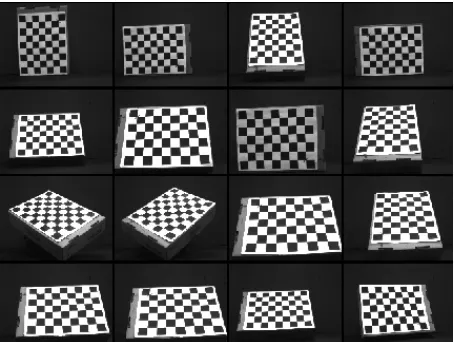
In camera modeling, one can employ a set of mathe- matical equations with the camera parameters being the main variables. The two cameras are calibrated using a 2D Plane based scheme, using a grid with check board pattern of 29 × 29 mm. The calibration can be done through one of two implementations, either moving the imagers while fixing the pattern or moving the pattern while fixing the imagers. In this study the second option is used.

Figure 1 displays the way that the calibration pattern is manipulated in space, from the left camera perspective. The higher the number of images that are taken for the different orientations, the higher the calibration accuracy. 32 images are captured for the calibration step; 16 im-ages from the right camera and 16 imim-ages from the left camera.

The calibration is done using approach developed by Jean [26]. The calibration results in the camera intrinsic and extrinsic parameters. The intrinsic parameters define the internal geometric and optical characteristics of the camera mainly; its Focal length (fc), horizontal and

verti-cal foverti-cal lengths fc(1), fc(2). The fc(2)/fc(1) is called the

aspect ratio . In the proposed camera system, the aspect ratio is set to about one because the camera pixels are

square. Other intrinsic factors include the Principalpoint (cc) and the skew coefficient (alpha_c), which defines the angle between the x and y axes. In this case, the coef- ficient is zero because of the square pixels used. Addi- tionally, the distortions (kc) are computed to describe the

image distortion coefficients including the radial and tangential distortions. In regard to the extrinsic parame- ters that describe the camera position and orientation with respect to the calibration pattern, they are repre- sented through two matrices; a rotation matrix R and a translational matrix T. These two matrices are used to uniquely identify the transformations between the un- known camera reference frame and the known world reference frame [27]. The extrinsic parameters depend on the camera pose/orientation and unlike the intrinsic pa- rameters, their values change once the camera pose is changed.

The calibration resulted in a pixel error around 0.21 pixels in the x-direction and around 0.45 pixels in the y-direction. The calibration error in mm units based on pixel pitch relation is found in tabulated in Table 1.

3.2. Correspondence Analysis

The traditional Sum of Square Difference or SSD algo-rithm employs a window around each pixel to search for close resemblance in the other perspective image. The comparison of the blocks is done using Equation (1);

   

, ,

T xy

SSD



where I(x,y) is pixel intensity in the first image (left im-age), and IT(x,y) is from the second image (right image).

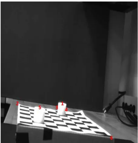
The block from the second window that has the smallest value of SSD as compared with others, is chosen as the window that closely resembles the block from the first image. The center of this block is then chosen as the cor-responding point of the pixel from the first image. The SSD algorithm based on intensity comparison has been tested using images shown in Figures 2(a)-(b), with a window size of 3 × 3 pixels. With six points selected for the comparison as shown in Figure 3, the resulted accu-racy is tabulated in Table 2. The SSD algorithm shows good results, however following challenges are identified; firstly, the code searches all pixels for correspondence which is not ideal because not all the same pixels exist in

Table 1. Error in calibration in mm units.

Image Size in mm units

Image size in pixels

Error in pixels

Error in mm units

x-direction

(Horizontal) 150 mm 640 pixels 0.21 pixels 0.05 mm y-direction

(Vertical) 110 mm 480 pixels 0.45 pixels 0.1 mm

(a) (b)

Figure 2. (a) Right image to test SSD algorithm; (b) Left image to test SSD algorithm.

Figure 3. Testing selection points in left image.

both images that might result in a false positive [28]. The SSD searches all the pixels in the right image 640 × 480 pixels, leading to long processing time for each corre-sponding pixel, which is found to be around 2.55 seconds for a machine that runs a core i7 CPU 2.67 GHZ, RAM 4 GB.

Figures 4(a) and (b) show two outputs from the tradi- tional SSD algorithm; one considered as the correct matching as in Figure 4(a), a while the other is a false matching case in Figure 4(b). Where the x-axis is the y coordinate of right image and y-axis is the minimum SSD. To minimize the high number of incorrect matching, a modified SSD algorithm is developed and further dis- cussed in Section 3.3.

3.3. Modified SSD Algorithm

Table 2. SSD test results.

Points coordinate in left image

Manually estimated position in right image

Calculated coordinate using SSD algorithm Points tag

X Y X Y X Y

Comments

1 357 300 357 408 357 411 Good correlation

2 387 108 387 220 387 223 Good correlation

3 375 285 375 393 375 391 Good correlation

4 375 315 375 423 375 417 Good correlation

5 382 203 382 246 382 368 False correlation

6 430 542 Does not exist in right image 430 265 False correlation

(a) (b)

Figure 4. (a) Good correlation related to point tag No. 3; (b) False correlation related to point tag No. 5.

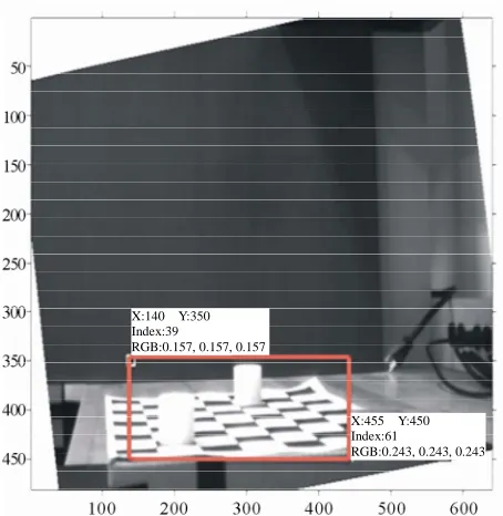
processing time. First change is done by implementing a specific Field of View for the search, by recognizing and establishing the region of interest within each image where the value-added information (objects) exists. In Figure 5, the new ROI is highlighted with a red border.

X:140 Y:350 Index:39

RGB:0.157, 0.157, 0.157

X:455 Y:450 Index:61

RGB:0.243, 0.243, 0.243 Second change is done by guiding the SSD algorithm

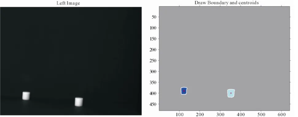
to search for detected objects’ Centroids. This modifica-tion can be implemented by threshold the image thusly removing the background (non-value added) information, in addition to filtering the resulted binary image to fur-ther remove data noise. Also, a combination of morpho-logical operations namely; erosion and dilation are done to help define the detected objects’ boundaries. Finally, the centroid can be readily detected as in Figure 6.

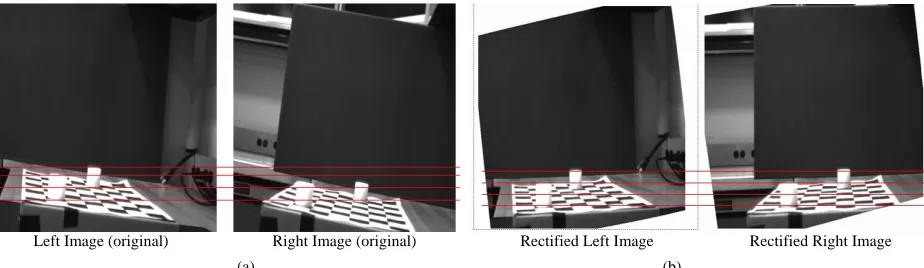
The third modification to the traditional SSD is done through a Rectification step. The rectification process determines a transformation of each image plane such that the pairs of conjugate epipolar lines become collin-ear and parallel to one of the image axes.

The distinct advantage of rectification is that

Figure 6. (a) Left image; (b) Objects’ boundaries and centroids.

search need only to consider the horizontal lines of the rectified images, reducing the search domain from 2D to 1D. The calibration step should be done before the recti- fication because the internal parameters should be known in this stage. The rectification [29] defines new Perspec- tive Projection Matrix PPM by rotating the old ones around their optical centers until the focal planes become coplanar, thereby containing the baseline. This ensures that the epipoles are at infinity; hence, epipolar lines are parallel. To have horizontal epipolar lines, the baseline must be parallel to the new x-axis of both cameras. In addition, to have a proper rectification, conjugate points must have the same vertical coordinate. The Perspective Projection Matrix PPM is found through the equation (2) below.





. \

PPMKK R T (2)

where, R is the rotational matrix, T is the translational matrix which found as extrinsic parameters in calibration step.

The camera matrix KK contains intrinsic parameters which found in calibration step.

 

 

 

 

 

1 _ 1

0 2

0 0

c c

c

f alpha c f cc

KK f cc

       1 2 1    (3)

The result of rectification step is found in Figures 7(a) and (b).

The results from the modified SSD code are in Table 3 showing good results in term of accuracy and resource efficiency. The error values are around 1.49 pixels in the x-direction and 2.72 pixels in the y-direction.

3.4. Triangulation

This section discusses the Integration of the modified

SSD algorithm along with the triangulation step. The triangulation is done in a passive mode to allow for more flexibility and robustness in terms of ambient lighting. Furthermore, the triangulation follows a linear square solution approach reported in [26], which is usefully summarized in following equations; suppose the coordi-nates for first cylinder in the right camera reference frame as; R R R R X P Y Z          

 (4)

And the coordinates for first cylinder in the left camera reference frame as;

L L L L X P Y Z          

 (5)

After the calibration, the extrinsic parameters like ro-tation matrix and translational matrix are known. Then the relation between PRand PL is;

L R

P  R P T (6)

Also, the projective of the two points pl and pron the

image plane is their perspective projection. Retrieving the PL and PR from the coordinates of the pl and pr results

in; 1 R R r R R x P p Z      _{  }    

y (7)

1 L L l L L x P p Z      _{  }    

Left Image (original) Right Image (original) Rectified Left Image Rectified Right Image (a) (b)

Figure 7. (a) Right and left image before rectification step; (b) Right and left image after rectification step.

Table 3. Results of modified SSD.

Actual Centroids for Two Cylinders Centroids using Modified SSD Algorithm The Maximum Error in Pixels

Left Image (389.9,123.7) (400.7, 354.0)

(390,124)

(401,354) 0.28

Right Image (388.1, 231.6) (399.5, 442.7)

(390,231)

(401,440) 1.49 in x-direction and 2.72 in y-direction Elapsed time 0.97 seconds. 0.02 seconds

By instituting these relations to the following Equation (9); results in Equation (10); upon re-arrangement be- comes Equation (11)

L R

P RP T (9)

L l R r

Z  P Z  R p T (10)

Rearrange the previous equation to:





r l L Z

R p p T

Z  

  _{ }

  (11) where, A  





 

R T T

L Z

A A A T

Z



    

  (12)

where,   Rpr With the final equation re-arranged

and written as (13) with < > representing a standard sca-lar product operator.

2 2 2 2 , , , , l l R l l

p T p p T

Z p p        l  (13)

where, , this is the x and y

coor-dinates of all objects Centroids in the left image and

, this is the corresponding points

found through modified SSD algorithm. 1 2 1 2 l x x p y y           1 2 1 2 x x y y           r p 

4. Results

The flow chart illustrated in Figure 8 displays the steps

followed when the proposed SSD algorithm is imple-mented.

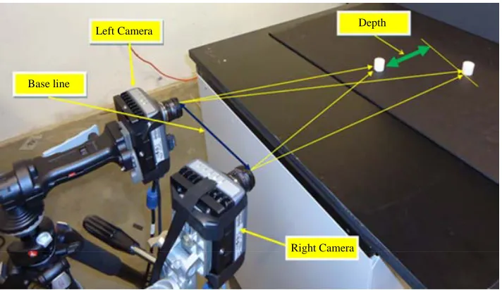
To test the stereo vision implementation with modified SSD algorithm, two experiments are done. The first ex-periment setup is shown in Figure 9, where two cylin-ders are placed in front of the left and the right cameras while their depths are calculated.

The optimal baseline for this experiment is around 20 cm, the close cylinder is placed around 90 cm from the cameras’ plane with the experiment repeated 7 times with new cylinder location for each time. The results are tabulated in Table 4, showing good agreement between the actual and the reported depths; the average depth er-ror is found to be around 1.2 mm while the maximum error in depth is around 2.9 mm.

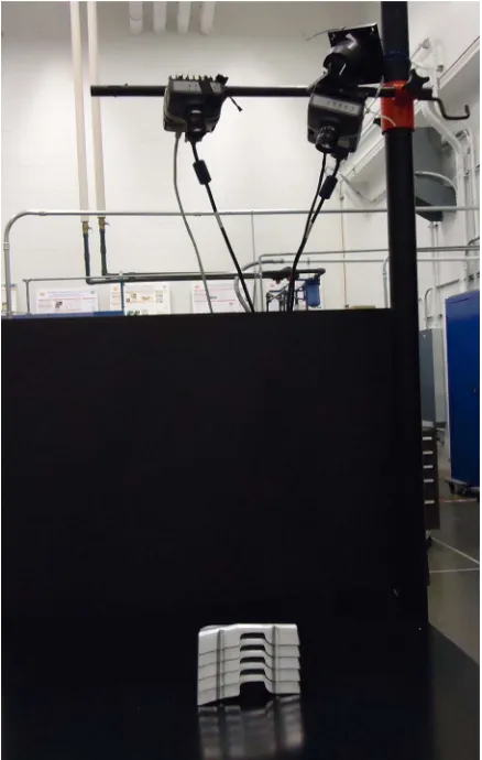
The second experiment is an implementation of an autonomous pick and place exercise. For this exercise, the goal is to compute the distance between the robotic gripper and the targeted objects. This is done by detect-ing the pick-up location for each object while compardetect-ing it to a ground reference so that the system can calculate the height of each acquisition. Additionally the targeted objects are arranged in a stack configuration that resem-bles real-life scenarios. The proposed setup calculates the depths to enable the gripper to accurately adjust for each object height and depth. Two CCD detectors are placed in a stereo-vision configuration while the gripper is placed (reference location) to be in the midpoint between the two detectors, on same base line. This setup is illus-trated in Figure 10.

Left Image Right Image Calibration Procedure

Rectification Procedure

Rectified Left Image

Rectified Right Image

Object Recognition

Calculate Left Centroids

Finding Corresponding Procedure

(SSD)

Calculate Right Centroids

Triangulation Procedure

Depth

Left Camera Right Camera

Figure 8. Flow chart to find triangulation using modified SSD algorithm.

Left Camera

Base line

Depth

Right Camera

Figure 9. Triangulation based on stereo vision.

Table 4. Triangulation results with baseline equal 20 cm.

Case No. Actual Depth in cm unit Calculated Depth in cm unit Depth Error in cm Percentage Error (%)

Case 1 10.00 10.10 0.1 1.00

Case 2 6.50 6.43 0.07 1.08

Case 3 19.00 18.83 0.17 0.89

Case 4 15.50 15.43 0.07 0.45

Case 5 12.50 12.37 0.13 1.04

Case 6 3.50 3.21 0.29 8.29

Case 7 24.00 23.96 0.04 0.17

location; the rectification results are further displayed in Figures 11 and 12.

The detected objects’ boundaries and their Centroids detection are modified to pinpoint two points; the pickup location and the reference ground point. Having these two locations identified, enable the code to compute the distances which are then sent to the gripper for actuation. This exercise is repeated six times using different num- ber of objects stacked on top of each other. Figure 13 shows the objects’ boundaries and the pick up location detection identified.

Figure 10. Triangulation based on stereo vision (Second experiment).

(a) (b)

Figure 11. Before rectification: (a) Left image; (b) Right image.

(a) (b)

Figure 12. After rectification: (a) Left image; (b) Right im-age.

Rectified Left Image Draw Boundary and centroids

Pick up location

(a) (b)

Figure 13. (a) Rectified left image; (b) Objects’ boundaries and pickup location.

5. Conclusion

The presented study proposed a modified, efficient SSD algorithm that can be used within the context of ste- reo-triangulation for autonomous pick and place. The suggested modifications were in two folds; reducing the search domain by establishing a ROI for the value-added data and through a rectification step that is done to re- duce the 2D search domain into 1D. The second fold relied on the use of detected objects’ centroids rather than their pixels’ intensities. Thusly is improving the code robustness against any changes in the surroundings’ illumination. The developed code results in better accu- racy and repeatability, without any false positives at faster processing times. An autonomous pick and place exercise is also demonstrated using the developed algo- rithm, future work includes further refinement to the SSD code to improve its processing efficiency and robustness.

REFERENCES

[1] C. Tyler, “Binocular Vision,” Foundations of Clinical Ophthalmology, Vol. 2, Chapter 24, 1982.

http://www.ski.org/CWTyler_lab/CWTyler/TylerPDFs/T yler_BinocVisionDuanes2004.pdf

[2] G. DeAngelis, B. Cumming and W. Newsome, “Cortical Area MT and the Perception of Stereoscopic Depth,” Jour- nal Nature, Vol. 394, 1998, pp. 677-680.

[3] R. Kletter, K. Schluns and A. Koschan, “Three-Dimen- sional Data from Images,” 2nd Edition, Springer-Verlag Singapore Pte. Ltd., Singapore, 1998.

High-Accuracy 3D Machine Vision Metrology Using of the Shelf TV Cameras and Lenses,” IEEE Journal of Ro- botics and Automation, Vol. 3, No. 4, 1987, pp. 323-344. doi:10.1109/JRA.1987.1087109

[5] O. Faugeras, “Three-Dimensional Computer Vision: A Geo- metric Viewpoint,” MIT Press, Cambridge, 1993.

[6] Z. Zhang, “A Flexible New Technique for Camera Cali- bration,” IEEE Transactions Pattern Analysis and Ma- chine Intelligence, Vol. 22, No. 11, 2000, pp. 1330-1334. doi:10.1109/34.888718

[7] Z. Zhang, “Camera Calibration with One Dimensional Ob- jects,” IEEE Transactions Pattern Analysis and Machine Intelligence, Vol. 26, No. 7, 2004, pp. 892-899.

[8] S. T. Barnard and M. A. Fischler, “Stereo Vision,” Ency-clopedia of Artificial Intelligence, John Wiley, New York, 1987, pp. 1083-1090.

[9] T. Kanade and M. Okutomi, “A Stereo Matching Algo-rithm with Adaptive Window: Theory and Experiment,” IEEE Transactions on Pattern Analysis and Machine In-telligence, Vol. 16, No. 9, 1994, pp. 869-881.

doi:10.1109/34.310690

[10] H. Moravec, “Towards Automatic Visual Obstacle Avoid- ance,” Proceedings of the 5th International Joint Conference on Artificial Intelligence, Cambridge, 22-25 August 1977, p. 584.

[11] P. Premaratne and F. Safaei, “Stereo Correspondence Us- ing Moment Invariants,” Communications in Computer and Information Science, Vol. 15, No. 12, 2008, pp. 447-454.

doi:10.1007/978-3-540-85930-7_57

[12] M. Pilu, “A Direct Method for Stereo Correspondence Based on Singular Value Decomposition,” Proceedings of

1997 IEEE Computer Society Conference on Computer

Vision and Pattern Recognition, San Juan, 17-19 June 1997, pp. 261-266.

[13] G. L. Scott and H. C. Longuet-Higgins, “An Algorithm for Associating the Features for Two Patterns,” Proceedings of Royal Society London, Vol. B244, No. 1309, 1991, pp. 21-26. doi:10.1098/rspb.1991.0045

[14] M. Hebert, “Active and Passive Range Sensing for Ro- botics,” Proceedings of the 2000 IEEE International Con-ference on Robotics & Automation, San Francisco, 24-28 April 2000, pp. 102-110.

[15] D. Jingting, L. Jilin, Z. Wenhui, Y. Haibin, W. Yanchang and G. Xiaojin, “Real-time Stereo Vision System Using Adaptive Weight Cost Aggregation Approach,” EURASIP Journal on Image and Video Processing, Vol. 2011, No. 20, 2011, pp. 1- 19. doi:10.1186/1687-5281-2011-20

[16] P. Azad, T. Asfour and R. Dillmann, “Accurate Shape-Based 6-DoF Pose Estimation of Single-Colored Objects,” The 2009 IEEE/RSJ International Conference on Intelligent Ro-

bots and Systems, St. Louis, 11-15 October 2009, pp. 2690-2695.

[17] M. Zaheer and B. Mertsching, “Pre-Attentive Detection of Depth Saliency Using Stereo Vision,” 2010 IEEE 39thAp- plied Imagery Pattern Recognition Workshop AIPR, 2010, pp. 1-7.

[18] W. Iversen, “Vision-Guided Robotics: In Search of the Holy Grail,” Automation World, 2006, pp. 28-31. http://www.automationworld.com/feature-1878

[19] A. Pochyly, T. Kubela, M. and P. Cihak, “Robotic Vision for Bin-Picking Applications of Various Objects,” 2010 41st International Symposium on and 20106th German Conference on Robotics, Munich, 7-9 June 2010, pp. 1-5.

[20] B. Kazunori, W. Fumikazu, K. Ichiro and K. Hidetoshi, “Industrial Intelligent Robot,” FANUC Technology Review Journal, Vol. 16, No. 2, 2003, pp. 35-41.

[21] J. Porrill, S. B. Pollard, T. P. Pridmore, J. B. Bowen, et al., “TINA: A 3D Vision System for Pick and Place,” Image and Vision Computing, Vol. 6, No. 2, 1988, pp. 65-72.

[22] T. Kotthäuser and F. Georg, “Vision-Based Autonomous Ro- bot Control for Pick and Place Operations,” 2009 IEEE/ ASME International Conference on Advanced Intelligent Mechatron- ics Suntec Convention and Exhibition Center, Singapore, 14- 17 July 2009, pp. 1851-1855.

[23] K. Rahardja and A. Kosaka, “Vision-Based Bin-Picking: Recognition and Localization of Multiple Complex Objects Using Simple Visual Cues,” Proceedings of IEEE/RSJ In- ternational Conference on Intelligent Robots and Systems, 4-8 October 1996, pp. 1448-1457.

[24] B. Martin, B. Bachler and S. Stefan, “Vision Guided Bin Pick- ing and Mounting in a Flexible Assembly Cell,” Thirteenth In- ternational Conference on Industrial and Engineering Appli- cation of Artificial Intelligence and Expert Systems, New Or- leans, 19-20 June 2000, pp. 255-321.

[25] H. Chengalvarayan, P. Murugesapandian, N. Ramachandran and S. Yaacob, “Stereo Vision System for A Bin Picking Adept Robot,” Malaysian Journal of Computer Science, Vol. 20, No. 1, 2007, pp. 91-98.

[26] J. Bouguet, “Camera Calibration Toolbox for Matlab,” 2010. http://www.vision.caltech.edu/bouguetj/calib_doc/

[27] E. Trucco and A. Verri, “Introductory Techniques for 3-D Computer Vision,” Prentice-Hall, 1998.

[28] N. Ayache and P. Sander, “Artificial Vision for Mobile Robots: Stereo Vision and Multisensory Perception,” MIT Press, Cambridge, 1991.

[29] A. Fusiello, E. Trucco and A. Verri, “A Compact Algori- thm for Rectification of Stereo Pairs,” Machine Vision and Applications, Vol. 12, No.1, 2000, pp. 16-22.