Numerical Solution of the Fredholme-Volterra Integral
Equation by the Sinc Function
Ali Salimi Shamloo, Sanam Shahkar, Alieh Madadi
Department of Mathematics, Islamic Azad University, Shabestar Branch, Shabestar, Iran Email: [email protected], {sanam_shahkar, a_madadi6223}@yahoo.com
Received March 4,2012; revised April 9, 2012; accepted April 17,2012
ABSTRACT
In this paper, we use the Sinc Function to solve the Fredholme-Volterra Integral Equations. By using collocation method we estimate a solution for Fredholme-Volterra Integral Equations. Finally convergence of this method will be discussed and efficiency of this method is shown by some examples. Numerical examples show that the approximate solutions have a good degree of accuracy.
Keywords: Fredholme-Volterra Integral Equation; Sinc Function; Collocation Method
1. Introduction
The sinc function form for the interpolating pointIn recent years, many different methods have been used to approximate the solution of the Fredholme-Volterra In-tegral Equations, such as [1,2]. In this paper, we first present the Sinc Function and their properties. Then we consider the Fredholme-Volterra Integral Equation types in the forms
1
, d 2
,b b
a a
u x f x
k x t u t t
k x t u t dt
(1.1) where , and f(x) are known functions, but u(x) is an unknown function. Then we use the Sinc Function and convert the problem to a system of linear equations.
1 ,
k x t k2
x t,2. Sinc Function Properties
The sinc function properties are discussed thoroughly in [3-10]. The sinc function is defined on the real line by
sin
π ,sin π
1, 0
x x
c x x
x
0, (2.1)
For , and The translated sinc functions with evenly spaced nodes are given by
0
h k 0, 1, 2, ,
, sin
π
sin
, ,
π
1, ,
x jh
S j h x c
h
x jh h
x jh x jh
h
x jh
(2.2)
k
x kh is given by
, 0 1, ,0, .
jk
k j
S j h kh
k j
(2.3)
Let
1
0
sin π
1
d ,
2 π
k j kj
t t t
(2.4)If a function u x
is defined on the real axis, thenfor h > 0 the series
,
sinj
,
x jh
c u h x u jh c
h
(2.5)called whittaker cardinal expansion of , whenever this series converges. The properties of the whittaker cardinal expansion have been extensively studied in [8].
u
These properties are derived in the infinite stripe D of the complex w- plane, where for d0,
, Im , 0
D w C w d d
Approximations can be constructed for infinite, semi- infinite and finite intervals. To construct approximations on the interval [a,b], which is used in this paper, the eye- shaped domain in the z-plane.
π
: arg ,
2
E
z a
D z x iy d
b z
Is mapped conformably onto the infinite strip D via
, 1
exp
1 exp
a b w
z a
w z Ln z w
b z w
The basis functions on [a,b] are taken to be composite translated sinc functions,
, sin
x jhs k h o x c
h
, (2.6) Thus we may define the inverse images of the real line and of evenly spaced nodes
jh j as
t DE:
a b, t ,
and
1 , 0, 1, 2,
1
kh
k kh
a be
x kh k
e
(2.7)
We consider the following definitions and theorems in [8-10].
Definition 2.1:
Let L
DE be the set of all analytic functions, forwhich there exists a constant, C, such that
2 , ,01 E
z
u z c z D
z
1
(2.8)
Theorem 2.1:
Let uL
DE , let N be appositive integer, and let hbe
1 2
πd h
N
(2.9)
Then there exists positive constant C1, independent of
N, such that
π 12 1
sup N j , d N
z j N
u z u z S j h o z C e
(2.10)Proof: See [8,9]. Theorem 2.2:
Let uL
DE , Let N be a positive integer and let h be selected by the relation (2.9) then there exist posi-tive constant C2, independent of N, such that
π 12 2
d N j d N
Z
j N j
u z
u z h C e
z
(2.11)and also for 0 π,0 1,let 1
kj
d
3
C
be defined as in (2.4) then there exists a constant, which is inde-pendent of N, such that
π 1
1 2
3
d k
z N
d N kj
J N a
u zk
u t t h C e
zk
(2.12)Proof: See [8].
3. The Sinc Collocation Method
The solution of linear Fredholm-Volterra integral Equa-tion (1.1) is approximated by the following linear com-bination of the sinc functions and auxiliary functions:
N
j j
,
,j N
u x u x x x a b
(3.1)where
,
, , 1, ,
,
a j
b
w x j N
x s j h o x j N N
w x j N
1,
(3.2)
where the basis functions wa
x w, b
x defined by
1
, 1a
w x
x
(3.3)
, 1b
x
w x
x
(3.4)
xx e
(3.5) We denote a a and b b then basis function
must satisfy the following conditions:
lim 1, lim 0,
a a a b
x w x x w x (3.6)
lim 0, lim 1
b
b b
x w x xbw x
(3.7)Obviously by using Equations (2.3) and (3.1) we have
a -N,
b Nu u u u .
Lemma 3.1:
Eu x L D , let N be a positive integer and
π
12h d N , Then (see Equation (3.8)), where j
xis defined in (2.14) and C4 is a positive constant, inde-pendent of N.
Proof: See [9]. Lemma 3.2:
For u x
defined in (3.1), let
1 , 2
j E j E
k k
L D L D
,
and h be selected from (2.9) then (see Equation(3.9))
1
π 124 1
sup ( N , d N
N a N j N b N
x j N
u x u x w x u x S j h o x u x w x C e
(3.8)
1 ( 1) 2
1 2
1
1 ( 1) 2 1 ( 1) 2
1
, ,
, d , d
, , , ,
( ) ( )
k
x
b N
j k j
N kj a j
j N
a a j j
N N
j k j j k j
j kj N kj b j
j N j j j N j j
k x t k x t
k x t u t t k x t u t t hu x w t
t t
k x t k x t k x t k x t
h u x hu x w t
t t t t
(3.9)Now let u x
be the exact solution (1.1) that isap-proximated by following expansion.
N
,
, , 2n j j j N
u x u x x a b n N
1 (3.10)Upon replacing u x
in the Fredholm-Volterrainte-gral Equation (1.1) un
x , applying Lemma 3.1 andLemma 3.2, setting sinc collocation points xk and
Then, considering (0)
kj
(0
jk
)
we obtain the following system
1
1 ( 1) 2 (0) 1 ( 1) 2
1 2 ( 1) 1 , , , , , N N k j
k j k j k j
N a k kj a j kj kj
j N j j j N j j
N
k j k j
N b k kj b j
j N j j
k x t
k x t k x t k x t
u w x h w t h u
t t t t
k x t k x t
u w x h w t
t t , j
k , , ,f x k N N
(3.11)
We write the above system of equations in the matrix forms:
( 2) 1
, where n n 2 1
n
TU P T A B C U n N
(3.12)
where
1 1 2
1 ( 1) 2
, , , , , , , N
N j N j
a N Nj a j a N
j N j j
T N
N j N j
Nj a j
j N j j
k x t k x t
A w x h w t w x
t t
k x t
k x t
h w t
t t
(3.13)
1 1(0) , 2 , ,
, , 1, , 1
k j k j
kj kj
j j
k x t
k x t
B h
t t
k N N j N N
T
(3.14)
1 ( 1) 2
1 ( 1) 2
, ,
( ), , ( )
, ,
j
N
N j N j
b N Nj a j b N
j N j j
T N
N j N j
N b j
j N j j
k x t k x t
C w x h w t w x
t t
k x t k x t
h w t
t t
, (3.15)
, 1
, ,
1
)T
N N N N
p f x f x f x f x (3.16)
, 1, , 1,
T N N N N
U u u u u
j
u xim
,
By solving the above system we obtain, (3.17)
0 ... 0 1 ... 0
a N b N
a N b N
w x w
w x w x
1 1 1 1 . . . . , . . . . .0 ... 1 0 ... 0
n u u
a N b N
a N b N
x
U I U I
w x w x
w x w x
. (3.18)
4. Convergence Analysis
Now we discuss the convergence each of sinc collocation the exact solution of the ation (1.1). For each N,
method. Suppose that u x
is Fredholme-Volterra integral Equwe can find uj which is our solution of the liner system
(3.12), also by using uj obtain the approximate
so-lution un
x , In order to derive a bound for |u(x) - un(x)|we need to es te the norm of the vector Tup, where
u is a vector defined
we
by tima
, ,
TN N
u u x u x here ( )
w u xj is the value of the exact solution of
inte-gral equation at the sinc points xj. Th for we need
the fo emma.
f ere llowing l
Lemma 4.1:
Let u(x) be the exact solution o the integral (1.1) and
Eu x L D let
π
12 1
, 2
,j E j E
k k
h d N and L D L D
for x
a b,N, such
, then there exists a constant C5 independ-ent of that
1 1
T
Theorem 4.1:
Let us consider all assumptions of Lemm
2 2
5 exp π
up C N d N (4.1) Proof: See [10].
a 3.1 and let
n x be the appr
u
ter
oximate solution of Fredholme-Vol- tion given by (3.3) then we have ra integral equa
12
126
sup exp π
x
n
u x u x CN d N
(4.2)
where C6 a constant independent of N, and T1 Proof:
Suppose n
x defined this following form:j
n
N,
j j N
x u x x
(4.3)
So we have
, , , , , a j bw x j N
x S j h o x
w x j N
, 1, , 1,
j N N
n
n
n
n
u x u x u x x x u x .4) By using Lemma 3.1, we obtain
(4
124
sup n exp π
x
u x x C d N
Obviously by using Equations (4.3) and (3.3) we have.
1 1 2 2 2 2 N N 1 N Nn n j j j j
j N j N
j j j
j N j N
x u x u x x u
u x u x E
(4.5)And we have from definition of the
x
j
We obtain
1 2 2 7 N j j N x C
(4.6)Now, by using Equations (4.5) and (4.6) we get That C7 a constant independent of N.
1 7
E C UU
nd lemma 4.1 w
(4.7) In this case by using the system (3.12) a
e obtain
1 1
U U T T U U T
1 1
2 2
5 exp π ,
C N d N
TU P
(4.8)
Now by using Equations (4.7) and (4.8) we get
12
12 (4.9)8 exp π
n n
B x u x CN d N
e ob-ta
Obviously by using Equations (4.9) and (4.2) w in
1 2 4 1 1 2 2 8 1 1 2 2 66 4 8
sup exp π
exp π
exp π
max , .
n x
u x u x C d N
C N d N
C N d N
C C C
5. Numerical Examples
In this section, we apply the sinc collocation method for solving Fredholm-Volterra integral equation example.
llowing Fredholm-Vol- nd with exact so-Example 5.1: Consider the fo
terra integral equation of the second ki lution u(x) = x.
0 0
d d
3 3
u x x
tx u t t
tx u t t1 4
2 x
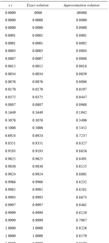
Table 3. Results for Example 1
Exact solution Approximation solution
We solved Example 5.1 for different of 1
, π ,
2
N and h N
And we consider the sinc grid points as:
N, N 1, , N 1, N
, s x x x xwhere
, , ,
1
k kh kh
a be
x k N N
e
The errors on the given points are denote by d
max
s j n j
E h u x u x
N j N
[image:5.595.309.539.99.613.2] (5.1) .
Table 1. Results for Example 1 (N = 5). x i Exact solution Approxima
Computational results are given in Tables 1-5
tion solution
0.0009 0.0009 0.0010
0.0036 0.0036 0.0045
0.0146 0.0146 0.0177
0.0568 0.
0.0568 0.0662
1970 0.1970 0.2175
0.5000 0.5000 0.5269
0.8030 0.9432
0.8030 0.9432
0.8082 0.9054
0.9854 0.9854 0.8836
0.9964 0.9991
0.9964 0.9991
0.8332 0.7733
Table 2. Results for Example 1 ). Ex ion Approximation solution
(N = 10
x i act solut
0.0000 0.0000 0.0001
0.0001 0.0001 0.0002
0.0004 0. 0.0010 0.
0004 0.0004
0.0010 0.0011
0026 0.0026 0.0029
0.0069 0.0069 0.0080
0.0185 0.0185 0.0223
0.0483 0.0483 0.0585
0.1206 0.1206 0.1419
0.2702 0.2702 0.3044
0.5000 0.5000 0.5381
0.7298 0.7298 0.7520
0.8794 0.8794 0.8634
0.9517 0.9517 0.8791
0.9815 0.9815 0.8465
0.9931 0.9931 0.8009
0.9974 0.9974 0.7850
0.9990 0.9990 0.8269
0.9996 0.9996 0.8753
0.9999 0.9999 0.8777
1.0000 1.0000 0.8443
(N = 15).
x i
0.0000 .0000 .00000
0.0000 0.0000 0.0000
0.0000
0.
0.0000 0.0000
0001 0.0001 0.0001
0.0001 0.0001 0.0002
0.0003 0.0003 0.0004
0.0007 0.0007 0.0008
0.0015 0.0015 0.0018
0.0034 0.0034 0.0039
0.0076 0.0076 0.0086
0.0170 0.0170 0.0197
0.0375 0.0375 0.0447
0.0807 0.0807 0.0968
0.1649 0.1649 0.1942
0.3076 0.3076 0.3496
0.5000 0.5000 0.5452
0.6924 0.6924 0.7237
0.8351 0.8351 0.8327
0.9193 0.9193 0.8656
0.9625 0.9625 0.8491
0.9830 0.9830 0.8155
0.9924 0.9924 0.8001
0.9966 0.9966 0.8232
0.9985 0.9985 0.8581
0.9993 0.9993 0.8673
0.9997 0.9997 0.8461
0.9999 0.9999 0.8129
0.9999 0.9999 0.7987
1.0000 1.0000 0.8226
1.0000 1.0000 0.8579
1.0000 1.0000 0.8672
nsider the following Fredholm- Volterra integral equation of the second kind with exact so
Example 5.2: we co
lution
2 x
.
u x
0 0
3 d d
12 6 4 2 2
x x x x t
x xt u t t u t t
1
3 4 x
u
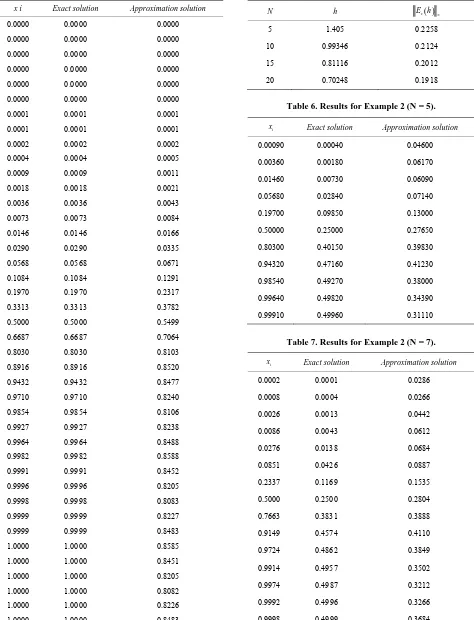
[image:5.595.59.284.466.735.2]Tab sults for Examp Table 4. Results for Example 1 (N = 20).
x i Exact solution Approximation solution
0.0000 0.0000 0.0000
0.0000 0.0000 0.0000
0.0000
0.
0.0000 0.0000 0.0000
0.0000 0.0000
0000 0.0000 0.0000
0.0000 0.0000 0.0000
0.0001 0.0001 0.0001
0.0001 0.0001 0.0001
0.0002 0.0002 0.0002
0.0004 0.0004 0.0005
0.0009 0.0009 0.0011
0.0018 0.0018 0.0021
0.0036 0.0036 0.0043
0.0073 0.0073 0.0084
0.0146 0.0146 0.0166
0.0290 0.0290 0.0335
0.0568 0.0568 0.0671
0.1084 0.1084 0.1291
0.1970 0.1970 0.2317
0.3313 0.3313 0.3782
0.5000 0.5000 0.5499
0.6687 0.6687 0.7064
0.8030 0.8030 0.8103
0.8916 0.8916 0.8520
0.9432 0.9432 0.8477
0.9710 0.9710 0.8240
0.9854 0.9854 0.8106
0.9927 0.9927 0.8238
0.9964 0.9964 0.8488
0.9982 0.9982 0.8588
0.9991 0.9991 0.8452
0.9996 0.9996 0.8205
0.9998 0.9998 0.8083
0.9999 0.9999 0.8227
0.9999 0.9999 0.8483
1.0000 1.0000 0.8585
1.0000 1.0000 0.8451
1.0000 1.0000 0.8205
1.0000 1.0000 0.8082
1.0000 1.0000 0.8226
1.0000 1.0000 0.8483
le 5. Re le 1.
N h E hs
5 1.405 0.2258
10 0.99346 4
15 012
20 0.70248 0.1918
0.212
[image:6.595.62.536.101.721.2]0.81116 0.2
Table 6. Results for Example 2 (N = 5).
i
x Exact solution Approximation solution
0.00090 0.00040 0.04600
0.00360 0. 0.0617
0.01460
0.05680 0.
0.80300 0.40150 0.39830
0.99640 0.49820 0.34390
00180 0
0.00730 0.06090
02840 0.07140
0.19700 0.09850 0.13000
0.50000 0.25000 0.27650
0.94320 0.47160 0.41230
0.98540 0.49270 0.38000
0.99910 0.49960 0.31110
Table 7. Results for Example 2 (N = 7).
i
x Exact solution Approximation solution
0.0002 0.0001 0.0286
0.0008 0.0004 0.0266
0.0026
0.0086 0.
0.0276 0.0138 0.0684
0.0851 0.0426 0.0887
0.2337 0.1169 0.1535
0.5000 0.2500 0.2804
0.7663 0.3831 0.3888
0.9149 0.4574 0.4110
0.9724 0.4862 0.3849
0.9914 0.4957 0.3502
0.0013 0.0442
0043 0.0612
0.9974 0.4987 0.3212
0.9992 0.4996 0.3266
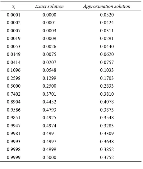
Table 8. Results for Example 2 (N = 9).
i
x Exact solution Approximation solution
0.0001 0.0000 0.0520
0.0002 0.0001 0.0424
0.0007 0.0003 0.0311
0.0019 0.00
0.0009 0.0291
53 0.0026 0.0440
0.0149 0. 0.0414
0075 0.0207
0.0620 0.0757
0.1096 0.0548 0.1033
0.2598 0.1299 0.1703
0.5000 0. 0.7402
2500 0.3701
0.2833 0.3810
0.8904 0.4452 0.4078
0.9586 0.4793 0.3873
0.9851 0. 0.9947
4925 0.4974
0.3548 0.3283
0.9981 0.4991 0.3309
0.9993 0.4997 0.3638
0.9998 0. 0.9999
4999 0.5000
0.3852 0.3752
Table 9. Results for Example 2.
N h E hs
5 1.4050 0.1885
7 1.1874
9 1. 17 0.
0. 0.1586
0.1775
0472 0.1690
7619 0.1608
20 7025
30 0.5736 0.1540
REFERENCES
[1] azzadeh tfi, “Collocation Method for
Fredholm-Vol with Weakly Ker-
S. Fay and M. Lo
terra Integtral Equations
nels,” International Journal of Mathematical Modelling & Computations, Vol. 1, 2011, pp. 59-58
[2] A. Shahsavaran, “Numerical Solution of Nonlinear Fred- holm-Volterra Integtral Equations via Piecewise Constant Function by Collocation Method,” American Journal of Computational Mathematics, Vol. 1, No. 2, 2011, pp. 134- 138.
[3] F. Stenger, “Numerical Methods Based on the Whittaker Cardinal or Sinc Functions,” SIAM Review, Vol. 23, No. 2, 1981, pp. 165-224.
[4] J. Lund, “Symmetrization of the Sinc-Galerkin Method for Boundary Value Problems,” Mathematics of Compu- tation, Vol. 47, No. 176, 1986, pp. 571-588.
[5] B. Bialecki, “Sinc-Collocation Methods for Two-Point Boundary Value Problems,” IMA Journal of Numerical Analysis, Vol. 11, No. 3, 1991, pp. 357-375.
doi:10.1093/imanum/11.3.357
[6] N. Eggert, M. Jarrat and J. Lund, “Sinc Function Compu- tation of the Eigenvalues of Sturm—Liouville Problems,” Journal of Computational Physics, Vol. 69, No. 1, 1987, pp. 209-229. doi:10.1016/0021-9991(87)90163-X [7] M. A. Abdou and O. L. Mustafa, “Fredholm-Volterra Inte-
gral Equation in the Contact Problem,” Applied Mathe- matics and Computation, Vol. 138, No. 2-3, 2002, pp. 1- 17.
[8] J. Land and K. Bowers, “Sinc Methods for Quadrature and Differential Equations,” Society for Industrial and Applied Mathematics, Philadelphia, 1992.
[9] F. Stenger, “Numerical Methods Based on Sinc and Ana- lytic Function,” Springer-Verlag, New York, 1993. [10] J. Rashidinia and M. Zarebnia, “Solution of a Volterra
[image:7.595.58.288.99.371.2]