GeoMatch:Efficient Large Scale Map Matching on Apache Spark

GeoMatch: Efficient Large-Scale Map Matching on Apache Spark

Ayman Zeidan

Department of Computer Science, CUNY Graduate Center

New York, NY USA [email protected]

Eemil Lagerspetz

Department of Computer Science, University of Helsinki

Helsinki Finland [email protected]

Kai Zhao

Robinson College of Business, Georgia State University,

Atlanta Georgia, USA [email protected]

Petteri Nurmi University of Helsinki and

Lancaster University Helsinki, Finland

Lancaster, UK [email protected]

Sasu Tarkoma

Department of Computer Science, University of Helsinki

Helsinki Finland [email protected]

Huy T. Vo

Department of Computer Science, CUNY City College New York, NY, USA [email protected]

Abstract—We contribute by developing GeoMatch as a novel, scalable, and efficient big-data pipeline for large-scale map matching on Apache Spark. GeoMatch improves ex-isting spatial big data solutions by utilizing a novel spatial partitioning scheme inspired by Hilbert space-filling curves. Thanks to the partitioning scheme, GeoMatch can effectively balance operations across different processing units and achieve significant performance gains. We demonstrate the effectiveness of GeoMatch through rigorous and extensive benchmarks that consider data sets containing large-scale urban spatial data sets ranging from166,253 to 3.78 billion location measurements. Our results show over 17-fold performance improvements compared to previous works while achieving better processing accuracy than current solutions (97.48%).

Keywords-Big Data, Spatial Data Analysis, Spatial Partition-ing, Performance, Query ProcessPartition-ing, Spark

I. INTRODUCTION

The availability of urban location data has grown ex-ponentially thanks to the widespread and penetration of location technologies to cars, buses, trains, and other means of transportation. Indeed, data sets containing millions or even billions of location measurements collected from taxi-cabs1_{, buses}2_{, and fleet management are becoming available.}

This growth of spatial data is opening up unprecedented opportunities to analyze and understand mobility and how it relates to urban infrastructure. For example, research has shown how this data can be used to characterize urban mobility patterns, detect transportation bottlenecks, and to optimize transportation infrastructure [1]–[4]. Besides aca-demic interest, the increased amount of spatial data also has significant commercial potential, with the market value of spatial big data industry expected to rise to $440 by2020[5].

AUTHORS’ COPY — PREPRINT. To be published in Proceedings of the 2018 IEEE International Conference on Big Data, Seattle, 2018.

1_{NYC Taxi data set contains over 3.7 billion points.} 2_{NYC Bus data set contains over 216 million points.}

New York City TPEP Point Distribution

102

103

104

105

106

107

Nu

mb

er

o

f

G

PS

Po

in

ts

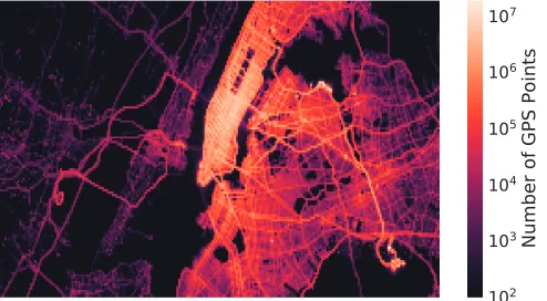
Figure 1: Sample distribution for a data set containing taxi trajectories collected from NYC (logarithmic scale).

slow or even failing entirely. The main reason for the poor performance is the sub-optimal partitioning of measurements as current solutions mainly rely on a random sampling of the data and excessive caching. This results in a partitioning that is sensitive to how the measurements are organized into files and the spatial distribution of measurements. Figure 1 illustrates this problem by showing the spatial distribution of measurements for one of the data sets considered in our experiments. Since the majority of measurements are concentrated along few small areas, the resulting partitioning is unbalanced, and a small number of cluster nodes perform most of the processing instead of having evenly distributed processing across the nodes.

To improve performance of large-scale map matching, we contribute GeoMatch, a novel distributed map match-ing extension for Spark. GeoMatch natively and efficiently matches GPS points to road segments. It eliminates the need for sampling by creating a locality preserving partitioning that builds on Hilbert space-filling curves and their use for spatial indexing [10]. Once the index has been built, Geo-Match uses an efficient and intuitive load balancing scheme to evenly distribute the parts of the index between available computing cores. As we experimentally demonstrate, these steps allow GeoMatch to achieve significant performance improvements compared to previous frameworks. GeoMatch will be released as open-source in 20183_.

We evaluate GeoMatch through rigorous and extensive map matching benchmarks using three data sets that range from 166_,253 _to 3_.78 _{billion measurements. We compare}

GeoMatch against three popular Spark spatial extensions (LocationSpark, Magellan, and GeoSpark). The results of our experiments demonstrate that GeoMatch is capable of achieving up to 17_{folds faster runtime performance, more}

stable scalability, and precise spatial object support. More-over, for our largest dataset LocationSpark, Magellan, and GeoSpark struggle significantly due to the size of the data set achieving slow performance and even running out of memory. Finally, we demonstrate that the indexing scheme used by GeoMatch improves map matching performance by

9.12-fold and results in an overall accuracy of97.48%.

Summary of contributions:

1) An effective indexing technique based on Hilbert Space-filling curves that expedites spatial query processing in a distributed computing environment. The technique eliminates the need to sample either data set resulting in a partitioning scheme which reduces memory and computing requirements.

2) A quick and natural load balancing technique that helps in mitigating query skews – a problem that overloads some partitions while others are left underutilized. 3) A Spark-based map matching pipeline for processing

truly large spatial data sets. It is scalable and outperforms

3_{https://github.com/bdilab/GeoMatch}

other techniques in resource requirements and accuracy. It is 1.6x–17x faster than current works in large-scale map matching and achieves 97.48%accuracy and9.12x faster processing speed compared to exhaustive search. 4) A format-independent technique that is easy to integrate

with existing spatial data processing systems.

II. RELATEDWORK

Spatial big-data processing frameworks extend generic frameworks like Apache Hadoop or Apache Spark by in-cluding support for spatial data structures and operations.

Hadoop based frameworks focus on making MapReduce

tasks spatially aware. However, they inherit Hadoop’s fault-tolerance limitation and must write intermediate results to HDFS. Esri GIS Tools for Hadoop [11] is a set of Hive User Defined Functions that are mainly released as a util-ity to extend the functionalutil-ity of Esri’s ArcGIS mapping software to include support of Well-Known Text (WKT) files stored on Hadoop. Hadoop-GIS [12] is built on top of Hadoop and adopts a streaming approach. It extends Hive to offer support for spatial objects and operations and translate queries into spatially capable MapReduce tasks. SpatialHadoop [7] has fewer interactions with HDFS than Hadoop-GIS and its MapReduce tasks are more spatially aware since they operate on data as spatial objects from the start. SATO [13] is a generic solution for optimal spatial partitioning on MapReduce systems with the main objective of targeting the spatial partitioning problem which causes query skews. It can be used as a standalone program but it has been integrated into Hadoop-GIS.

Spark based frameworks rely on Spark’s Resilient

Dis-tributed data set (RDD). RDDs are the core technology of Spark which solved two major Hadoop drawbacks — the limited in-memory processing and the need to write intermediate results to disk to achieve fault-tolerance. Spa-tialSpark [14] offers two modes of operation; Broadcast spatial join which is ideal for use with one small data set and one large data set, and Partitioned spatial join which is ideal for two large data sets. Simba [15] allows spatial operations using Spark SQL or DataFrames and represents its data sets as tables. SQL queries are optimized using a Cost-Based Optimizer (CBO) in order to produce an optimal parallel execution plan. Simba, on the other hand, focuses on multidimensional queries by indexing each dimension separately ultimately increasing query’s complexity.

spatial queries using standard SQL or DataFrame. Magellan examines the user’s query and object types in order to build and optimize the query execution plan. GeoSpark [6] introduces SRDD (Spatial RDD), an extension of Spark’s RDD that allows users to execute spatial operations.

Hilbert Space-Filling Curve (HSFC)is a powerful spatial

data indexing and partitioning method. Spatial objects can be mapped to one or more HSFC indexes which in turn groups nearby objects (indexes) together. GeoSpark offers a HSFC partitioning scheme that decides on the best way to partition the data sets. In SATO, HSFC is recommended as a technique to obtain an approximate total ordering while preserving spatial locality. LocationSpark uses HSFC to enhance kNN join queries an partition the sampled point records. Pivot points of the sampled records are computed using a clustering algorithm likek-means. Finally, points are partitioned into blocks using HSFC. Contrary to GeoMatch, these approaches construct the HSFC from a subsample of the measurements and do not utilize the index for effectively distributing tasks across cluster nodes. Beynon et al. [17] propose Active Data Repository (ADR) as an algorithm for a distributed-memory parallel machine with an attached disk farm. ADR achieves parallel execution by storing data sets into chunks distributed across disks using an HSFC-based algorithm. Each chunk’s MBR is computed and chunks that are close to each other in the underlying attribute space are assigned to different disks. ADR uses HSFC to distribute its data across storage disks instead of processing nodes. More importantly, GeoMatch uses HSFC to spatially group nearby records together without overloading any of the partitions.

III. DATASETS

We consider three datasets (Table I) of varying size and duration4,5,6_{. All data sets were collected in NYC. Two data}

sets contain measurements from taxis, and one from buses. Each record in these sets contain information about a single trip including GPS locations. The goal of our experiments is to match the GPS locations in all records to the nearest city street. For that we obtained the NYC road network data set7 released by NYC Department of City Planning.

IV. MAP-MATCHING INEXISTINGSPATIALEXTENSIONS To further motivate GeoMatch, we consider how state of the art large-scale spatial data frameworks solve data partitioning and map matching. We consider three popular frameworks: LocationSpark, Magellan, and GeoSpark. Lo-cationSpark offers a number of indexing options but uses a Hilbert curve to enhance its kNN query and was shown to outperform other frameworks like Simba. Magellan is the first framework to extend Spark SQL to offer a geospatial

4_{www.nyc.gov/html/tlc/html/industry/taxicab serv enh.shtml} 5_{www.nyc.gov/html/tlc/html/about/trip record data.shtml} 6_{web.mta.info/developers/MTA-Bus-Time-historical-data.html} 7_{www1.nyc.gov/site/planning/data-maps/open-data/dwn-lion.page}

Dataset Size Records Special Remarks

TLC TPEP and LPEP (LARGE)4

142GB 3.78Bil •Non-uniform distribution (Fig. 1) •10.9Mil duplicate records. •_{158.9Mil unmatchable records.}

TLC Trip Record (SMALL)5

27.7GB 165.9Mil • 12 files one for each month

(2.3GB with 13.8Mil records)

•Ideal for testing frameworks that

cannot handle the LARGE set NYC

Bus Trip Record (BUS)6

51.7GB 216Mil •Similar format as the LARGE set. • Covers half of the NYC Streets

LION streets.

• Good for testing the behavior

when some streets are significantly overloaded than others.

NYC LION road network7

17.7MB 166,253 •Single line base map of streets in

the greater NYC region.

Table I: Experiments Datasets

analytics. It allows users to index the data while being loaded. GeoSpark offers a number of partitioning techniques include Hilbert curve and has been listed on Apache Spark Official Third Party Project Page. We compare the frame-works in terms of their support for different operations and data structures required in map matching and present our results as part of our experiments in Section VII.

Geometric Shapes: for Spark to be spatially-aware, input

data must contain spatial objects such as points, lines, and polygons. Additionally, labels or other supplementary information need to be associated with the data to obtain meaningful results. Support for spatial objects in existing spatial extensions varies considerably with none offering support of operations and/or objects required in map match-ing (e.g. joinmatch-ing multiple LineStrmatch-ings and Points).

LocationSpark and Magellan lack support for LineString objects and GeoSpark’s LineString support is not usable since its join operation only allowed one object at a time. Therefore, streets must be represented as Polygons via their minimum bounding rectangle (MBR). Moreover, LocationSpark and Magellan do not allow the carrying of non-spatial data. Therefore, corresponding geometry objects were extended in order to add fields that allow non-spatial data. This increased the memory requirement, but preserved original trip records and produced more accurate results.

Spatial Indexing: spatial indexing is a technique used for

Figure 2: Taxi pings around NYC’s East 86th _Street.

subsample taken from all data points. As shown in Figure 1, urban datasets often are skewed which means the index is originally constructed from an unbalanced sample.

LocationSpark has a dedicated layer (query scheduler) to address query skews. This layer samples statistics from each partition in order to index the data sets and create a more balanced partitioning scheme. Statistical collection in this manner may produce different results in subsequent runs with the same input conditions resulting in runtime irreg-ularities similar to those detailed in Sec. VII-A). Magellan does not sample either of its datasets, but can be instructed to index one or both of its data sets while they are being loaded. However, this live indexing significantly increases the spatial query execution time. GeoSpark builds a global index by sampling the input data set. Based on this index, data is partitioned and local indexes are built for each partition to improve query performance.

Map Matching:implementing map matching while relying

on the streets’ MBRs results in inaccurate results as the street is not aligned with its MBR. Consider, e.g., East86th _Street

in Fig. 2. All points above the street fall within its MBR and hence are candidates for matching. However, many of these points are far from the road and hence should not be matched against the road. Additionally, it is not easy to discern the best match when a single point falls within more than one MBR. An example of this is P7 in the Fig. 2 which falls within the MBRs of two streets.

To remedy these constraints and produce usable results, we apply a number of subsequent operations against the generated output of the tested frameworks. First, we ensure that the resulting RDD is of form (P oint,Listof P olygon). Second, the distance between the point and the matched street segment is calculated in order to gauge the accuracy of the match. If the distance is greater than a predefined limit (e.g. 150ft) the street selection is rejected. The final result was the original trip record followed by a list of up to three street IDs. Finally, since all frameworks’ results excluded points that could not be matched with at least one street, an additional step reintroduced these from the original input. While the exclusion reduces the framework’s memory and computing resources, it produces incomplete results with respect to the input and can effect subsequent tasks that require a complete output.

>ŽĂĚ

ĂůĂŶĐŝŶŐ WĂƌƚŝƚŝŽŶ^ĐŚĞŵĞ

^ŚƵĨĨůĞ

ϭ͘WĂƌƚŝƚŝŽŶ Ϯ͘YƵĞƌLJ

^ƉĂƚŝĂů

KƉĞƌĂƚŝŽŶ ZĞƐƵůƚƐ

ZĞĂĚ

ZĞĂĚ ,ŝůďĞƌƚ_/ŶĚĞdž

DZ͕Ŷ͕Ŭ͙

Figure 3: GeoMatch Pipeline

Feature GeoSpark Location-_Spark Magellan GeoMatch

Sampling One set One set None None

Sample Processing

Master Node

Master Node

No sampling

No sampling

Non-spatial

data Supported

Programming required

Programming

required Supported Street Map

Matching

Point in MBR

Point in MBR

Point in MBR

Find Nearest Deterministic

Results Yes Yes No Yes

Relative

Performance 1.0-4.31 1.0-1.51 N/A

1.63 -17.03

Memory

Requirements Exponential Exponential Exponential Linear Accurate

Matching

Programming required

Programming required

Programming

required Supported

Table II: Comparison of map matching methods.

V. THEGEOMATCHPIPELINE

GeoMatch is an extendable, scalable, and more precise map matching pipeline that overcomes the limitation of current map matching spatial Spark extensions. Fig. 3 shows the high-level flow of GeoMatch and Table II compares its features to those found in other techniques.

GeoMatch is written in Scala and adds spatial processing capabilities to Apache Spark through spatial partitioning, object recognition, and query processing. It is currently designed to work on matching two data sets such that the first is of type MultiLineString (e.g. streets) and the second of type Point (e.g. GPS points). The output consists of Point objects and a list ofkclosest streets8_.

Data Format:GeoMatch operates on data as spatial objects

from the start without restricting its original format. This results in better usability, flexibility, and eliminates the need to make assumptions that may slow development or execution. Users have complete control over parsing their data and decide how to represent data using GeoMatch’s light-weight objects. Each object has two fields; Payload – a string value that is carried with the object through the computation and to the output andCoordinates– a list of one or more coordinate pairs representing the geometry object.

Hilbert Space-Filling Curve: GeoMatch does not rely on

sampling to build its partitioning scheme – instead, it reads and spatially partitions both datasets (i.e., location mea-surements and road network). Partitioning aims at grouping objects by spatial proximity. A Hilbert space-filling curve is used to compute each record’s index which is then used to group objects prior to executing the spatial query.

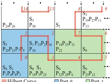
Figure 4: An example8_X8_{Hilbert Curve clustering}

The Hilbert curve-based partitioning scheme in GeoMatch acts as aglobal indexand assigns indexes to partitions such that the load is fairly distributed (i.e. query skew mitigation) and spatially close indexes are assigned to the same partition. A sample partitioning scheme is shown in Table IV.

Figure 4 depicts the clustering process and shows a partial

8_X8_{Hilbert Curve. In this example, there are}4_{streets (S}0–

S3) and 36 points (P0–P35). The figure shows the streets and points after they are partitioned. Assuming that the number of partitions is 4, then partLoad = 36

4 = 9. Indexes0 –2 are assigned topart0regardless of the fact that their count is over9. This is allowed in favor of keeping nearby objects together thus increasing accuracy. Subsequently, indexes3–7

are assigned to partition (part1), and so forth.

Querying: In order to achieve higher accuracy, the actual

distance between the two geometries must be calculated. This calculation is done locally after objects are grouped on their partitions and ultimately determines if the match is kept or discarded. The aim is to achieve results that are as close to those achieved via full map search (i.e. test each point against all streets).

VI. GEOMATCHIMPLEMENTATION

GeoMatch solves the map matching problem by matching two data sets in the form of MultiLineString (e.g. streets) and Point (e.g. GPS points). The output is a tuple consisting of a Point and a list ofk matched streets8.

GeoMatch uses a number of input configuration parame-ters like the search window (MBR) and Hilbert curve grid sizen. If the MBR is not provided, it is computed in parallel from the first input data set9. Hilbert’sn defaults to25610_.

Data Partitioning: Part of the performance gain in

Ge-oMatch comes from taking advantage of Spark’s internal PartitionerAwareUnionRDD transformation. This transfor-mation is highly efficient, migrates the smaller partition

9_{For performance gains, the smaller set should be the first input set.} 10_{The average block in NYC is}264_ft×900_{ft with an average length of}

582ft. Dividing the MBR into256yields a box size that is close to that average. The corresponding Hilbert’s curve order is 8.

Hilbert Index Count

0 88

1 41

2 29

. . . .

Table III: Index-point counts

From To Partition

1 25 0

26 30 1

31 72 2

. . . .

Table IV: Index-partition map

towards the larger one, and places the left operand data before the right one. In our experiments, this ensured that the street objects appeared before the point objects in every partition and eliminated any need for data sorting.

Hilbert Curve Indexing: The index for each object in both data sets is computed by first dividing the MBR into equal-sized n ×n boxes. Next, each Point’s single index is computed based on its coordinates. Finally, the indexes that each of street’s segments passes through are computed using a Digital Differential Analyzer (DDA) algorithm.

Load Balancing: Performance gains in GeoMatch come from distributing the load based on the data distribution such that no partition is overloaded more than others. To balance the load, first, the larger data set is read and the Hilbert index is computed for every point. Next, a list is built to show the number of points per index (e.g. Table III). Using this list, the optimal partition load is computed by dividing the sum of all points in all indexes by the total number of partitions used by the larger data set:partLoad = pointCount

partCount. The value

of partLoad indicates how many geometry points each

available partition should process. GeoMatch can exceed this limit only in favor of keeping geometries with thesame index together to increase accuracy.

Partitioning Scheme:using partLoadand the index counts list from the previous step, a partitioning scheme is built in order to spatially cluster the data sets. The scheme assigns indexes to a specific partition such that the computation load is fairly distributed acrossallpartitions while keeping spatially close indexes in the same partition (e.g. Table IV). Shuffle: Once the partitioning scheme is built, it is used to independentlypartition both RDDs. Next, the two RDDs are joined using Spark’sunion transformation which internally invokes thePartitionerAwareUnionRDDtransformation.

Querying: Map matching in GeoMatch starts after the

partitions are joined. On each partition, a local R-Tree of the streets is built in order to speed up the query process. As described earlier, our approach naturally ensures that the street objects appear before the point objects; therefore, it is easy to determine the tree’s last item. Moreover, to reduce the number of false-positive matches caused by large R-Tree MBRs, we break each street into its individual segments and insert them into the R-Tree. The segment’s MBR is expanded by a configurable value d (e.g.150ft11_{) to account for the}

Test Cores SMALL_Months

LARGE Points (Million)

SMALL Points (Million)

BUS Points (Million) 1 50 Jan–Feb 28.33 26.85 27.1 2 100 Jan–Apr 57.32 56.89 56.46 3 150 Jan–Jun 86.83 85.48 85.63 4 200 Jan–Aug 111.42 111.28 111.69 5 250 Jan–Oct 140.93 138.88 140.69

Table V: Weak Scalability experiment configurations.

inaccuracies in the initial GPS reporting.

Finally, the local R-Tree is queried and a list of candidate streets is selected for each point. Next, the distance between the point and each street is calculated; if the distance is larger than a certain limit (e.g.150ft), the match is rejected. The closestk matched streets (if any) are kept.

VII. EXPERIMENTS

We perform extensive map matching benchmarks using the data sets in Table I. The goal of each experiment is to match the points with their respective streets. Tests and anal-ysis were performed using source code obtained from the frameworks’ respective GIT repositories. To emulate real-world analyses which often operate under time and budget constraints, we consider an upper limit of 180_{minutes and}

stop any experiment if it exceeds this limit. Magellan was the only framework to consistently time out, requiring more than

180_{minutes for tasks that took}6_and9_{minutes using}

Geo-Match and GeoSpark, respectively. Additionally, the outputs of LocationSpark and GeoSpark do not include unmatched points required for error reporting and analysis. Including these points would require an additionaljoinoperation which would further increase their runtimes. GeoMatch does not suffer from this problem since it naturally passes unmatched points through its pipeline.

All experiments were conducted at the operational data facility of our research center. Our cluster consists of 20 high-end nodes each with 24TB of disk space, 256GB of RAM, and 64 AMD cores (total 1_,200+ cores) running Cloudera Data Hub 5.10 with Apache Spark 2.1.

In order to complete their tasks, LocationSpark and GeoSpark required the maximum memory allowed by our cluster –8GB for the driver and32GB for each executor. Ge-oMatch requires less memory, and we set its jobs to6_{GB for}

the driver and only8_{GB for the executor. The experiments}

measured the execution times using two different techniques. Weak Scalability – the input size and available processing power are gradually increased according to Table V and Strong Scalability – the entire data set is processed, and available processing power is gradually increased. Each test was repeated three times to accurately measure the behavior.

A. Small Taxi data set (SMALL)

In this experiment, we match points from the SMALL data set with streets from the NYC LION street data set.

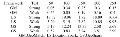
Framework Test 50 100 150 200 250 GM Strong 0.05 0.34 0.25 0.3 0.15 GM Weak 0.55 0.05 0.19 0.16 0.4

LS Strong 18.32 19.96 1.72 18.89 16.64 LS Weak 3.29 5.15 7.82 10.85 9.95 GS Strong 5.13 12.24 13.33 2.58 5.69 GS Weak 0.57 0.83 5.24 3.51 2.99

GM:GeoMatch, LS:LocationSpark, GS:GeoSpark

Table VI: Standard deviation – SMALL data set

Weak scalability:The input size and the number of

process-ing cores were gradually increased as described earlier. Fig. 5 shows the average runtimes in minutes for all experiments. GeoMatch was first to finish while producing a complete output data set. LocationSpark finished last in all cases except the one with50cores and failed all three tests using

150_{cores. Table VI shows the standard deviations.}

Strong scalability: The input size is fixed to the entire

SMALL data set (12_{months) while gradually increasing the}

processing cores from 50 _to 250 _{(in steps of} 50_{). Fig. 6}

shows the average runtimes in minutes. GeoMatch com-pleted its tasks first, followed by GeoSpark. LocationSpark was not able to process this data set with jobs either failing due to lack of memory or timing out after 180 minutes.

Table VI shows the standard deviation for all tests. It was smallest for GeoMatch, 0_.05–0_.34 minutes for strong scalability and 0.05–0.55minutes for weak scalability.

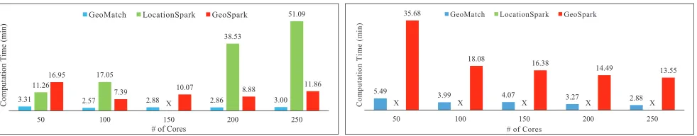
B. Large Taxi data set (LARGE)

In this experiment, we match points from the LARGE data set with streets from the NYC LION street data set. As this dataset is the largest, it requires better scalability than the other datasets. GeoMatch was able to complete all experiments within 46_{minutes, whereas none of the other}

frameworks were able to complete any experiments within

180 _{minutes. LocationSpark’s tasks either failed due to lack}

of memory or timed out. GeoSpark ran out of memory after processing20_.7_{million points (out of}3_.78_{billion) using}250

cores and maximum memory in approximately32 _minutes.

Weak scalability: Fig 7 shows the average runtimes in

minutes for all experiments. The runtimes decreased as the number of input points and processing cores increased. This indicates that GeoMatch is indeed scalable. The standard deviation of the runtimes was small (0_.15–0_.36minutes).

Strong scalability: the entire LARGE data set (3.78 Bill.

points) was used while gradually increasing the processing cores. Fig. 7 shows that the average runtimes in minutes decreased as the number of cores increased. The standard deviation of execution times was small (0.10–0.18minutes).

Output Accuracy Check: To determine the accuracy of

;

&R

P

SX

WD

WLR

Q

7L

P

H

P

LQ

RI&RUHV

*HR0DWFK /RFDWLRQ6SDUN *HR6SDUN

Figure 5: Weak Scalability Test – SMALL data set

; ; ; ; ;

&

RP

SX

WD

WLR

Q

7L

P

H

P

LQ

RI&RUHV

*HR0DWFK /RFDWLRQ6SDUN *HR6SDUN

Figure 6: Strong Scalability Test – SMALL data set

Ž

ŵ

ƉƵ

ƚĂ

ƚŝŽ

Ŷ

dŝ

ŵ

Ğ

;ŵ

ŝŶ

Ϳ

ηŽĨŽƌĞƐ

*HR0DWFK 6WURQJ6FDODELOLW\ *HR0DWFK :HDN6FDODELOLW\

Figure 7: Weak & Strong Scalability Tests – LARGE

was within150ft, the match is kept. The best10matches for each point were kept in the order of proximity. The search revealed about 10.9 million (0.30%) duplicate points and

158.9 million (4.2%) unmatched points. Full map search took 155 minutes at full processing power, 9.12 the time taken by GeoMatch (17minutes).

GeoMatch’s picks agreed with the full search97_.48% of the time, such that the three street picks were contained in the three closest matches of the full search. An additional

0.27% of results agreed with the full search starting with the 4th _{output, i.e., the three streets picked by GeoMatch}

were within the four closest matches of the full search. The full search matched an extra2.25%points over GeoMatch. We believe that this is a limitation with the DDA algorithm which approximately calculates the indexes of the streets.

C. Bus Trips data set (BUS)

In this experiment, we match points from the BUS data set with streets from the NYC LION street data set.

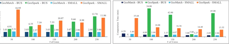
Weak scalability test: the input size and the number of

processing cores were gradually increased. Fig. 8 shows the average runtimes in minutes for the BUS and SMALL experiments for GeoMatch and GeoSpark. The runtimes for GeoMatch remained relatively stable as input size and processing power were increased. The similarities between the runtimes indicate that GeoMatch is able to efficiently handle the two types of data sets. On the other hand, GeoSpark’s runtime increased, showing worse scalability. The standard deviation of execution time was small,0_.10–

0_.31minutes and0_.09–0_.34minutes for GeoSpark.

Strong scalability test: the entire bus data set was used

while gradually increasing processing cores. Fig. 9 shows the

average runtimes in minutes for GeoMatch and GeoSpark. GeoSpark failed to complete the experiment with50 _cores,

so that result is omitted. Runtimes improved with the increase in the processing cores for GeoMatch but were erratic for GeoSpark. The standard deviation was0_.13_–0_.19

minutes for GeoMatch and0_.67–2_.62minutes for GeoSpark.

VIII. DISCUSSION

Index Accuracy:In rare cases, GeoMatch can fail to find the

optimal match if the currently matched point is located on the edge of its Hilbert cell and the optimally matching road passes through a neighboring cell. The failure rate in our experiments was rare; namely2.52%of the time. A potential way to remove these errors is to use a secondary index with coarser granularity (e.g., lower order Hilbert index) for cases where the point is close to a boundary and the shortest distance to a road is higher than the distance between the point and the boundary of the index cell.

Partitioning: Currently, GeoMatch aims to balance

parti-tions, but allows larger partitions in order to keep points of the same index together. We demonstrated that this was sufficient for data sets containing 3_.78 _{billion points, but}

when the data set size increases, further optimization may be needed. When sufficiently many computing nodes are available, we can construct a secondary nested index for partitions with a large number of points and spatial objects. Alternatively, when fewer computing nodes are available, the optimal solution is to increase the order of the Hilbert curve to achieve a better-balanced distribution of computations.

Spatial Frameworks: GeoMatch has been designed for

supporting large-scale map matching instead of being a fully-fledged spatial framework. Hence, currently, only a limited set of spatial objects, operations, and coordinate formats are supported. We plan to extend GeoMatch to support other operations and spatial data structures.

Routing: GeoMatch implements the first step in a spatial

&R

P

SX

WD

WLR

Q

7L

P

H

P

LQ

RI&RUHV

*HR0DWFK %86 *HR6SDUN %86 *HR0DWFK 60$// *HR6SDUN 60$//

Figure 8: Weak Scalability Test – BUS & SMALL

;

&

RP

SX

WD

WLR

Q

7

LP

H

P

LQ

RI&RUHV

*HR0DWFK%86 *HR6SDUN%86 *HR0DWFK60$// *HR6SDUN60$//

Figure 9: Strong Scalability Test – BUS & SMALL

should take, as well as private transport, giving drivers optimal routes to take according to the time of day and congestion conditions of the road network.

IX. SUMMARY ANDCONCLUSION

We introduced GeoMatch, a map matching method using a new spatial partitioning technique. GeoMatch is more accurate, scalable, and efficient. Compared to state of the art spatial data processing platforms for Spark, GeoMatch is1.6 –17times faster. Experimental results show that it is able to solve the map matching problem with a142GB GPS trajectory data set in about 17 minutes at full processing power while other frameworks slow considerably or fail entirely.

GeoMatch can process unstructured data, allowing pro-grams to carry meaningful non-spatial information to the map matching result without extra programming effort. It employs highly scalable indexing and load balancing tech-niques to avoid skewed data partitions, making it well suited for analysis of diverse spatial data sets that include dense city centers as well as large rural areas.

X. ACKNOWLEDGMENTS

This work was supported in part by Jorma Ollila Grant 201620040, Pitney Bowes 3100041700, and Alfred P. Sloan Foundation G-2018-11069.

REFERENCES

[1] Y. Zheng, Y. Liu, J. Yuan, and X. Xie, “Urban Computing with Taxicabs,” in Proceedings of the 13th International Conference on Ubiquitous Computing, ser. UbiComp ’11. New York, NY, USA: ACM, 2011, pp. 89–98.

[2] J. Yuan, Y. Zheng, C. Zhang, W. Xie, X. Xie, G. Sun, and Y. Huang, “T-drive: driving directions based on taxi trajec-tories,” in18th ACM SIGSPATIAL International Symposium on Advances in Geographic Information Systems, ACM-GIS 2010, November 3-5, 2010, San Jose, CA, USA, Proceedings. New York, NY, USA: ACM, 2010, pp. 99–108.

[3] B. Li, D. Zhang, L. Sun, C. Chen, S. Li, G. Qi, and Q. Yang, “Hunting or waiting? Discovering passenger-finding strategies from a large-scale real-world taxi dataset,” inIEEE PerCom 2011, 21-25 March 2011, Seattle, WA, USA, Workshop Pro-ceedings. Los Alamitos, CA, USA: IEEE, 2011, pp. 63–68. [4] Y. Huang and J. W. Powell, “Detecting regions of disequilib-rium in taxi services under uncertainty,” inSIGSPATIAL’12, Redondo Beach, CA, USA, November 7-9, 2012. New York, NY, USA: ACM, 2012, pp. 139–148.

[5] P. Shimonti, “What is Geospatial industry’s value and impact in world economy,” https://www.geospatialworld.net/blogs/ geospatial-industrys-value-world-economy/, Jan 2015. [6] J. Yu, J. Wu, and M. Sarwat, “GeoSpark: A Cluster

Com-puting Framework for Processing Large-scale Spatial Data,” in Proceedings of the 23rd SIGSPATIAL International Con-ference on Advances in Geographic Information Systems, ser. SIGSPATIAL ’15. New York, NY, USA: ACM, 2015, pp. 70:1–70:4.

[7] A. Eldawy, “Spatialhadoop: Towards flexible and scalable spatial processing using mapreduce,” in Proceedings of the 2014 SIGMOD PhD Symposium, ser. SIGMOD’14 PhD Sym-posium. New York, NY, USA: ACM, 2014, pp. 46–50. [8] “magellan,” https://github.com/harsha2010/magellan. [9] M. Tang, Y. Yu, Q. M. Malluhi, M. Ouzzani, and W. G. Aref,

“LocationSpark: A Distributed In-memory Data Management System for Big Spatial Data,” Proc. VLDB Endow., vol. 9, no. 13, pp. 1565–1568, Sep. 2016.

[10] I. Kamel and C. Faloutsos, “Hilbert tree: An improved r-tree using fractals,” inProceedings of the 20th International Conference on Very Large Data Bases, ser. VLDB ’94. San Francisco, CA, USA: Morgan Kaufmann Publishers Inc., 1994, pp. 500–509.

[11] E. S. R. Institute, “GIS Tools for Hadoop by Esri,” http://esri. github.io/gis-tools-for-hadoop/, 2018.

[12] A. Aji, F. Wang, H. Vo, R. Lee, Q. Liu, X. Zhang, and J. H. Saltz, “Hadoop-gis: A high performance spatial data warehousing system over mapreduce,”PVLDB, vol. 6, no. 11, pp. 1009–1020, 2013.

[13] H. Vo, A. Aji, and F. Wang, “SATO: A Spatial Data Partitioning Framework for Scalable Query Processing,” in Proceedings of the 22Nd ACM SIGSPATIAL International Conference on Advances in Geographic Information Systems, ser. SIGSPATIAL ’14. New York, NY, USA: ACM, 2014, pp. 545–548.

[14] S. You, J. Zhang, and L. Gruenwald, “Large-scale spatial join query processing in cloud,” in2015 31st IEEE Interna-tional Conference on Data Engineering Workshops (ICDEW). IEEE, 2015, pp. 34–41.

[15] D. Xie, F. Li, B. Yao, G. Li, L. Zhou, and M. Guo, “Simba: Efficient in-memory spatial analytics,” in Proceedings of the 2016 International Conference on Management of Data, ACM. New York, NY, USA: ACM, 2016, pp. 1071–1085. [16] S. Hagedorn, P. G¨otze, and K.-U. Sattler, “The STARK

Framework for Spatio-Temporal Data Analytics on Spark,” in Datenbanksysteme f¨ur Business, Technologie und Web (BTW 2017), 2017, pp. 123–142.