Improper Filter Reduction
Fatemeh Zahra Saberifar
∗1, A. Mohades.
†2, M. Razzazi.
‡3and J. M.
O’Kane.
§41,2Department of Mathematics and Computer Science, Amirkabir University of Technology,
Tehran, Iran.
3Department of Computer Engineering and IT, Amirkabir University of Technology, Tehran,
Iran.
4Department of Computer Science and Engineering, University of South Carolina, Columbia,
South Carolina, USA.
ABSTRACT ARTICLE INFO
Combinatorial filters, which are discrete representations of estimation processes, have been the subject of increas-ing interest from the robotics community in recent years. This paper considers automatic reduction of combinato-rial filters to a given size, even if that reduction necessi-tates changes to the filter’s behavior. We introduce an algorithmic problem called improper filter reduction, in which the input is a combinatorial filter F along with an integer k representing the target size. The output is another combinatorial filter F0 with at most k states, such that the difference in behavior between F and F0
is minimal. We present two methods for measuring the distance between pairs of filters, describe dynamic
Article history:
Received 08, February 2018 Received in revised form 05, May 2018
Accepted 27 May 2018
Available online 01, June 2018
Keyword: combinatorial filters; estimation; automata
AMS subject Classification: 05C78.
†Corresponding author: A. Mohades. Email: [email protected] ‡[email protected]
1
Abstract continued
programming algorithms for computing these distances, and show that improper filter reduction is NP-hard under these methods. We then describe two heuristic algorithms for improper filter reduction, one greedy sequential approach, and one randomized global approach based on prior work on weighted improper graph coloring. We have implemented these algorithms and analyze the results of three sets of experiments.
2
Introduction
This paper builds upon the ongoing line of research on combinatorial filtering for robot tasks [19,31,37]. The intuition of that work is to carefully design filters that robots or other autonomous agents can use to retain only the information that is strictly necessary for completing an assigned task. This class of filters is applicable for any task that can be characterized by discrete transitions triggered by finite sets of observations.
Recent research has considered the problem of automatic reduction of combinatorial fil-ters: Given a combinatorial filter that correctly solves a problem of interest, can we algorithmically find the smallest equivalent filter? Prior work showed that this problem is NP-hard and described an efficient heuristic algorithm for finding small—but not nec-essarily the smallest—equivalent filters [21]. However, that prior work left a number of important questions unanswered, including these:
Is there a useful notion of the behavior of a reduced filter being “close enough” to the original filter? If so, then given an input filter, can we find the most similar filter of a given fixed size?
We refer to this problem as the improper filter reduction problem.1 This paper addresses
that problem, making several new contributions.
1. We introduce a family of distance functions for measuring the difference between filters and describe dynamic programming algorithms for computing these distances.
2. We argue that, for any distance function, the improper filter reduction problem is NP-hard.
3. We present two algorithms for improper filter reduction. These are heuristic algo-rithms, in the sense that there is no guarantee that their output will fully minimize the distance from the original filter.
4. We present implementations of these algorithms, along with a series of experiments evaluating their performance.
1
n n−1
2
. . .
. . .
{1}
{2,3}
...
{n−1, n} {2}
...
{n}
{1, n}
{1,2} {1, . . . , n}
1, n
1, n
2, . . . , n−1
1, n−1
n
2, n
1 2, . . . , n−1
n
1
{1, . . . , n} {1, n−1} {1,2}
{2,3}
...
{n−1, n} {2}
...
{n} {1}
1, n 2, . . . , n−1
2, . . . , n−1
1, n
2, . . . , n−1 1, n
Figure 1: [top left] An agent moves through an annulus divided into n regions by n
beam sensors. [top right] The smallest filter, found by a prior algorithm [21], that can accurately track whether the agent is provably within region 1 or not. [bottom] A smaller filter produced, for any specific value of n, by the algorithm introduced in this paper. This reduced filter eliminates the extra states for region sets {1, n} and {1,2}, which are used only at the start.
These answers are relevant not only because they can help to reduce the memory needed to execute a combinatorial filter, but also because they may provide some insight into one of the fundamental tasks in robot design, namely understanding how a robot should process and retain information collected from its sensors.
Figure 1 shows a simple example, in which an agent moves through a ring-shaped en-vironment along a continuous but unpredictable path. A collection of n beam sensors, numbered 1, . . . , nis spread through the environment. These sensors can detect the agent passing by, but cannot determine whether that crossing was in the clockwise or counter-clockwise direction. One pair of beams delimits a special “goal” region, called region 1 and delimited by beams 1 and n. A natural question for this system is to ask what kinds of filters can determine when the agent is within region 1. That is, we are interested in designing filters —expressed as transition graphs, with edges labelled by beam crossings and states labelled by outputs— whose outputs indicate whether the agent is known to be in region 1 or not.
In fact, it is possible to form a many different of filters. Some examples:
2n−1 nodes, each representing a nonempty set of “possible states,” with directed
edges indicating how the possible states change with each beam crossing. In that filter, we would choose the state corresponding to {1, . . . , n} as the initial state. The filter’s output would be defined as “yes” for the state corresponding to the set {1}—indicating that only state 1 is consistent with the history of observations—and “no” for each other state.
• That na¨ıve filter can be made more compact by noticing that, ifn >3, only 2n+ 1 of those nodes can ever be reached: One initial state in which all regions are possible states; one state for each beam, in which only the two regions on opposite sides of that beam are possible states; and one state for each region, in which the agent is known to be in that region. The remaining 2n−2n −2 nodes can be discarded
without changing the filter’s outputs, because no observation sequence can reach them.
• That filter can be reduced even further, again without changing its outputs, by a sequence of vertex contractions. Prior work shows that selecting those vertex contractions optimally is, in general, NP-hard [21], but also presents an efficient algorithm that performs this reduction well in practice. The resulting filter, which has 5 states regardless of the number of beams, is shown in the top portion of Figure 1.
• This paper is concerned with additional reductions beyond this smallest equivalent filter, which requires us to tolerate some “mistakes” in which the filter produces in-correct outputs for some observation sequences. Thus, the reduction is “improper.” The bottom portion of Figure 1 shows how the algorithm introduced in this paper can reduce the filter to three states, corresponding to “in region 1”(shown on the right), “not in region 1” (middle), and “maybe” (left). The filter may produce in-correct outputs for some observation sequences—One such observation sequence is 1, n, n,1,1, n, n, . . .— but behaves the same as the original after the first beam not adjacent to region 1 is crossed.
This paper examines the algorithmic problems latent in the final step of this series of reductions. The objective is to understand the tradeoffs between a filter’s size and its ability to produce correct outputs.
3
Related Work
3.1
Combinatorial filters
Combinatorial filters are a discrete formalization of processes that aggregate, fuse, and process data collected by sensors. As a general class, they build upon the information space formalism popularized by LaValle [18,19]. The central idea is to perform filtering tasks in very small derived information spaces, thereby minimizing the computational bur-den of executing the filter, and illuminating the structure underlying the problem itself. Recent work describes combinatorial filters for navigation [20,31], target tracking [37], validation [35,36], and localization [1] problems. Tovar, Cohen, Bobadilla, Czarnowski, and LaValle [32,33] introduced optimal combinatorial filters for solving some inference tasks in polygonal environments with beam sensors and obstacles. Kristek and Shell [17] showed how to extend existing methods for sensorless manipulation [10,12] to deformable objects. Song and O’Kane [29] investigated extensions to limited classes of infinite in-formation spaces. The deterministic filters we define in this paper are an special case of nondeterministic graphs explored using topological methods by Erdmann [8,9], in the context of planning under uncertainty.
3.2
Filter reduction
The common thread through all of the prior work mentioned so far is to rely on hu-man analysis generate efficient filters for specific problems. The first results on finding optimal filters automatically were presented by O’Kane and Shell [21,22]. They proved that the filter minimization problem is NP-hard and presented a heuristic algorithm to solve it. The same authors also used similar techniques to solve concise planning [21,23] and discreet communication [24] problems. The present authors extended those results by considering fixed-parameter tractability, hardness of approximation, and a number of special cases [27]. This paper continues that work by addressing the case in which the reduced filter need not be strictly equivalent to the original.
Our problem also has some similarity to the problem of measuring the similarity of two deterministic finite automata, as considered by Schwefel, Wegener, and Weinert [28], who solved it using evolutionary algorithms. Chen and Chow also used a scheme for comparing automata, specifically in the context of web services [6]. Our work is differs because of the unique challenges inherent in the differences between filters and automata—because the behavior of a filter may be undefined for certain state-action pairs, the problem of measuring similarities between filters is more challenging.
3.3
Probabilistic methods
system, in which the state of the system corresponds to the robot’s “belief” about the cur-rent state of the world, and transitions between such states are triggered by observations. The primary difference is that for combinatorial filters, we generally assume that both the state space and the observation space are finite, which enables a number of interesting algorithmic questions—including, for example, the filter reduction problem addressed in this paper—to be reasonably posed.
There exists some research in automatic probabilistic motion planning using partially-observable Markov decision process (POMDP) models. Roy, Gordon, and Thrun applied dimensionality-reduction techniques to reduce the computation needed for effective plan-ning under such models [25]. Ballesteros, Wegener, and Weinert [4] improved the efficiency of online POMDPs in planning task by reduction of similar belief points. Crooket al. [7] also presented an automatic POMDP-based approach for belief space compression.
4
Definitions and Formulation
This section provides basic definitions for combinatorial filters and the improper filter reduction problem.
4.1
Filters and their languages
A robot receives a discrete sequence of observations, drawn from a finite observation space. Each observation represents a single sensor reading or a passively-observed action taken by the robot. In response to each of these observations, the robot produces an output, in-formally called a color. We model this type of system as a transition graph. Each vertex of the transition graph represents the knowledge, called an information state, retained by the robot at some particular time. Each directed edge is labeled with an observa-tion, showing how the information state changes in response to incoming observations. Definition 4.1 formalizes this idea.
Definition 4.1. A filter F = (V, E, l, Y , c, Cout, q0) is 7-tuple, representing a directed
graph with labels on both its vertices and edges, in which
• the set V is a finite set of vertices calledinformation states or simply states,
• the multiset E is a finite collection of ordered pairs of states, called transitions, in which every state has at least one out-edge,
• the function l : E → Y assigns a label l(e) to each edge e ∈ E, such that no two edges share both a source vertex and a label,
• the function c : V → Cout assigns value c(q) drawn from a finite color space Cout,
informally called thecolor of q, to each state q ∈V, representing the output of the filter at that state, and
• the vertexq0 ∈V is called the initial state.
Definition 4.1 makes two important assumptions about the edges in a filter. First, it requires that no two edges originating from the same vertex can share the same label. Thus, given a “current” state and a new observation, there is at most one resulting state reached by following the edge labeled with that observation.2 Second, the definition does
not require that there must be an outgoing edge for each observation from each vertex. This corresponds to situations in which, based on the underlying structure of the problem, the robot is certain that a given observation cannot occur from a given state.
During its execution, the filter starts at the initial state q0 and immediately outputs
c(q0). After each observation y, the filter transitions from its current state q to a new
state q0, following the edge q −→y q0, if that edge exists. The filter then generates a new
output, namely c(q0), and awaits the next observation. For a given observation string
s=y1y2· · ·ym, there are two cases:
1. If all of the corresponding edges exist, then filter’s output is a sequence of m+ 1 colors. We write, in a slight abuse of notation, F(s, q) denote the output sequence generated when the filter F processes s starting from state q. We also use the shorthand F(s) to denote F(s, q0).
2. If the filter ever reaches a current state for which no out-edge is labeled with the next observation, we say that the filter has failed for this input, and the filter output is undefined.
The goal of this paper is to understand, given a filter that acts as a “specification” of the desired output, how to find small filters that produce the substantially similar outputs. However, this comparison only makes sense for observation sequences for which the output of the original filter is well-defined. The next definition formalizes this idea.
Definition 4.2. The language L(F) of a filterF is the set of all observation sequences s
for which F(s) is well-defined.
4.2
Defining distance between filters
Given two filters F1 and F2 with the same observation space Y, we define the distance
between F1 and F2 by considering their operation on identical observation strings, and
quantifying the difference between the corresponding output strings. Specifically, we choose a function m : S
i∈N(Couti ×Couti) → R+, representing a metric
that measures the distance between two equal-length output strings. We consider, both
in the algorithms of Section 5 and the experiments in Section 8, two specific options for
m:
1. Hamming distance [14], denoted h, which counts the number of positions at which the two strings differ.
2. Edit distance [34], denoted e, which is the smallest number of single-character insert, delete, and substitute operations, weighted by given operation costs cins, cdel, and
csub respectively, needed to transform one string into another.
Then, given two filtersF1 and F2, for which L(F1)⊆L(F2), we use this distance function
over observation strings —either m = h or m = e— to define the distance Dm(F1, F2)
between F1 and F2:
Dm(F1, F2) = sup
s∈L(F1)∩L(F2)
m(F1(s), F2(s))
length(s) + 1
. (1)
The intuition is to consider the worst case distance between output strings, over all observation strings in L(F1)∩ L(F2)—that is, over all observation strings that can be
processed by both filters—normalized by the length of the output strings. The use of worst-case reasoning allows us to compare filters without the modelling burden of assigning probabilities to observation sequences. Normalization is necessary to ensure that the distance between filters is finite. Because the denominator represents the length of both
F1(s) andF2(s)—that is, one more output than there are observations—this can be viewed
as an “average cost-per-stage” model as described by LaValle [18].
4.3
Improper filter reduction
We can now state the central algorithmic problem addressed in this paper.
Problem: Improper-FM
Input: A filter F and an integerk.
Output: A filterF0with at mostkstates, such thatL(F)⊆L(F0) andD
m(F, F0)
is minimal.
Note, however, that this problem is NP-hard, regardless of the choice ofm. The proof is straightforward.
Theorem 4.3. Improper-FM is NP-hard.
Proof. Reduction from the basic (error-free) filter minimization problem,FM[21]. Given
an instanceF ofFM, one can use binary search on the range{0, . . . , n}to find the smallest
value of k for which there exists an F0 with L(F) ⊆L(F0) and Dm(F, F0) = 0. This F0
is, by definition, the correct output for FM. Therefore, a polynomial time algorithm for Improper-FMwould imply a polynomial time algorithm forFM. SinceFMis NP-hard,
and we have a polynomial-time reduction from FM to Improper-FM, conclude that
Consequently, we restrict our attention in this paper to heuristic algorithms that attempt, but cannot guarantee, to minimize the distance between the reduced filter and the original.
5
Computing distance between filters
Before turning our attention to Improper-FM, we first consider the related problem of
computing the distance Dm(F1, F2) between a given pair of filtersF1 and F2. Attempting
to evaluate Equation 1 directly would be futile, because it includes a supremum over
L(F1)∩L(F2), which in general may be an infinite set. Instead, we introduce a dynamic
programming [5] algorithm whose outputs converge to Dm(F1, F2). The details of the
algorithm for computing Dm(F1, F2) differ depending on whether the underlying string
distance function m is Hamming distance function h (addressed in Section 5.1) or edit distance function e (addressed in Section 5.2).
5.1
Hamming distance based method
Our algorithm for computingDh(F1, F2) is based on computing successive values of a
sim-pler functiondh, which only considers observation strings up to a certain given length. Our
algorithm considers longer observation strings at each iteration. To facilitate a dynamic programming solution, we also must consider different starting states for each filter.
Definition 5.1. Let dh(q1, q2, k) denote the maximum, over all strings s of length k in
L(F1)∩L(F2), of h(F1(s, q1), F2(s, q2)), or 0 if there are no such strings.
The functiondh is useful because values forDh can be derived from values ofdh, as shown
in the next lemma.
Lemma 5.2. For any two filters F1 and F2, with initial states q01 and q02 respectively,
and with L(F1)⊆L(F2), we have
Dh(F1, F2) = lim
k→∞
max
i∈1,...,k
dh(q01, q02, i)
i+ 1
.
Proof. For any >0, we must show that, for sufficiently large k, we have
Dh(F1, F2)− max
i∈1,...,k
dh(q01, q02, i)
i+ 1
< .
First, we note that, for anyk, we have
Dh(F1, F2) ≥ max
i∈1,...,k
dh(q01, q02, i)
i+ 1 ,
For the other direction, we let s denote an observation string for which
Dh(F1, F2)−
h(F1(s), F2(s))
length(s) + 1 ≤. (2)
Such a string must exist by the definition of supremum. Then, choosing k = length(s), we have
max
i∈1,...,k
dh(q01, q02, i)
i+ 1 ≥
h(F1(s), F2(s))
k+ 1 ≥Dh(F1, F2)−. (3) In Equation 3, the first step holds because the specific string s is among the strings considered in the maximum over all strings of length at most k, and the second steps proceeds directly from Equation 2. Therefore, the difference between Dh(F1, F2) and
maxi∈1,...,kdh(q01, q02, i)/(i+ 1) is at most , completing the proof.
When k = 0, the filter receives no observations and produces a single output, so dh is
trivial to compute in this case, depending only on whether the single outputs produced by each filter match each other:
dh(q1, q2,0) =
(
0 ifc1(q1) =c2(q2)
1 otherwise . (4)
Next we address the general case in which k > 0. From any state pair (q1, q2), we must
consider the set of observations for which both q1 and q2 have outgoing edges, denoted
Y(q1, q2). Thus, for any observation in Y(q1, q2), we know that there exists an edge
q1
y −→q0
1 in F1 and an edge q2
y −→q0
2 in F2, labeled with the same observation y. Then
we can expressdh(q1, q2, k) recursively in terms ofdhvalues with shorter observation string
lengths:
dh(q1, q2, k) = max
y∈Y(q1,q2)
(dh(q1, q2,0) +dh(q01, q20, k−1)), (5)
in whichq0
1 denotes the state inF1 reached when observation y occurs from state q1, and
likewiseq0
2 denotes the state inF2 reached when observationyoccurs from stateq2. When
Y(q1, q2) is empty, we usedh(q1, q2, k) = 0. (The intuition of this special case is that, in
this case, q1 and q2 are a good choice to merge, because when forming a reduced filter in
which q1 is merged withq2, there will be no ambiguity in selecting the correct destination
for any transition from the combined state.)
Algorithm 1 shows the dynamic programming algorithm that uses this recurrence to compute Dh(F1, F2). The intuition is to computedh for increasing values of k, until those
dh values converge, and then to find the appropriate normalized maximum.
5.2
Edit distance based distance
We now turn to algorithms that, given two filters F1 and F2, compute De(F1, F2). The
approach is similar to the approach for Dh in Section 5.1. However, the algorithm for De
is more complex because it must account for the different-length strings that can arise from insert and delete operations on the output sequences.
Algorithm 1: Dynamic programming to compute Dh(F1, F2).
k ←0
repeat
done←True
for (q1, q2)∈V1×V2 do
Compute dh(q1, q2, k) using Eq. 4 or 5.
if
dh(q1,q2,k)
k+1 −
dh(q1,q2,k−1)
k
> then done←False
end end
k ←k+ 1
until done
return max
i=0,...,k−1
dh(q01, q02, i)
i+ 1
Definition 5.3. Let de(q1, k1, q2, k2) denote the largest edit distance between F1(s1, q1)
and F2(s2, q2), over all strings s1 of length k1 and all strings s2 of length k2, for which
s1, s2 ∈ L(F1)∩L(F2), and s1 and s2 are identical to each other for the first min(k1, k2)
observations.
We can show that de is useful for computingDe with a lemma analogous to Lemma 5.2.
Lemma 5.4. For any two filters F1 and F2, with initial states q01 and q02 respectively,
and with L(F1)⊆L(F2), we have
De(F1, F2) = lim
k→∞
max
i∈1,...,k
de(q01, i, q02, i)
i+ 1
.
Proof. For any >0, we must show that, for sufficiently large k, we have
De(F1, F2)− max
i∈1,...,k
de(q01, i, q02, i)
i+ 1
< .
In other words, we need to proof that
− < De(F1, F2)− max
i∈1,...,k
de(q01, i, q02, i)
i+ 1 < . (6)
As an observation, note that for any k, the following inequality is true,
De(F1, F2) ≥ max
i∈1,...,k
de(q01, i, q02, i)
i+ 1 ,
to L(F1)∩L(F2) and the right side is defined over all observation strings belonging to
L(F1)∩L(F2) with length of at most k.
Thus, we just need to show the right side of Equation 6. For this purpose, let there be an observation strings for which
De(F1, F2)−
e(F1(s), F2(s))
length(s) + 1 ≤. (7)
Such a string must be exist by one of the main properties of supremum definition. Then, letk = length(s), we have
e(F1(s), F2(s))
k+ 1 ≤i∈max1,...,k
de(q01, i, q02, i)
i+ 1 , (8)
because the string s is one of the all strings with length of at most k. Now, from Equation 7 and 8, we have
De(F1, F2)−≤
e(F1(s), F2(s))
k+ 1 ≤i∈max1,...,k
de(q01, i, q02, i)
i+ 1 . (9)
Therefore, from Equation 9, we conclude the right side of Equation 6.
The fact thatde considers observation sequences of different lengths is irrelevant, because
the limit in Equation 5.4 uses the same value, namely k1 = k2 = i, for the two string
lengths and we know that, based on the relation between the Hamming distance and the edit distance, when k1 =k2 =i, we have de(q01, i, q02, i)≤dh(q01, q02, i).
We can now construct a recurrence forde. There are three base cases.
1. When k1 = 0 and k2 = 0, both filters produce a single output. Editing one such
string into the other can be one either by a substitution, or by one deletion and one insertion:
de(q1,0, q2,0) =
(
0 if c1(q1) =c2(q2)
min(csub, cdel+cins) otherwise
. (10)
2. When k1 = 0 and k2 > 0, we have a single character c(q1) of output from F1 and
a longer output string F2(s2, q2), with length k2 + 1, from F2. The edit distance
between these strings depends on whether c(q1) appears in F(s2, q2). If c(q1) does
not appear in F(s2, q2), then we need either (a) 1 deletion and k2 + 1 insertions or
(b) 1 substitution andk2 insertions, whichever has smaller total cost. Ifc(q1) does
appear in F(s2, q2), then c(q1) can be ‘reused’ in F(s2, q2), reducing the edits to
simply k2 insertions.
Because Definition 5.3 calls for the largest edit distance, the relevant question is whether there exists any sequence of observations which, when given as input to
L(q2, c(q1)) denote the length of the longest path in F2 starting from q2 that does
not visit any states of color c(q1).3 We can expressde for this case as:
de(q1,0, q2, k2) =k2cins+
(
min(cdel+cins, csub) ifL(q2, c(q1))> k2
0 otherwise (11)
3. When k1 > 0 and k2 = 0, the situation is analogous, but with the roles of F1 and
F2 swapped:
de(q1, k1, q2,0) =k1cdel+
(
min(cins+cdel, csub) if L(q1, c(q2))> k1
0 otherwise (12)
In the general case, we can express values fordeusing a recurrence similar to the standard
recurrence for edit distance [34], but accounting for the changes in state that accompany each observation. For given values of q1, k1, q2, and k2, we must consider the worst case
over all observations for which both q1 and q2 have outgoing edges. As in Section 5.1,
we write Y(q1, q2) to denote this set of observations, and for each y ∈ Y(q1, q2) we write
q1
y −→q0
1 and q2
y −→q0
2 for the two corresponding edges. To compute de(q1, k1, q2, k2), we
consider the worst case over all observations y ∈Y(q1, q2):
de(q1, k1, q2, k2) = max
y∈Y(q1,q2)
d(y)
e (q1, k1, q2, k2), (13)
in which we have introduced a shorthand notation d(ey) for the value of de predicated
receiving a specific observation y next. There are two cases ford(ey).
1. If c1(q1) =c2(q2), no edits are needed, so we have
de(y)(q1, k1, q2, k2) = de(y)(q01, k1−1, q20, k2 −1).
2. If c1(q1)6=c2(q2), we use the smallest cost from among insert, delete, and substitute
operations:
d(ey)(q1, k1, q2, k2) = min
de(q1, k1, q02, k2−1) +cins,
de(q10, k1−1, q2, k2) +cdel,
de(q10, k1−1, q02, k2−1) +csub
.
The intuition is that, in the case of a delete, F1 will process one observation,
tran-sitioning from q1 toq10 and reducing the length of the remaining observation string
by 1, whereas F2 does not process any observations, remaining in state q2, with
the same number of observations remaining. For an insert, F2 will process one
Algorithm 2: Dynamic programming to compute De(F1, F2).
i←0
repeat
done←True
for j ←0, . . . , i do
for (q1, q2)∈V1×V2 do
Compute de(q1, i, q2, j) using Eq. 10, 11, 12, or 13.
Compute de(q1, j, q2, i) using Eq. 10, 11, 12, or 13.
end end
for (q1, q2)∈V1×V2 do
if
de(q1,i,q2,i)
i+1 −
de(q1,i−1,q2,i−1)
i
> then done←False
end end
k ←k+ 1
until done
return max
i=0,...,k−1
de(q01, i, q02, i)
i+ 1
observation, transitioning from q2 to q20 and reducing the length of the remaining
observation string by 1, whereas F1 does not process any observations, remaining
in state q1, with the same number of observations remaining. For a substitution,
both F1 and F2 transition to new states, and both k1 and k2 are decreased. This
corresponds to the usual recurrence for edit distance.
This recurrence leads directly to an algorithm for computing De(F1, F2). Pseudocode
appears as Algorithm 2. The algorithm applies the recurrence, starting from k1 =k2 =
0, and increasing those indices until the average error per observation converges, as in Lemma 5.4. The most important subtlety is in the ordering: Before computingde values
with input string lengths (k1, k2), we must ensure that the corresponding computations
have been completed for (k1−1, k2), (k1, k2−1), and (k1−1, k2−1).
Note that Algorithm 2 is significantly slower than Algorithm 1 because of the need for an additional nested loop to accommodate the differing string lengths between F1 and F2.
This difference, which we also observe in the experiments described in Section 8, confirms the basic intuition that Hamming distance is a computationally simpler string distance than edit distance. Note, however, that edit distance is a more ‘forgiving’ distance, in the sense that if cins = cdel = csub = 1, then De(F1, F2) ≤ Dh(F1, F2) for any two filters F1
6
Local greedy sequential reduction
In this section, we present a heuristic algorithm for improper filter reduction that effi-ciently reduces the input filter to the required size, while attempting to minimize the error. The algorithm performs a series of greedy “merge” operations, each of which reduces the filter size by one. We first describe the details of this merge operation (Section 6.1), and then propose an approach for selecting pairs of states to merge (Section 6.2).
6.1
Merging states
Suppose we have a filter F withn states, and we want form a new, nearly identical, filter
F0 with n−1 states. One way to accomplish this is to select two states q
1 and q2 from
F—deferring to Section 6.2 the question of how to select q1 and q2—and merge them, in
the following way.
• Replace q1 and q2 with a combined state, denoted q1,2. If either of q1 or q2 is the
filter’s initial state, then q1,2 becomes the new initial state. We assign the color of
q1 to the combined state q1,2.
• Replace each in-edge qi y
−→ q1 of q1, with a new edge qi y
−→ q1,2 to the combined
state. Repeat for q2, replacing each qi y
−→q2 with qi y −→q1,2.
• Replace each out-edge q1
y
−→qj of q1 with a new edge q1,2
y −→qj.
• For each out-edge q2
y
−→ qj, determine whether q1 has an out-edge with the same
label y. If so, then discard the edge q2
y
−→qj. If not, then replace that edge with
q1,2
y −→qj.
The intuition is to replace the two states q1 and q2 with just one state, with as little
disruption to the filter as possible. The only complication—and the reason that this merge operation must be more complex than a standard vertex contraction—is that the combined node can have at most one out-edge for each observation label. When q1 and
q2 both have out-edges with the same label, we arbitrarily resolve that conflict by giving
priority to q1 overq2.
In the context of the Improper-FM problem, we also must ensure that the filter F0
resulting from a merge in F has L(F) ⊆ L(F0). This may not be immediately true, as
illustrated in Figure 6.1. To resolve this problem, we perform a forward search over state pairs (qa, qb), in which qa is from the original filter F and qb is from the merged filterF0,
starting from (q2, q1,2) when we suppose that q2 is merged into the q1 to createq1,2. Each
time this search finds a reachable state pair (qa, qb) and an observationy, for whichF has
an edge qa y −→ q0
a but F0 has no edge from qb labeled y, we insert an edge qb y −→q0
a into
F0. This ensures that any observation sequence that can be processed by F can also be processed by F0. The runtime of this post-processing step is quadratic in the number of
q1 q2
y2 y2
y0 y1
y3 y4
q1,2
y2
y0, y1
y3 y4
q1,2
y2
y0, y1
y3, y4 y4
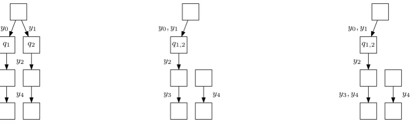
Figure 2: An illustration of the need for post-processing after merging two states q1 and
q2, to ensure that L(F) ⊆L(F0). [left] A filter F, before q1 and q2 are merged. [center]
Another filter F0, formed by combining q
1 with q2, but without post-processing. In this
example, F can process the observation string y1y2y4, but F0 fails on that input. [right]
The post-processing step adds an edge to resolve the problem.
We write merge(F, q1, q2) to denote the filter resulting from applying this complete merge
operation to q1 and q2 inF.
6.2
Selecting pairs of states to merge
We can use this merge operation to form a heuristic algorithm for improper filter reduction in a local greedy way. The basic idea is to consider all ordered pairs of distinct states in the current filter as candidates to merge, and to compare the filter resulting from each such merge to the original input filter. The merge that results in the smallest distance from the original filter is kept, and the algorithm repeats this process until filter is reduced to the desired size. If there are multiple candidates with same distances to the original filter, we choose one of them arbitrarily.
Beyond this basic idea, we add two additional constraints to improve the quality of the final solution. First, we reject any merge operation that leaves some states unreachable, unless all available merges leave at least one unreachable state. Second, we also reject any merge operation that eliminates at least one output color from the resulting filter, unless all available merges eliminate a color. Algorithm 3 shows the complete approach. See Section 8 for an evaluation of this algorithm’s effectiveness.
7
Randomized global reduction
Algorithm 3: A greedy sequential method to reduce F tok states.
f ←False
Forig ←F
while |V(F)|> k do
D? ← ∞
for (q1, q2)∈V(F)×V(F) do
if q1 =q2 then
continue end
F0 ←merge(F, q1, q2)
if f =False then
if F0 has unreachable states then continue
end
if F0 has unreachable colors then continue
end end
D←Dm(Forig, F0) // Use Alg. 1 or Alg. 2.
if D < D? then
D? ←D
F? ←F0 end
end
if D? =∞then
f ←True
end else
f ←False
F ←F?
existing algorithm (Section 7.1). We then apply a randomized ‘voting’ process to construct the reduced filter from the colored graph (Section 7.2).
Algorithm 4: A randomized global method to reduce F to k states using r itera-tions.
C ←C(F)
c← improper coloring of C with k colors[2].
D? ← ∞
for R←0, . . . , r do
F0 ← empty filter
for each color i in c do
q ←state in F randomly selected from those coloredi in C(G) Create a state qi in F0 with same output color as q.
end
for each color i in c do
for each observation y ∈Y in F do
q ←state in F randomly selected from those both colored i inC(G) and with an edge q−→y w inF.
Create an edge in F0 from qi toqc(w) labeled y.
end end
D←Dm(F, F0) // Use Alg. 1 or Alg. 2.
if D < D? then
D? ←D
F? ←F0 end
end return F?
7.1
Selecting merges via improper graph coloring
We can view the problem of reducing a given filter F down to k states as a question of partitioning the states of F into k groups. Our algorithm accomplishes this by solving a coloring problem on a complete undirected graph C(F), defined as follows:
1. For each state q in F, we create one vertex v(q) in C(F).
2. For each pair of distinct vertices v(q1), v(q2) in C(F), we create a weighted edge.
The intuition is that the weights should be estimates of how different the two cor-responding states are. If the behavior of F is very similar when started from q1 as
when started from q2, then we should assign a relatively small weight to the edge
A B C E D a
b,c,d
e
a
b,e
b,c,d
a,e a,e
a,d
e A B C D E
0.66
0.66
0.5 0.33
0.66 0.5 0.5
0.5
0.5
0.5
Figure 3: [left] An example five-state filter. (This filter was originally generated by the algorithm of O’Kane and Shell [21]. [right] The corresponding complete graph, along with an improper coloring of that graph with two colors.
started from q1 compared to starting from q2, then we should assign a relatively
large weight to that edge.
We can capture these kinds of differences by computing the distance of F with itself—That is, by computing either Dh(F, F) orDe(F, F)—and examining the
in-termediate values—either dh(q1, q2, k) orde(q1, k, q2, k), in whichk is the number of
iterations of the outermost loops in Algorithm 1 or Algorithm 2—computed along the way. Specifically, we assign w(q1, q2) as
w(q1, q2) = lim
k→∞
max
i∈1,...,k
dh(q1, q2, i)
i+ 1
for Hamming distance, and
w(q1, q2) = lim
k→∞
max
i∈1,...,k
de(q1, i, q2, i)
i+ 1
for edit distance.
Figure 3 shows an example of this construction.
The idea is then to assign a color c(v) to each vertex v of C(F), using at most k colors, while minimizing the worst case over all vertices, of the total weight of edges to same-colored neighbors. That is, we want assign k colors to the vertices of C(F) in a way that minimizes this objective function:
O(F, c) = max
v∈V(C(F))
X
{u∈V(C(F))−{v} |c(v)=c(u)}
w(u, v), (14)
Bermond, Giroire, Havet, Mazauric and Modrzejewski [2]. Though the problem is NP-hard even to approximate—Note that an efficient algorithm for this problem could be used to build an efficient algorithm for the standard proper graph coloring problem—that prior research presents a randomized heuristic algorithm that performs well in most cases. We use that algorithm to color C(F).
7.2
Randomized voting for improper filter reduction
Next, we form the reduced filter F0 by ‘merging’ the states in F corresponding to each
group of same-colored nodes in C(F) into a single state in F0. The process is somewhat analogous to pairwise merging process described in Section 6.1, but must account for some important differences. Most importantly, because we want to merge the states within each of the k color groups simultaneously, when selecting the edges in the reduced filter F0, it only needs to consider which state in F0—that is, which color group—should be the
target of that edge, rather than making a finer-grained selections of some state in some partially-reduced version of F.
Note, however, that the states in each color group may not agree on whichF0 state should
be reached under each observation. When, for a given observation y, such disagreements occur, we resolve them in a randomized way. The algorithm selects, using a uniform random distribution, one of the F states in this color group that has an edge labeled with y, and adds a transition in F0 the state corresponding to the color group reached
by that state. This forms a kind of ‘weighted voting,’ in which it is more likely to select transitions that correspond to larger number of states in the group.
Similarly, we select the output color of each state in F0 by randomly selecting one of its
constituent states and using its color as the output for the combined state. Continuing the example from Figure 3, observe that to create reduced filter with two states, one of those states will correspond to the original filter’s A, B, and C states, and other one will consist of D and E. Since D and E have different colors in the original filter, the algorithm assigns the new DE state to each of the two possible output colors with equal probability. Because the final filters produced by this process are not deterministic, we repeat the reduction several times and return the best filter resulting from those iterations.
8
Implementation and Experimental Results
We have implemented Algorithms 1–4 in Python. The experiments described below were
executed on a GNU/Linux computer with a 3GHz processor. Throughout, we used =
0.035 in Algorithms 1 and 2, cins = cdel = csub = 1 in Algorithm 2, and r = 400 in
Algorithm 4.
8.1
Distance and run time for varying filters
annulus-shaped environment, occasionally crossing a beam sensor that detects a crossing of that beam has occurred, but cannot detect which robot has crossed, nor the direction of that crossing. The filter should process these observations and output 0 if the robots are together, or 1 if the robots are separated by at least one beam. (This is a different and more challenging problem than the single-robot variant described in Section ??.)
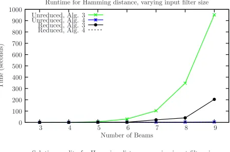
We varied the number of beam sensors from 3 to 9, and tested two equivalent filters for each number of beams: one ‘unreduced’ na¨ıve filter, formed by directly computing the sets of possible states after each observation, and a smaller ‘reduced’ filter produced by applying the algorithm of O’Kane and Shell [21] to the unreduced versions. These reduced filters have the same behavior as their unreduced counterparts, but are the smallest filters for which that equivalence holds.
For each of these 7·2 = 14 filters, we executed both Algorithm 3 and Algorithm 4, using bothDh and De as the underlying distance for each algorithm. The target filter size was
set to k = 2, the maximal meaningful reduction, for each of these trials. The results appear in Figure 4 for Hamming distance and in Figure 5 for edit distance.
These results show that the final solution quality is somewhat better for Algorithm 4 in many cases. The global approach of Algorithm 4 is also faster than the greedy sequential reduction of Algorithm 3. The difference, which is especially pronounced as the filter size grows large, is explained by the fact that Algorithm 4 uses its subroutine for distance between filters—that is, Algorithm 1 or 2—only once, rather than many times for each reduction.
Unreduced, Alg. 3
Unreduced, Alg. 4
Reduced, Alg. 3
Reduced, Alg. 4
0
100
200
300
400
500
600
700
800
900
1000
3
4
5
6
7
8
9
T
im
e
(s
ec
on
d
s)
Number of Beams
Runtime for Hamming distance, varying input filter size
Unreduced, Alg. 3
Unreduced, Alg. 4
Reduced, Alg. 3
Reduced, Alg. 4
0.0
0.1
0.2
0.3
0.4
0.5
0.6
0.7
0.8
0.9
1.0
3
4
5
6
7
8
9
D
h(
F
,F
′
)
Number of Beams
Solution quality for Hamming distance, varying input filter size
Figure 4: Results for reduction of annulus filters under Hamming distance using Algo-rithm 3 and AlgoAlgo-rithm 4. [top] Run time. [bottom] Final distance Dh(F, F0) between
Unreduced, Alg. 3
Unreduced, Alg. 4
Reduced, Alg. 3
Reduced, Alg. 4
0
5000
10000
15000
20000
25000
30000
35000
40000
45000
50000
55000
60000
3
4
5
6
7
8
9
T
im
e
(s
ec
on
d
s)
Number of Beams
Runtime for edit distance, varying input filter size
Unreduced, Alg. 3
Unreduced, Alg. 4
Reduced, Alg. 3
Reduced, Alg. 4
0.0
0.1
0.2
0.3
0.4
0.5
0.6
0.7
0.8
0.9
1.0
3
4
5
6
7
8
9
D
e(
F
,F
′
)
Number of Beams
Solution quality for edit distance, varying input filter size
Figure 5: Results for reduction of annulus filters under edit distance using Algorithm 3 and Algorithm 4. [top] Run time. [bottom] Final distanceDe(F, F0) between original and
8.2
Varying the target size for a single filter
Next, we evaluated the impact of the target size k on the algorithms’ performance. We used the two-agent eight-beam filter described above in Section 8.1, in both its unreduced and reduced forms. We varied k from 2 to 10 and executed each of the algorithms for all
k. Figures 6 and 7 show the results for Hamming distance and edit distance, respectively. Figures 6 and 7, show the tradeoff between the reduced size and the distance between the reduced filters and original ones. The results show that, across all cases in this range, the run time is almost entirely unaffected by the target size. The solution quality shows a slight improving trend as the target size increases, as one might expect. In this experiment also, Algorithm 4 performs the reduction much faster than Algorithm 3. Because of the NP-hardness of Improper-FM, the run time of algorithms to solve this problem is very
important.
Unreduced, Alg. 3
Unreduced, Alg. 4
Reduced, Alg. 3
Reduced, Alg. 4
0
50
100
150
200
250
300
350
400
450
2
3
4
5
6
7
8
9
10
T
im
e
(s
ec
on
d
s)
Reduced size (
k
)
Runtime for Hamming distance, varying target filter size
Unreduced, Alg. 3
Unreduced, Alg. 4
Reduced, Alg. 3
Reduced, Alg. 4
0.0
0.1
0.2
0.3
0.4
0.5
0.6
0.7
0.8
0.9
1.0
2
3
4
5
6
7
8
9
10
D
h(
F
,F
′
)
Reduced size (
k
)
Solution quality for Hamming distance, varying target filter size
Figure 6: Results for reduction of the eight-beam, two-robot annulus filter for varying target filter sizes under Hamming distance. [top] Run time. [bottom] Final distance
Unreduced, Alg. 3
Unreduced, Alg. 4
Reduced, Alg. 3
Reduced, Alg. 4
0
3000
6000
9000
12000
15000
18000
21000
2
3
4
5
6
7
8
9
10
T
im
e
(s
ec
on
d
s)
Reduced size (
k
)
Runtime for edit distance, varying target filter size
Unreduced, Alg. 3
Unreduced, Alg. 4
Reduced, Alg. 3
Reduced, Alg. 4
0.0
0.1
0.2
0.3
0.4
0.5
0.6
0.7
0.8
0.9
1.0
2
3
4
5
6
7
8
9
10
D
e(
F
,F
′
)
Reduced size (
k
)
Solution quality for edit distance, varying target filter size
Figure 7: Results for reduction of the eight-beam, two-robot annulus filter for varying target filter sizes under edit distance. [top] Run time. [bottom] Final distance De(F, F0)
Alg. 3
Alg. 4
0
2
4
6
8
10
12
14
16
18
2
3
4
5
6
7
8
9
10
T
im
e
(s
ec
on
d
s)
Reduced size (
k
)
Runtime for Hamming distance, L-shaped corridor
Alg. 3
Alg. 4
0.0
0.1
0.2
0.3
0.4
0.5
0.6
0.7
0.8
0.9
1.0
2
3
4
5
6
7
8
9
10
D
h(
F
,F
′
)
Reduced size (
k
)
Solution quality for Hamming distance, L-shaped corridor
Figure 8: Results for reduction of L-shaped corridor filter for varying target filter sizes under Hamming distance. [top] Run time. [bottom] Final distance Dh(F, F0) between
Alg. 3
Alg. 4
0
40
80
120
160
200
240
280
2
3
4
5
6
7
8
9
10
T
im
e
(s
ec
on
d
s)
Reduced size (
k
)
Runtime for edit distance, L-shaped corridor
Alg. 3
Alg. 4
0.0
0.1
0.2
0.3
0.4
0.5
0.6
0.7
0.8
0.9
1.0
2
3
4
5
6
7
8
9
10
D
e(
F
,F
′
)
Reduced size (
k
)
Solution quality for edit distance, L-shaped corridor
Figure 9: Results for reduction of L-shaped corridor filter for varying target filter sizes under edit distance. [top] Run time. [bottom] Final distance De(F, F0) between original
9
Conclusion
In this paper, we introduced two methods to measure the similarity between two filters and presented algorithms for computing these measurements. Then we presented two algorithms to reduce a filter to a given size.
There exist some future directions to extend this work. Most directly, we anticipate that Algorithm 3 can be accelerated by reducing the number of filter distance queries it makes, possibly by borrowing the self-similarity idea from Algorithm 4. In addition, finding additional criteria for improving the merge operation, or even replacing that operation with some other form of reduction is another possible improvement.
More generally, it is interesting to consider probabilistic —rather than worst-case— mod-els for distance between filters. Given a probability distribution over observation se-quences, one should perhaps favor improper reductions that commit errors only for ob-servation sequences that are unlikely to occur. Some preliminary results in this direction appear in [26].
Though we proved that Improper-FM is NP-hard, it is worthy of study to determine
whether it can be approximated efficiently. It may also be the case that certain interesting special classes of filters are efficiently solvable. Another direction is to investigate whether
Improper-FM is fixed parameter tractable for some reasonable choice of parameters.
These questions have been addressed for the case of exact reduction [27], but not for improper reduction.
Acknowledgment
The authors are grateful to Dylan Shell for helpful feedback on an earlier version of this work. This material is based upon work supported by the National Science Foundation under Grant Nos. IIS-0953503 and IIS-1526862.
References
[1] Alam, T., Bobadilla, L., and Shell, D. A. Space-efficient filters for mobile robot local-ization from discrete limit cycles. IEEE Robotics and Automation Letters, 1 (2018) 257–264.
[2] Araujo, J., Bermond, J.-C., Giroire, F., Havet, F., Mazauric, D., and Modrzejewski, R. Weighted improper colouring. In International Workshop on Combinatorial Algorithms, 7056 (2011) 1–18.
[3] Arulampalam, S., Maskell, S., Gordon, N., and Clapp, T. A tutorial on particle filters for on-line non-linear/non-gaussian bayesian tracking. IEEE Transactions on Signal Processing, 50 (2002) 17–188.
[5] Bellman, R. The theory of dynamic programming. 60 (1954) 503–515.
[6] Chen, L. and Chow, R. A web service similarity refinement framework using automata comparison. In Proc. International Conference on Information Systems, Technology and Management (2010) 44–55.
[7] Crook, P. A., Keizer, S., Wang, Z., Tang, W., and Lemon, O. Real user evaluation of a POMDP spoken dialogue system using automatic belief compression. Computer Speech & Language, 28 (2014) 873–887.
[8] Erdmann, M. On the topology of discrete strategies. International Journal of Robotics Research, 29 (2010) 855–896.
[9] Erdmann, M. On the topology of discrete planning with uncertainty. In Advances in Applied and Computational Topology, 70 (2012) 147–193.
[10] Erdmann, M. and Mason, M. T. An exploration of sensorless manipulation. IEEE Transactions on Robotics and Automation, 4 (1988) 369–379.
[11] Garey, M. R. and Johnson, D. S. Computers and Intractability: A Guide to the Theory of NP-Completeness (W.H. Freeman and Company, New York, 1979).
[12] Goldberg, K. Y. Orienting polygonal parts without sensors. Algorithmica, 10 (1993) 201–225.
[13] Groves, P. D. Principles of GNSS, Inertial, and Multisensor Integrated Navigation Systems (Artech House, Norwood, MA, 2008).
[14] Hamming, R. W. Error detecting and error correcting codes. Bell System Technical Journal, 26 (1950) 147–160.
[15] Julier, S. J. and Uhlmann, J. K. Unscented filtering and nonlinear estimation. In Proc. IEEE, 92 (2004) 401–422.
[16] Kalman, R. A new approach to linear filtering and prediction problems. Transactions of the ASME, Journal of Basic Engineering, 82 (1960) 35–45.
[17] Kristek, S. and Shell, D. Orienting deformable polygonal parts without sensors. In Proc. International Conference on Intelligent Robots and Systems, (2012) 973–979. [18] LaValle, S. M. Planning Algorithms (Cambridge University Press, Cambridge, U.K,
2006). Available at http://planning.cs.uiuc.edu/.
[19] LaValle, S. M. Sensing and filtering: A fresh perspective based on preimages and information spaces. Foundations and Trends in Robotics, 1 (2012) 253–372.
[20] Lopez-Padilla, R., Murrieta-Cid, R., and LaValle, S. M. Optimal gap navigation for a disc robot. In Proc. Workshop on the Algorithmic Foundations of Robotics, (2012) 123–138.
[21] O’Kane, J. M. and Shell, D. Concise planning and filtering: hardness and algorithms. IEEE Transactions on Automation Science and Engineering, 14 (2017) 1666–1681. [22] O’Kane, J. M. and Shell, D. A. Automatic reduction of combinatorial filters. In Proc.
[23] O’Kane, J. M. and Shell, D. A. Finding concise plans: Hardness and algorithms. In Proc. IEEE/RSJ International Conference on Intelligent Robots and Systems, (2013b) 4803–4810.
[24] O’Kane, J. M. and Shell, D. A. Automatic design of discreet discrete filters. In Proc. IEEE International Conference on Robotics and Automation, (2015) 353–360.
[25] Roy, N., Gordon, G., and Thrun, S. Finding approximate POMDP solutions through belief compression. Journal of Artificial Intelligence Research, 23 (2005) 1–40.
[26] Saberifar, F., O’Kane, J. M., and Shell, D. A. Inconsequential improprieties: Filter reduction in probabilistic worlds. In Proc. IEEE/RSJ International Conference on In-telligent Robots and Systems, (2017a) 4042–4048.
[27] Saberifar, F. Z., Mohades, A., Razzazi, M., and O’Kane, J. M. Combinatorial Filter Reduction: Special Cases, Approximation, and Fixed-Parameter Tractability. Journal of Computer and System Sciences, 85 (2017b) 74–92.
[28] Schwefel, H.-P., Wegener, I., and Weinert, K. Advances in Computational Intelligence: Theory and Practice (Springer, Verlag Berlin Heidelberg New York, 2003).
[29] Song, Y. and O’Kane, J. M. Comparison of constrained geometric approximation strategies for planar information states. In Proc. International Conference on Robotics and Automation, (2012) 2135–2140.
[30] Thrun, S., Burgard, W., and Fox, D. Probabilistic Robotics (Cambridge University Press, MIT Press, Cambridge, MA, 2005).
[31] Tovar, B. Minimalist Models and Methods for Visibility-based Tasks (PhD thesis, Uni-versity of Illinois at Urbana Champaign, 2009).
[32] Tovar, B., Cohen, F., Bobadilla, L., Czarnowski, J., and LaValle, S. M. Combinatorial filters: Sensor beams, obstacles, and possible paths. TOSN, 10 (2014) 47.
[33] Tovar, B., Cohen, F., and LaValle, S. M. Sensor beams, obstacles, and possible paths. In Algorithmic Foundations of Robotics VIII. Springer-Verlag, Berlin, (2009) 317–332. [34] Wagner, R. A. and Fischer, M. J. The string-to-string correction problem. Journal of
the Association for Computing Machinery, 21 (1974) 168–173.
[35] Yu, J. and LaValle, S. M. Cyber detectives: Determining when robots or people misbehave. In Algorithmic Foundations of Robotics IX, Springer Tracts in Advanced Robotics (STAR), 68 (2011a) 391–407.
[36] Yu, J. and LaValle, S. M. Story validation and approximate path inference with a sparse network of heterogeneous sensors. In IEEE International Conference on Robotics and Automation, (2011b) 4980–4985.
![Figure 1: [top left] An agent moves through an annulus divided into n regions by nbeam sensors](https://thumb-us.123doks.com/thumbv2/123dok_us/8947463.1856831/3.595.135.469.111.369/figure-agent-moves-annulus-divided-regions-nbeam-sensors.webp)
![Figure 3: [left] An example five-state filter. (This filter was originally generated by thealgorithm of O’Kane and Shell [21]](https://thumb-us.123doks.com/thumbv2/123dok_us/8947463.1856831/19.595.159.442.114.262/figure-example-lter-lter-originally-generated-thealgorithm-shell.webp)

![Figure 6: Results for reduction of the eight-beam, two-robot annulus filter for varyingtarget filter sizes under Hamming distance.[top] Run time.[bottom] Final distanceDh(F, F ′) between original and reduced filters.](https://thumb-us.123doks.com/thumbv2/123dok_us/8947463.1856831/25.595.72.527.112.679/results-reduction-varyingtarget-hamming-distance-distancedh-original-lters.webp)


