Convergence and Error of Some Numerical Methods for Solving a Convection Diffusion Problem

(1)

Convergence and Error of Some Numerical Methods for

Solving a Convection-Diffusion Problem

Gabriela Nut, Ioana Chiorean, Petru Blaga

Applied Mathematics Department, Babes-Bolyai University, Cluj Napoca, Romania Email: [email protected], [email protected], [email protected]

Received March 5, 2013; revised April 17, 2013; accepted April 24, 2013

which permits unrestricted use, distribution, and reproduction in any medium, provided the original work is properly cited.

ABSTRACT

We use the local Fourier analysis to determine the properties of the multigrid method when used in modeling the skin penetration of a drug. The analyses of these properties can be very in designing an efficient structure of the multigrid method and in comparing the element and finite difference discretization techniques. After the theoretical results obtained, we also present some numerical results for a problem for which the solution is known.

Keywords: Time Dependent Convection Diffusion; Multigrid Method; Finite Element and Finite Differences Discretization

1. Introduction

In this paper we present an eoretical study of the smooth-ing, convergence and error reduction properties of the multigrid method for a time dependent convection diffu-sion equation. This is an equation that arises in the mathematical modeling of many physical phenomena, which makes the efficient numerical solution very im-portant.

The equation studied here models the transport of molecules through the layers of the skin, until it reacheas the blood stream. The parameters used for the diffusion coefficients are smaller by several order than those of the convection, thus the equation is a convection dominated one.

The discretization of the differential equation is real-ized by two different methods: the finite difference method [1] with Euler backward discretization and the Galerkin finite element method [2,3].

The system obtained after the discretization process is solved using the multigrid method. This method was first introduced by Fedorenko [4,5]. The first practical results and efficiency of the method were given by Brandt [6,7]. The theory of multigrid convergence is well established for the Poisson equation [8-10]. In more recent articles the convergence has been studied for the convection- diffusion equation [11,12].

The novelty in this paper is that we study the smooth-ing factor, asimptotic convergence factor and the error reduction factor of the multigrid method for a time

de-pendent convection-diffusion equation, on a domain comprising three layers with different physical properties. The analyse is performed using the local Fourier tech-niques [9,13] which represents a good tool for construct-ing efficient multigrid methods for a given differential equation.

We also determined the error obtained for a given solution of the model problem, using the multigrid method on different number of grid levels, for both discretization methods mentioned above.

2. Mathematical Model

 

_{ }

 



0



0

,

0,

, , ,

, , 0

u t

c u t

t t

u t u t f

u t u t



 

 

 _ _ _



   



 _ _

 x

v x

x

d x x x

x



 

,

u x t represents the concentration of the substance

transported through the blood stream, is the vector of convection coefficients and is the vector of diffusion coefficients.

v

d

(2)

unidimen-sional case. From this point on, the variable x will rep-

resent the depth where the concentration is to be calcu- lated, and the vectors and d are the coefficients in

different layers of the skin. v

The concentration of the substance applied on the skin is known, and the amount of it is sufficiently large to be constant at any moment of time : t

 

0, 0, 0,

u t u t (1)

this being the initial condition of the problem.

On the frontiers between the skin layers the law of flux conservation gives:

 

0

,

0, i, 1, 2, , ,d 0,

u x t

d x x i n

x           _    

  t

, .

,



(2)

d is the number of layers where the diffusion takes

place and:

n

 

,

   

,

a x t a x t a x t

 

 

After the discretization process, the system obtained from the Equation (1) has the form:

0 1 1 2 1

1 0

, 1, 2, ,

, 0

i i i i

N

q u q u q u f i N

u u u

            (3)

 

, ,



, ,



 

1



i i i h

u u x t xG  kh k h b a N .

If the finite elements method [14] is used, the weak formulation of Equation (1) gives:

0 0

2

0 0 0

d _d d _d

d d

d _d _d

d

b b

b b b

u u

c v x v x

t x

u

v x uv x fv x

x     



v

d d ,

v is a function that has a derivative of order 1 and is

square-integrable on  

 

0,b

, 1, ,

. The functions u and

are approximated using the continuous functions

i i j ij

v

 

: x  ,i j  N

  , being the number of

interior points of the grid on level , through the rela-

N l tions: 1 1 , N N j j j j

u u v v

 





 



_i_i. Replacing the functions

u and v with these approximates and using the stan-

dard integration-by-parts formula the equation becomes:

1 1 0 0

0 0 1 0 d d d d d d d d d d d d d b b N N j j

j i i i j i

i j

b b

j i

j i j i j i b

N i i i

u

c v x u

t x

u v x u v x x x

f v x

                   _   

 





v d v x or: ant 1 1 0 0 0 0 , d

d ; d ;

d

d d _{d ;} _{d , ,} _{1, ,}

d d

i

j j

ij ij ij ij j i

j i

b b

j

ij ij j i ij i

b b

j i

ij i i

u u

c c vv d a u f

t

a c x v x

x

d x f f x i j

x x               _                





d  N (4)

Computing the integrals from (4) for

 













1 1 1 1 1 1 1 1 , , , , 0, , i i i i i i i i i i i i x x i x x x x x

x x

x x x

          _       _     _  

the coefficients in the system (3) are:

 





0

1

2

ant ant ant

1 1

2 2 2 _,

3 3d

,

6 6d 2

,

6 6d 2

4 .

6d

i i i i i

h ch d q

t h h ch v d q

t h

h ch v d q

t h

ch

f f x u u u

t                        (5)

For the finite differences method using the explicit backward Euler scheme:

 

ant 1 1 1 1 2 2 2

, 1, ,

i i i i

i i i

i i

u u u u

c v

t h

u u u

d u f x i

h           

     N

the coefficients for the system (3) will be:

 

0 2 1 2

ant 2 2 2 , , d 2 , . 2 d i i i

c d v d

q q

t h h

u h v d

q f f x c

h h t



      

   

h ₍₆₎

In the nodes that are on the frontiers between different layers of the skin



x0i,i1, 2, , nd



, the law of flux conservation (2) becomes:

 

, 1,

 

1, , _,

1, 2, , .

i t i t i t i t

i i

u u u u

d x d x

h h

i nd

 

  _  

 

In these points the system (3) has the coefficients:

   





 

0 1 2 1 1 , ,

1 _, _0.

i i i

i i

q d x d x q d x

h h

q d x f

(3)

3. The Components of the Multigrid Method

For the components of the multigrid method we give in the following the matrices associated to their operators, needed for the local Fourier analysis of the convergence. The essential property used by this method is the fact that the discretiztion of the problem leads to a system that has the eigenvectors equals to the Fourier modes and when the multigrid components have a block structure when computed in the Fourier basis, the analysis of the multigrid method is reduced to the one of diagonal blocks of small size.

3.1. The Matrix of an Operator

If A is an operator that can be described by a differ-

ence stencil:



1 2 3



A a a a

meaning that:

 

1





2

 

3





, h, Au x a u x h a u x a u xh xG

then the functions

 





i

, e , π,π ,

x h

h

x x G



      are

the eigen functions of A:

 

,

   

, , h,

A  x A    x xG (8)

and:

 

i i

1e 2 3e

A  a a a 

are the eigenvalues of A.

As  

 

,x  



2kπ,x



π,π

, it is sufficient to take .



 

If  π π_,  low

2 2 T

  _

  , the set of low frequencies,

then:

high

πif 0

,

πif 0 T

        _{ }   





high _π_,_π low

T   T is the set of high frequencies.

Using the above notations, for an arbitrary function

 

x  

 

,x  



,



   x , the operator A applied

to  gives:

 



 

_,

 

_,



ˆ

A x   x   x A 

  

  _{  }

 

and Aˆ represents the matrix associated with the

opera-tor A.

3.2. The Operator of the Discretized System



1 0 2



h

L  q q q



from system (3) applied to a function will give:

 

   

 





 

_{ }

 





 

_{ }

, , , , 0 , , 0

h h h

h

L x L x L x

L x x L L x x L                  ,                _ _    _{ }    _{ }  _{ }        

where

 

i i

0 1e 2e L  q q q 

h L

. Thus the matrix of is:

 

0 ˆ _. 0 h h h L L L          

  (9)

3.3. Pre- and Post- Smoother

The Gauss-Seidel red-black method is used before and after the coarse grid correction, and reduces well the high frequency components of the error. The smoothing operator has two components of Jacobi type:





  









 



 













  





 



 





red red 0 black red black black 0

1 , ,

,

, , 1

1 , 1 ,

2 , , ,

1 , ,

1

1 , 1 ,

2

h

L x x G

q

S x

x x

a x a

x x

S x

L x x G

q

b x b x

 _{  }             _                  _                          . . G x G

In the relations above:

 

0 0

1 , 1

a L b L

q q .

 _  _

      ₍₁₀₎

As:













 





black red , ,

1 1 1 1

1

, ,

1 1 1 1

4

h h h

S x S S x

a b a b

x x

a b a b

  ,                    _{ } _{ } _{ }             the matrix of the smoother will be:



 



















 





black red

2

ˆ ˆ ˆ

1 1 1 1

1

4 ₁ ₁ ₁

h h h

S S S

a a b b a b

a a b b a b

 

 _ _ _ _ _ _ 

 

 _{ } _ _ _ _ _ 

 1 

(11)

3.4. Restriction of the Defect

(4)





 

  



 





2

2 2 2

2

1

1 2 1 ; 2

, ,

2 , 2 , .

h h

h h h

h h h h h

h

h h

h

h h

I

I x I x I x

I x I x                       As





 





2 π 2 2 2 2

2 2

2 , e e

2 , for ,

x x

h h

h

h h

x

x x G

             (12)

the restriction operator applied to the function 

 

x , h

xG will give:

 



 













 



2 2 2

2

2 2

2

2 ,

2 , ,

h h h

h h h h

h h

h h h

I x I I x

x I I

                  _{ }    

  (13)

with 2

 

1



_ei _{2 e}



2

h h

I     i .

Thus the restriction operator has the matrix:



2 1

ˆ _{1 cos} _{1 cos} _.

2

h h

I     



(14) 3.5. Solution on the Coarse Grid

In the two-grid method, the exact solution on the coarse grid is required. After the restriction of the defect, the function on the grid G2h has the form



 



2h x  2h 2h 2 , x

  (12,13). Thus:

 





1 2

2 2 2

2

2 , , 2

h

h h h

h L x L  _ _   _{ } 

wherefrom the matrix of the operator is:

 

_{ }

1 2 2 1 ˆ ₂ 2 h h L L  .   _

 (15)

3.6. Prolongation

The coarse to fine interpolation operator used is the bi- linear interpolation:



















  



  

2 2 2 2 2 2 ,

2 , , 2 ,

2 , 2 ,

, 2 1

2

1 _{1 cos} _, 1 _{1 cos} _{, .}

2 2 h h h h h h h I x x x k h

x h x h x

k h x x                _ _    _ _ _  _ _{ }      Z Z,

From this relation it follows that:

 







  



  

2 2 2 2 2

2

2 ,

1 _{1 cos} _,

2

1 _{1 cos} _,

2

h h

h h h h h

h h

h

I x I x

x x                 

and the matrix of the prolongation operator is:

2 1 cos 1 ˆ _. 1 cos 2 h h

I    _

     1 ˆ h h (16)

3.7. Two-Grid Operator

The multigrid method [8,15] is a combination between a relaxation method (that reduces very well the high frequency components of the error, but is slowly convergent because of the low frequency components) and the coarse grid correction (which has complementary properties to the smoother).

The matrices from (9), (11), (14), (15) and (16) are used to create the two-grid operator for the multigrid method:

2

2 ˆ 2

ˆ h ˆ

h h h

M S K S  (17)

where:

 

1

2

2 2

ˆ h ˆ ˆh ˆ ˆ ˆ

h h h h h

2h h

K I I L  I L (18)

is the matrix of the coarse grid correction operator. It has been proven [9] that it is sufficient to derive the convergence properties for the two-grid method and the multigrid method will have similar properties. As a con- sequence, the following factors are defined for the two-grid operator.

Asimptotic convergence factor

 





2

2 low π π

ˆ

sup , , , .

2 2 h loc h h loc h M M T           _   _ _  _     (19)

Error reduction factor

 





2

2 low π π

ˆ

sup , , , .

2 2 h loc h h h M M T             _ _       (20)

Here:  denotes the spectral norm associated with the Euclidian vector norm in _2, and

 

2

 

π π_, _, _{0 or} ₀

2 2 Lh Lh

   .

   

 _  _ _   _

 

 

  ₍₂₁₎

Smoothing factor









2

 

2 1

 



low

ˆ ˆ ˆ

, sup

π π

, .

2 2

h loc Sh loc Sh Qh h

T

 

 _S _,

(5)



where loc



Sˆ

 

 is the spectral radius of the matrix and has the eigenvalues:

 

1 2

ˆ _,

S     

2h Q

.





 



 





2 1

2

1 0, 2 ₂2 1 1 1 ,

a b

b a b



 



 _ _

  _     _

h , introduced in [9], is an "ideal" coarse grid operator that anihilates the low frequency error components and leaves the high frequency components un- changed:

a and b being given in (10),













2 1

2 2

1 2 1 2

2

2 4

0 2

2 2

0 1 2 1 2 0 1 2

4 0

4 cos 4

4 cos 2 cos

4

q q q q

q

q q q q q q q q

q



 

 



 _ _ 

 



 _ _ _ _ _ 

 



 

low 2

high

π π

0, if ,

2 2 ,

, ,if

h h

T Q

T

  

   

 _ _{ } 

  

 _  

 _ _{ }

 and:

For low, the eigen value

T

  ₂ attains its maxi-

mum absolute value:

 

2 0 0 l

ˆ _, _.

0 1

h h

Q    T

 

ow

Since



ˆ 2

 

ˆ ˆ2h 1

 





ˆ ˆ2h

 



loc Sh Q Sh h loc Q Sh h

  

     ,



_,



_sup





ˆ ˆ2h

 



_, l



loc Sh loc Q Sh h

 

     

2 1

0 1 2 1 2

2

0 0

2

q q q q q

q q







 

  

 _ _

  (24)

ow _.

T (23) _for_{ }₀_{. The smoothing factor for the problem (1) is:}

4. Local Fourier Analysis Results for the

Studied Problem









2

0 1 2 1 2

0 1

, .

2

loc h

q q q q q

S

q  q

  _{ }    _

  q2

(25)

4.1. Smoothing Factor Here, are the coefficients given in (5)-(7). If  1

1

then the matrix (11) of the smoother after

2

   steps is:

 





2 1

_{ }

1

ˆ ˆ

4

h h

S   __ a b  S 

0 1 2

For a = 10−4, ct = 1, d1 = 1 × 10−12, d2 = 1 × 10−10, d3 =

3 × 10−10_,

v1 = 1 × 10−9, v2 = 1 × 10−6, v3 = 1 × 10−6, the

smoothing factors for the Gauss-Seidel relaxation method are presented in Table 1.

, ,

q q q

[image:5.595.59.539.473.733.2]

The data from Table 1 show that:

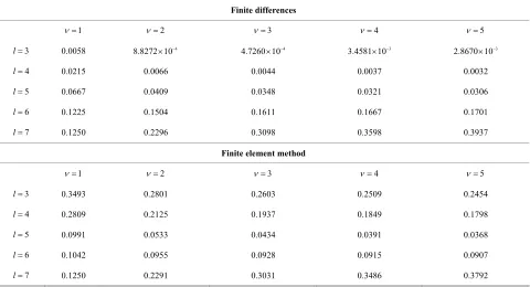
Table 1. The smoothig factor as a function of   12 and . l

Finite differences

1

 2 3 4 5

3

l 0.0058 _{8.8272 10}_ 4 _{4.7260 10}_ 4 _{3.4581 10}_ 3 _{2.8670 10}_ 3

4

l 0.0215 0.0066 0.0044 0.0037 0.0032

5

l 0.0667 0.0409 0.0348 0.0321 0.0306

6

l 0.1225 0.1504 0.1611 0.1667 0.1701

7

l 0.1250 0.2296 0.3098 0.3598 0.3937

Finite element method

1

 2 3 4 5

3

l 0.3493 0.2801 0.2603 0.2509 0.2454

4

l 0.2809 0.2125 0.1937 0.1849 0.1798

5

l 0.0991 0.0533 0.0434 0.0391 0.0368

6

l 0.1042 0.0955 0.0928 0.0915 0.0907

7

l 0.1250 0.2291 0.3031 0.3486 0.3792

(6)

 the Gauss-Seidel red-black relaxation method is a very good smoother for this problem as the smoothing factors in the cases presented here are 0.5;

 both the discretization methods lead to good smooth-ing factors. The finite element method seems slightly more appropriate when the number of grids used in the multigrid method is bigger;

 the number of relaxation steps before and after the coarse grid correction should not be too big as the smoothing factor increases with .

4.2. Asimptotic Convergence Factor and Error Reduction Factor

For the multigrid method having the components de-scribed in (9-16), the matrix of the two-grid operator for the problem (1) is:

 

_{ }





  



 





  



 

2

1 2

2

2 2

1 0 1

ˆ ˆ

0 1 4 2

1 cos 1 cos

ˆ

1 cos 1 cos

h

h h

h

h h

h

h h

M S

L

L L

S

L L





   



   

  

 _ _

  



 



 

 





 _ _ 

 



 

(26)

For π π, 2 2

 _ _

  the corresponding asimptotic

con-vergence factor and error reduction factor have been computed from the matrix (26) and are given in Table 2

for different numbers of pre- and post- smoothing steps. The data from Table 2 show that the multigrid method is very rapidly convergent: if at least one smoothing step is performed before and after the coarse grid correction, then the error is reduced by at least a factor per multigrid cycle.

3

10

5. Numerical Results

The problem (1) has been solved on a domain containing tree layers with different diffusion and convection coef-ficients ([16,17]).

The error was computed for the exact solution

 



 











2 3

, , max , 1.44 10 ,

0,1620 nm , 0, 24 min

ex

u x t x t ue x t

x t

   

   

The time step in the discretization process has been

dt60 s. Figure 1, Figure 2 and the Table 3 represent

[image:6.595.56.538.399.709.2]

the error after eight multigrid cycles, with two smoothing steps before and two after the coarse grid correction.

Table 2. Asimptotic convergence factor and error reduction factor



l6 .



Finite differences Finite element method

Number of

smoothig steps



2h



loc Mh





2h



loc Mh





2h



loc Mh





2h



loc Mh



1 0, 2 1

    0.1224 0.1731 0.0153 0.1989

1 1, 2 0

    0.1224 0.3297 0.0153 0.2420

1 1, 2 1

    0.0225 0.0570 _{9.1275 10}_ 4 _0.0037

1 2, 2 1

    0.0041 0.0105 _{6.8022 10}_ 5 _{2.5397 10}_ 4

1 2, 2 2

    _{7.5569 10}_ 4 _0.0019 _{5.6099 10}_ 6 _{2.0141 10}_ 5

1 3, 2 2

    _{1.3862 10}_ 4 _{3.5209 10}_ 4 _{4.8333 10}_ 7 _{1.7152 10}_ 6

(a) (b)

Figure 1. The multigrid error at ad = 100 nm in the skin for v1 = 1.0 × 10−10, v2 = 1.0 × 10−7, v3 = 1.0 × 10−7, d1 = 1 × 10−12, d2 = 1

−10 −10 4

(7)

[image:7.595.65.535.81.282.2]

(a) (b)

[image:7.595.58.285.333.576.2]

Figure 2. The multigrid err 1 2 3 10−6, d1 = 1 × 10−12, d2 = 1

Table 3. Multigrid error for FD and FEM. FD

or at ad = 100 nm in the skin for v = 1.0 × 10−9, v = 1.0 × 10−6, v = 1.0 × × 10−10_,_d

3 = 3 × 10−10; c = 103; a = 0.

   

maxiu xi uex xi uuex

3

l _{1.0000 10}_ 8 _{4.8970 10}_ 8

4

l _{1.0057 10}_ 8 _{3.1812 10}_ 8

5

l _{1.0617 10}_ 7 _{1.6775 10}_ 7

6

l _{8.3356 10}_ 7 _{1.9383 10}_ 6

7

l _{5.5076 10}_ 6 _{1.4308 10}_ 5

FEM

   

maxiu xi uex xi uuex

3

l _{9.9847 10}_ 9 _{4.7554 10}_ 8

4

l _{1.6648 10}_ 8 _{5.9871 10}_ 8

5

l 0.1079 0.2457

13.353

104.08 6

l 5 30.8845

7

l 64 245.1033

Table 3 shows the maximum absolute value of th er

a convergence and error analysis for

The convergence analysis showed that the discretization

[1] K. W. Morton merical Solution of Partial Differ troduction,” Cam-

e ror and the norm of the error vector corresponding to

Figures 1(a) and (b), for the finite differences discretization method (FD) and finite element method (FEM).

6. Conclusion

We have presented

the multigrid method applied to a time dependent diffusion-convection problem that is convection dominated. The mathematical model is applied to the study of the concentration of a solute that is transported by the blood, or the penetration of a substance through the skin layers.

process is better realized by the finite element method than the finite differences. Also the red-black Gauss- Seidel is a good smoother for the problem presented here, and needs not to be applied more than two or three times in the construction of the multigrid method.The numerical results in the previous paragraph confirmed the good convergence and error reduction as predicted by the coefficients computed with the local Fourier analysis.

REFERENCES

and D. F. Mayers, “Nu ential Equations, An In bridge University Press, Cambridge, 2005.

doi:10.1017/CBO9780511812248

[2] E. Becker, G. Carey and J. Oden, “Finite Introduction,” Prentice-Hall, Engle

Elements. An wood Cliffs, 1981.

ity

tions,” USSR Computational Mathe-

Process,” USSR Computational Mathematics and

ol. 31, [3] H. C. Elman, D. J. Silvester and A. J. Wathen, “Finite

Elements and Fast Iterative Solvers,” Oxford Univers Press, Oxford, 2005.

[4] R. P. Fedorenko, “A Relaxation Method for Solving El- liptic Difference Equa

matics and Mathematical Physics, Vol. 1, 1962, pp. 1092-

1096.

[5] R. P. Fedorenko, “The Speed of Convergence of One It- erative

Mathematical Physics, Vol. 4, 1964, pp. 227-235. [6] A. Brandt, “Multilevel Adaptive Solutions to Boundary

Value Problems,” Mathematics of Computation, V

1977, pp. 333-390.

doi:10.1090/S0025-5718-1977-0431719-X

[7] A. Brandt, “Multigrid Techniques: 1984 Guid

plications to Fluid Dynamics,” GMD-Studien Nr. 85, e with Ap- Augustin, Bonn, 1984.

(8)

[8] W. Hackbush,“Elliptic Differential Equations,” Springer- Verlag, New York, 1992.

doi:10.1007/978-3-642-11490-8

ondon, 2001.

rid Method,” obust Multigrid

nvection-Diffusion Equations,” Numerische

Ma-[9] U. Trottenberg, C. Oosterlee and A. Schuller, “Multigrid,” Elsevier Academic Press, L

[10] P. Weseling, “An Introduction to Multig John Wiley & Sons, New York, 1991. [11] M. A. Olshanski and A. Reusken, “On a R

Method for Connection-Diffusion Finite Element Prob- lems.”

http://www.math.uh.edu/ molshan/ftp/pub/proceed_cd.pdf [12] A. Reusken, “Convergence Analysis of a Multigrid Meth-

od for Co

thematik, Vol. 91, No. 2, 2002, pp. 323-349.

doi:10.1007/s002110100312

[13] R. Wienands and W. Joppich, “Practical Fourier Analysis for Multigrid Methods,” Chapman& Hall/CRC Press, Bo-

Element Method for Heat and ca Raton, 2005.

[14] R. W. Lewis, P. Nithiarasu and K. N. Seetharamu, “Fun- damentals of the Finite

Fluid Flow,” John Wiley & Sons Ltd, The Atrium, 2004.

doi:10.1002/0470014164

[15] W. L. Briggs, V. E. Henson and S. McCormick, “A Mul- tigrid Tutorial,”2nd Edition, Siam, Philadelphia, 2000.

doi:10.1137/1.9780898719505

[16] D. Neumann, “Modeling Transdermal Absorption,” Bi technology: Pharmaceutical Asp

o-ects, Springer, New York,

Transdermal Delivery of High Molecular Weight 2008.

[17] B. Al-Qallaf, D. Bhusan Das, D. Mori and Z. Cui,“Mod- elling

Drugs from Microneedle Systems,” Philosophical Trans- actions of the Royal Society A, Vol. 365, 2007, pp. 2951-