ISSN: 1816-949X
© Medwell Journals, 2020
θ3
L3
L1
θ1
θ2 L2
Simulation 3-DOF RRR Robotic Manipulator under PID Controller
Kamal M.H. Raheem and Ameer Najm Najaf
Department of Computer Engineering Technique, Engineering College,
Alkafeel University, Al-Najaf, Iraq
Abstract: A robotics manipulator system is a multi-link mechanical system each link is driven by an electrical actuator individually. Most industry application uses robotics system, this system needs to be controlled efficiently. In this study, 3-DOF serial robotic manipulator is simulated with a PID controller by using MATLAB\Simulink. The PID controller is proposed for every single manipulator where each manipulator is controlled independently. The performance of the 3-DOF robotic arm for trajectory tracking studies under this controller with different trajectory and without/with external disturbance torque.
Key words: Robot arm, robotics manipulator, 3-DOF, PID, MIMO PID controller, torque INTRODUCTION
Robotics manipulator can be classified in many categories such as application, type of link connection, number of Degree of Freedom (DOF), type of link motion and shape of the workspace and so on.
The 3-DOF serial (RRR) robotics manipulator can be used in many industry process like pick and place and painting. Various kind of robotic arms are designed according to the type of movement but the controller design is very important as mechanical part design. Many researches are available in the related literature to design controllers like PD or PID (Yamacli and Canbolat, 2008), neural network (Horowitz et al., 1991), fuzzy logic algorithm (Lewis et al., 1993) and artificial intelligence (Golnazarian, 1995; Jungbeck and Madrid, 2001).
In this study, a 3-DOF serial RRR robotics arm under its controller is simulated by using MATLAB/Simulink then the performance of controlled robot with adaptive PID controller will be discussed.
MATERIALS AND METHODS
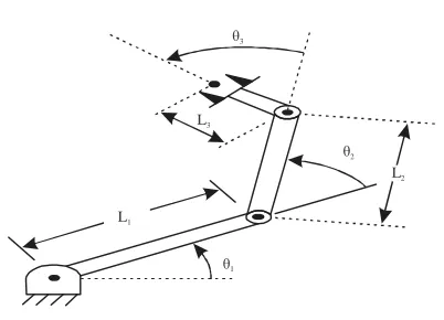
Configuration of 3-DOF robotics arm: The configuration of the serial 3-DOF robotics manipulator is shown in Fig. 1.
To find the kinematic equation of the manipulator, the Denative Hartenberg (DH) notation (Craig, 2005; Corke, 2007; Wang et al., 2014) will be used. The parameters of 3R robotics arm is shown in the Table 1. The transformation matrix for each link will be (Guo et al., 2015; Lloyd and Hayward, 1988):
(1) 1 1
1 1 0
1
C -S 0 0
S C 0 0
T =
0 0 1 0
0 0 0 1
[image:1.612.323.524.289.434.2]
Fig. 1: 3-DOF RRR robotics arm
Table 1: DH parameters for 3R robotics arm
i αi-1 ai-1 di θi
1 0 0 0 θ1
2 0 L1 0 θ2
3 0 L2 0 θ3
4 0 L3 0 0
(2)
2 2 1
2 1
2
C -S 0 L
S2 C 0 0
T =
0 0 1 0
0 0 0 1
(3)
3 3 2
3 3 3
2
C -S 0 L
S C 0 0
T =
0 0 1 0
0 0 0 1
(4) 3
3 4
1 0 0 L
0 1 0 0
T =
0 0 1 0
0 0 0 1
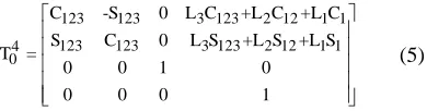
The transformation matrix of the end effector relative to the base will be (Liu et al., 2017; Cui et al., 2010):
(5) 123 123 3 123 2 12 1 1
123 123 3 123 2 12 1 1 4
0
C -S 0 L C +L C +L C
S C 0 L S +L S +L S
T =
0 0 1 0
0 0 0 1
The Lagrangian dynamic formulation (White et al., 1989; Yu et al., 2015) provides a means of deriving the equations of motion from a scalar function called the Lagrangian which is defined as the difference between the kinetic and potential energy of a mechanical system. The Lagrangian of a manipulator is:
(6)
E , = k , -u (7)
2
c
1 k , = m v* ,
2
The equations of motion for the manipulator are then given by:
(8) i
i i
E E
= -
where, r is the n×1 vector of actuator torques:
(9) i
i i i
d k k u
= - +
dt
(10)
= M +V , +G
Where:
M(θ) : Then 3×3 mass matrix of the manipulator : 3×1 vector of centrifugal and Coriolis terms V( , )
G(θ) : 3×1 vector of gravity terms
The term state-space equation will be used because the term V( , ) appearing in Eq. 10 has both position and velocity dependence (Guo et al., 2015).
Each element of M(θ) and G(θ) is a complex function that depends on θ, the position of all the joints of the manipulator. Each element of V( , ) is a complex function of both θ and . Table 2 present the simulation parameters of the robot manipulator.
PID controller: Generally, a PID controller of each joint controlled independently is given with the formula (Goldman, 1983; Astrom and Hagglund, 1995;
[image:2.612.103.298.133.184.2]Han et al., 2014). The PID controller is most used in
Table 2: Robot parameters
Parameters Link 1 Link 2 Link 3
Mass (kg) 0.30 0.25 0.15
Length (m) 0.25 0.20 0.15 Moment of inertia (kgm2) 0.02 0.02 0.02
Table 3: Parameters of PID controllers
Variables Link 1 Link 2 Link 3
KP 18.00 18.5 19.50
KI 49.00 50.0 49.88
Kd 2.51 2.0 2.70
control system. The main and important advantage of PID controller is its feasibility and easy to be implemented. The main equation of PID controller is (Ang et al., 2005; Bingul, 2004; Allaoua et al., 2010; Wang et al., 2006):
(11)
i
i Pi i d i
i
de t 1
t = K e t +K + e t dt
dt K
Where:
e(t) : The error function
KP : The proportional control coefficient which
providing control proportional to the error Kd : The derivative control coefficient which used to
improve transient response
Ki : The integral control coefficient used to reduce the
steady state errors
The PID parameters are given as shown in Table 3. RESULTS AND DISCUSSION
Simulation models of 3-DOF robotics manipulator with PID controller and results: Dynamic of the 3-DOF robotics arm with PID controller simulated by MATLAB\Simulink Fig. 2. The response will be under PID controller with different desired angles and without/with disturbance.
Trajectory performance, torque performance and position error are discussed in PID controllers. Figure 3 and 4 shows the link angles and the link angle errors with PID controller, respectively for step trajectories and without disturbance.
Assume the external disturbance torques as shown in Fig. 5. Figure 6 shows the response of the all links when the external disturbance is applied.
So, the error in the position of all links of the robotics manipulator will be as Fig. 7. When the desired angle of the three links of the robotics arm is sine wave, the response of these links will be as Fig. 8.
Stop 2
M 11 M 12 M 13
Out 1 -Matrix 3×1
Scope 3
In 1Out 1 Subsystem
-Inv [A]
(3×3) Invert 3×3 matrix
Out1 L1 m1 m2 L2 2 m3 L3 3 l 1 l 2 1 3
0.02 0.02 0.02 L2 L1 Matrix multiply Product
Out 1 L1 m1 1 m2 L2 2 m3 L3 3 1 Dot 2 Dot 3 Dot C+G Out 1
M 11 M 12 M 13 Matrix 3×1
Scope
1/5 1/5
1/5 1/5
1/5 1/5
Integrator Integrator 3 Integrator 5 Integrator 2
Integrator 1 Integrator 4
Out 1 Out 2 Out 3 Out 4 Out 5 Out 6 Mass and lenght M Matrix3×3
L3
0 1 2 3 4 5 6 7 8 9 10 Time (sec)
2 1 0 -1 -2 -0
Di
st
u
rb
an
c
e t
o
rq
u
e
Time (sec) 1.0
0.5 0 -0.5 -1.0
0 5 10 15 20 25 30
An
g
le
s (
ra
d
)
Desired angles Angle of link 1
[image:3.612.77.530.89.729.2]Angle of link 2 Angle of link 3
Fig. 2 Simulink model of 3-DOF robotics arm
[image:3.612.93.510.93.337.2]Fig. 3: Link angles of 3-DOF robotics arm
Fig. 4: Link angles error of 3-DOF robotics arm
[image:3.612.81.272.372.465.2]Fig. 5: External disturbance torques
Fig. 6: Response of the all links when the external disturbance is applied
Fig. 7: Error in the position
Fig. 8: Response of all links for desired sine angles 1.2
1.0 0.8 0.6 0.4 0.2 0.0
A
ngl
e (Rad
)
0 0.2 0.4 0.6 0.8 1.0 1.2 1.4 1.6 1.8 2.0 Time (sec)
Onset = 0
Desired angles Output angle of link 1 Output angle of link 2 Output angle of link 3
1.4 1.2 1.0 0.8 0.6 0.4 0.2 0 -0.2
A
ngl
e (Rad
)
0 1 2 3 4 5 6 7 8 9 10 Time (sec)
Desired angles Output angle of link 1 Output angle of link 2 Output angle of link 3
1.2 1.0 0.8 0.6 0.4 0.2 0.0
Error of angle (Ra
d
)
0 0.2 0.4 0.6 0.8 1.0 1.2 1.4 1.6 1.8 2.0 Time (sec)
Error angle of link 1 Error angle of link 2 Error angle of link 3
1.2 1.0 0.8 0.6 0.4 0.2 0.0 -0.2 -0.4
Error of angle (Ra
d
)
0 1 2 3 4 5 6 7 8 9 10 Time (sec)
[image:3.612.83.281.616.704.2]0 5 10 15 20 25 30 Time (sec)
1.2 1.0 0.8 0.6 0.4 0.2 0.0 -0.2 -0.4 -0.6 -0.8
D
is
tu
rb
an
ce
t
o
rq
u
e
Fig. 9: Error of the trajectory
Fig. 10: External disturbance torques
Fig. 11: The response for sine wave desired angles with external disturbance
Fig. 12: Error of all links position with external disturbance
If the disturbance as Fig. 10 will be applied, the response of all three links will be as Fig. 11 and the error in angles of links will be as Fig. 12.
Figure 11 shows the response of these links when the desired angle of the three links of the robotics arm is sine wave. The error of all links position of the robotics manipulator after the external disturbance applied will be as Fig. 7.
Fig. 13: External disturbance torque with different desired angle
Fig. 14: Link angles with different desired angle and with external disturbance
Fig. 15: Error of link angles with different desired angle
Table 4: Maximum error response
Desired angle Max. disturbance Link 1 Link 2 Link 3 Unit step ……. 0.150 0.180 0.175 Unit step -2 to 2 0.19 0.220 0.210 Sinusoidal …… 0.035 0.025 0.013 Sinusoidal -0.75 to 1.1 0.075 0.075 0.075 Unit step+sinusoidal …… 0.120 0.140 0.130 Unit step+sinusoidal -2.5 to 2.5 0.170 0.190 0.170
Figure 13 shows the external disturbance when the desired angle of the first and third link as a unit step and the desired angle of the second link as sine wave angle, the response will be as shown in Fig. 14.
The error of the angle of links when the desired angles are different and with external disturbance will be as shown in Fig. 15.
The response for desired angles (unit step, sinusoidal, unit step and sinusoidal) represented with/without external disturbance torque. The maximum error of each link in each case is shown in Table 4.
CONCLUSION
The robotics manipulators became very important and used widely in industry, thus, the study and control of the joints is very vital. In this study, the 0.04
0.03 0.02 0.01 0.00 -0.01 -0.02 -0.03 -0.04
Error of angles (R
ad)
0 5 10 15 20 25 30 Time (sec)
Error of link 1 angle Error of link 2 angle
Error of link 3 angle
1.0 0.5 0.0 -0.5 -1.0
Error of angles (R
ad)
0 5 10 15 20 25 30 Time (sec)
Angle of link 2 Angle of link 3 Sine wave
Angle of link 1 1.0 0.8
0.6 0.4 0.2 0.0 -0.2
Error of angle link
s (Rad
)
0 5 10 15 Time (sec)
Error of link 1 Error of link 2 Error of link 3 1.0
0.5 0.0 -0.5 -1.0
A
ngl
e (Rad
)
0 5 10 15 Time (sec)
Unit step Angle of linke 1
Angle of linke 2 Angle of linke 3 2
1 0 -1 -2 -3
Di
stur
ba
nce
exter
n
al torque
0 5 10 15 Time (sec)
0.08 0.06 0.04 0.02 0.00 -0.02 -0.04 -0.06 -0.08
Error of an
g
le
(Ra
d
)
0 5 10 15 20 25 30 Time (sec)
Error angle of link 1 Error angle of link 2
analysis of 3-DOF robotic arm has done and the dynamic equations has been represented by using Lagrangian dynamic formulation. Beside the dynamic model has been simulated by using MATLAB/Simulink and controlled by PID controller. The response of all links of 3-DOF robotics manipulator under the PID controller is represented when the desired angles be: unit step, sinusoidal and unit step and sinusoidal.
REFERENCES
Allaoua, B., A. Laoufi and B. Gasbaoui, 2010. Multi-drive paper system control based on multi-input multi-output PID controller. Leonardo J. Sci., 9: 59-70.
Ang, K.H., G. Chong and Y. Li, 2005. PID control system analysis, design and technology. IEEE Trans. Control Systems Technol., 13: 569-576.
Astrom, K.J. and T. Hagglund, 1995. Pid Controllers: Theory, Design, and Tuning. 2nd Edn., International Society of Automation, North Carolina, USA., ISBN-13:978-1556175169, Pages: 343.
Bingul, Z., 2004. A new PID tuning technique using differential evolution for unstable and integrating processes with time delay. Proceedings of the International Conference on Neural Information Processing, November 22-25, 2014, Springer, Berlin, Germany, ISBN:978-3-540-23931-4, pp: 254-260.
Corke, P.I., 2007. A simple and systematic approach to assigning Denavit-Hartenberg parameters. IEEE. Trans. Rob., 23: 590-594.
Craig, J.J., 2005. Introduction to Robotics Mechanics and Control. 3rd Edn., Pearson Education Inc., New Jersey.
Cui, Y., P. Shi and J. Hua, 2010. Kinematics analysis and simulation of a 6-DOF humanoid robot manipulator. Proceedings of the 2010 2nd International Asia Conference on Informatics in Control, Automation and Robotics (CAR 2010) Vol. 2, March 6-7, 2010, IEEE, Wuhan, China, ISBN:978-1-4244-5192-0, pp: 246-249.
Goldman, R., 1983. Design of an interactive manipulator programming environment. Ph.D Thesis, Stanford University, Stanford, California.
Golnazarian, W., 1995. Time-varying neural networks for robot trajectory control. Ph.D Thesis, University of Cincinnati, Cincinnati, Ohio.
Guo, W., R. Li, C. Cao and Y. Gao, 2015. Kinematics analysis of a novel 5-DOF hybrid manipulator. Intl. J. Autom. Technol., 9: 765-774.
Han, J., X. Li and Q. Qin, 2014. Design of two-wheeled self-balancing robot based on sensor fusion algorithm. Intl. J. Autom. Technol., 8: 216-221. Horowitz, R., W. Messner and J.B. Moore, 1991.
Exponential convergence of a learning controller for robot manipulators. IEEE. Trans. Autom. Contr., 36: 890-894.
Jungbeck, M. and M.K. Madrid, 2001. Optimal neural network output feedback control for robot manipulators. Proceedings of the 2nd International Workshop on Robot Motion and Control RoMoCo’01 (IEEE Cat. No.01EX535), October 20, 2001, IEEE, Bukowy Dworek, Poland, Poland, ISBN:83-7143-515-0, pp: 85-90.
Lewis, F.L., C.T. Abdallah and D.M. Dawson, 1993. Control of Robot Manipulators. Macmillan Pub. Co., New York.
Liu, F., G. Gao, L. Shi and Y. Lv, 2017. Kinematic analysis and simulation of a 3-DOF robotic manipulator. Proceedings of the 2017 3rd International Conference on Computational Intelligence and Communication Technology (CICT), February 9-10, 2017, IEEE, Ghaziabad, India, ISBN:978-1-5090-6219-5, pp: 1-5.
Lloyd, J.E. and V. Hayward, 1988. Kinematics of common industrial robots. Robot. Auton. Syst., 4: 169-191.
Wang, H., H. Qi, M. Xu, Y. Tang and J. Yao et al., 2014. Research on the Relationship between classic Hartenberg and modified Denavit-Hartenberg. Proceedings of the 2014 7th International Symposium on Computational Intelligence and Design (ISCID) Vol. 2, December 13-14, 2014, IEEE, Hangzhou, China, ISBN:978-1-4799-7004-9, pp: 26-29.
Wang, J.S., Y. Zhang and W. Wang, 2006. Optimal design of PI/PD controller for non-minimum phase system. Trans. Instit. Measur. Contr., 28: 27-35. White, W.N., D.D. Niemann and P.M. Lynch, 1989. The
presentation of Lagrange’s equations in introductory robotics courses. IEEE. Trans. Educ., 32: 39-46. Yamacli, S. and H. Canbolat, 2008. Simulation of a
SCARA robot with PD and learning controllers. Simul. Modell. Pract. Theor., 16: 1477-1487. Yu, Y., P. Qi, K. Althoefer and H.K. Lam, 2015.