Construction and sharp consistency estimates for atomistic/continuum coupling methods with general interfaces : a two dimensional model problem

http://wrap.warwick.ac.uk/

Original citation:

Ortner, Christoph and Zhang, L. (2012) Construction and sharp consistency estimates

for atomistic/continuum coupling methods with general interfaces : a two-dimensional

model problem. SIAM Journal on Numerical Analysis, Volume 50 (Number 6). pp.

2940-2965.

Permanent WRAP url:

http://wrap.warwick.ac.uk/60457

Copyright and reuse:

The Warwick Research Archive Portal (WRAP) makes this work of researchers of the

University of Warwick available open access under the following conditions. Copyright ©

and all moral rights to the version of the paper presented here belong to the individual

author(s) and/or other copyright owners. To the extent reasonable and practicable the

material made available in WRAP has been checked for eligibility before being made

available.

Copies of full items can be used for personal research or study, educational, or

not-for-profit purposes without prior permission or charge. Provided that the authors, title and

full bibliographic details are credited, a hyperlink and/or URL is given for the original

metadata page and the content is not changed in any way.

Publisher’s statement:

© SIAM

http://dx.doi.org/10.1137/110851791

A note on versions:

The version presented here may differ from the published version or, version of record, if

you wish to cite this item you are advised to consult the publisher’s version. Please see

the ‘permanent WRAP url’ above for details on accessing the published version and note

that access may require a subscription.

ATOMISTIC/CONTINUUM COUPLING METHODS WITH

GENERAL INTERFACES: A 2D MODEL PROBLEM∗

C. ORTNER† ANDL. ZHANG‡

Abstract. We present a new variant of the geometry reconstruction approach for the formu-lation of atomistic/continuum coupling methods (a/c methods). For many-body nearest-neighbour interactions on the 2D triangular lattice, we show that patch test consistent a/c methods can be constructed for arbitrary interface geometries. Moreover, we prove that all methods within this class are first-order consistent at the atomistic/continuum interface and second-order consistent in the interior of the continuum region.

Key words. atomistic models, quasicontinuum method, coarse graining

AMS subject classifications. 65N12, 65N15, 70C20

1. Introduction. Atomistic/continuum coupling methods (a/c methods) are a class of coarse-graining techniques for the efficient simulation of atomistic systems with localized regions of interest interacting with long-range elastic effects that can be adequately described by a continuum model. We refer to [7], and references therein, for an introduction and discussion of applications.

In the present work we are concerned with the construction and rigorous analysis of energy-based a/c methods in a 2D model problem. Our starting point is the geometry reconstruction approach proposed by Shimokawa et al [18] and by E, Lu and Yang [4] for the construction of “consistent” a/c methods in 2D and 3D. We propose a new variant of that approach to define a modified site potential at the a/c interface, which has several free parameters. We then “fit” these parameters so that the resulting a/c hybrid energy satisfies an energy consistency condition and a force consistency condition (see (2.6) and (2.7) for the precise definition of these terms; in the terminology of quasicontinuum methods our hybrid energy is free of ghost forces). Explicit constructions along these lines can be found in [18] for pair potentials and in [4] for coupling a finite-range many-body potential to a nearest-neighbour potential, for high-symmetry interfaces. Our focus in the present work is the coupling to a continuum model and interfaces with corners; both of these cases are only briefly touched upon in [4].

In recent years there has been considerable activity in the numerical analysis literature on the classification and rigorous analysis of a/c methods (see [2, 3, 8, 11, 13] and references therein). Much of this work has been restricted to one-dimensional problems; only very recently some progress has been made on the analysis of a/c methods in 2D and 3D [6, 10, 12].

The first rigorous error estimates for the method proposed in [4] (together with a wider class of related methods), in more than one dimension, are presented in [10] for

∗_{This work was supported by EPSRC Grant “Analysis of Atomistic-to-Continuum Coupling}

Meth-ods” and the EPSRC Critical Mass Programme “New Frontiers in the Mathematics of Solids” (Ox-MoS).

†_{Mathematics Institute, Zeeman Building, University of Warwick, Coventry, CV4 7AL, UK}

([email protected]).

‡_{Department of Mathematics, Institute of Natural Sciences, and Ministry of Education Key}

Labo-ratory of Scientific and Engineering Computing (MOE-LSC), Shanghai Jiao Tong University, Shang-hai 20040, China, ([email protected]).

2D finite range many-body interactions. The work [10] assumesthe existence of an interface potential so that the resulting a/c energy satisfies certain energy and force consistency conditions (a variant of the patch test) and then established first-order consistency of the resulting a/c method in negative Sobolev norms.

Several important questions remain open: 1. It is yet unclear whether construc-tions of the type proposed in [4, 18] can be carried out for interfaces with corners. 2. The error estimates in [10] contain certain non-local terms that enforce unnatural as-sumptions (e.g., connectedness of the atomistic region). 3. Moreover, this nonlocality causes suboptimal error estimates; namely, it destroys the second-order consistency of the Cauchy–Born model (see, e.g., [2, 5, 11]), and an unnatural dependence of the interface width enters the error estimates. (Moreover, we note that the error estimates in [12] for a different a/c method are only first-order as well.)

The purpose of the present work is to investigate for a model problem whether these restrictions are genuine, or of a technical nature. To that end we formulate an atomistic model on the 2D triangular lattice with nearest-neighbour many-body interactions (effectively these are third neighbour interactions), and construct new a/c methods in the spirit of [4, 18]. We then prove that the resulting methods are all first-order consistent in the interface region and second-first-order consistent in the interior of the continuum region, which is the first generalisation of the optimal one-dimensional result [11, Theorem 3.1] to two dimensions.

Although it may seem restrictive at first glance to consider only nearest-neighbour potentials, we note that this is in fact an important case to consider. For example, bond-angle potentials (which are included in our analysis) usually consider only angles between nearest-neighbour bonds. More generally, many-body effects are usually restricted to very small interaction neighbourhoods, while long-range effects are often only displayed in pair potentials (in particular, Lennard-Jones), which can be treated, for example, using Shapeev’s method [12, 16, 15].

2. Atomistic/Continuum Coupling.

2.1. Atomistic model. We consider a nominally infinite crystal, but restrict admissible displacements to those with compact support. Thus we avoid any discus-sion of boundary conditions, which are unimportant for the purpose of this work.

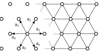
LetQ6denote a rotation through arclengthπ/3. As a reference configuration we

choose the triangular lattice (see also Figure 2.1):

L:=AZ2, where A:= (a1, a2),

a1:= (1,0)>, andaj :=Q j−1

6 a1, j∈Z.

We will frequently use the following relationships between the vectorsaj:

aj+6=aj, aj+3=−aj, and aj−1+aj+1=aj for allj∈Z.

For future reference we also definea:= (aj)6j=1, andFa:= (Faj)6j=1, forF∈R2×2.

Our choice of reference configuration is largely motivated by the fact that L possesses a canonical triangulation (see Figure 2.1, and§2.2), which will be convenient in our analysis.

The set of displacements and deformations with compact support are given, re-spectively, by

U0: = u:L →R2:u(x)6= 0 for at most finitely manyx∈ L , and

Y0: =

Fig. 2.1. The 2D triangular lattice and its canonical triangulation.

We remark that deformations are usually required to be at least invertible, but that we avoid this requirement by making simplifying assumptions on the interaction po-tential.

A homogeneous deformation is a mapyF:L →R2,yF(x) :=Fx, whereF∈R2×2.

We note thatyF∈/Y0unlessF=I.

For a mapv:L →R2, we define the forward finite difference operator

Djv(x) :=v(x+aj)−v(x), x∈ L, j∈Z,

and the family of all nearest-neighbour finite differences,Dy(x) := (Djy(x))6j=1.

We assume that the atomistic interaction is described by a nearest-neighbour many-body site energy potentialV ∈C3(R2×6), withV(a) = 0, so that the energy of

a deformationy∈Y0is given by

Ea(y) := X

x∈L

V Dy(x) .

This is the most general form of nearest-neighbour interactions in the 2D triangular lattice.

The assumptionV(a) = 0 guarantees thatEa(y) is finite for ally∈Y0.

2.2. The Cauchy–Born approximation. For fields y ∈ W1,∞₍

R2;R2), such

thaty−id has compact support, we define the Cauchy–Born energy functional

Ec(y) := Z

R2

W(∂y) dx, where W(F) := _Ω1

0V Fa

,

W ∈C3(R2×2;R), is theCauchy–Born stored energy function. The factor Ω0:=

√ 3/2 is the volume of one primitive cell ofL, that is, W(F) is the energy per unit volume of the homogeneous latticeFL.

Ify∈Y0is adiscretedeformation, then we define its Cauchy–Born energy through

piecewise affine interpolation: The triangular lattice Lhas a canonical triangulation T into closed triangles depicted in Figure 2.1. Henceforth, we shall always identify a functionv :L →Rk with its P1-interpolant, which belongs to W1,∞(R2;Rk). For a

discrete deformationy∈_Y0, we can then write the Cauchy–Born energy as

Ec(y) = Z

R2

W(∂y) dx= X T∈T

|T|W(∂Ty), (2.1)

where we define∂Ty:=∂y(x)|x∈T and note that|T|= Ω0/2 for all trianglesT ∈T.

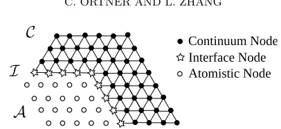
Atomistic Node Interface Node Continuum Node

Fig. 2.2.Atomistic-interface-continuum domain decomposition.

Alternatively,Ec can be written in terms of site energies, which will be helpful for

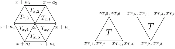
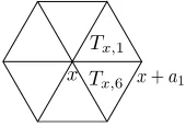
the definition of a/c methods. Each vertexx∈ Lhas six adjacent triangles, which we denote by Tx,j := conv{x, x+aj, x+aj+1}, j = 1, . . . ,6 (cf. Figure 2.3). With this

notation,

Ec(y) = X

x∈L

Vc(Dy(x)), where Vc(Dy(x)) := Ω0 6

6 X

j=1

W(∂Tx,jy). (2.2)

Note that Vc ∈ C3(R2×6) is well-defined since ∂Tx,jy is determined by the finite

differencesDjy(x) andDj+1y(x).

2.3. A/c coupling via geometry reconstruction. LetA ⊂ Ldenote the set of all lattice sites for which we require full atomistic accuracy. We denote the set of interface lattice sites by

I :=x∈ L \ A

x+aj ∈ Afor somej∈ {1, . . . ,6} ,

and we denote the remaining lattice sites byC:=L \(A ∪ I); cf. Figure 2.2. We note that we have a single layer of interface atoms where we can modify the interaction law to obtain a “consistent” a/c coupling energy. In general, the interface region has to be widened according to the interaction range [4].

A general form for the constuction of a/c coupling energies is

Eac(y) = X

x∈A

V(Dy(x)) +X x∈I

V_xi(Dy(x)) +X x∈C

Vc(Dy(x)), (2.3)

where Vi

x, x∈ I, are the interface site potentials that define the method (the atom-istic site potential and the continuum site potential are determined by the atomatom-istic model).

For example, if we choose Vxi =V, then we obtain the original quasicontinuum

method[9] (the QCE method). It is well understood that the QCE method suffers from

the occurance of ghost forces, which result in large modelling errors [2, 7, 8, 13, 17]. In the following we present a new variant of the geometry reconstruction approach [4, 18] for constructingVi_{. We define the interface potential as}

V_xi(Dy(x)) :=V(RxDy(x)), (2.4)

whereRxis a geometry reconstruction operatorof the general form

RxDy(x) := RxDjy(x)

6

j=1, and RxDjy(x) := 6 X

i=1

Here (Cx,j,i)6j,i=1, x∈ I, are free parameters of the method that can be determined

to improve the accuracy of the coupling scheme.

Remark 2.1. There is no choice of the reconstruction operatorRxso thatVi is

equal to Vc_{, whereasV}a _{can be written in the form (2.4)by takingC}

x,j,i=δij.

We use the acronym “GR-AC method” (geometry reconstruction-based atomistic-to-continuum coupling method) to describe methods of the type (2.3) where the in-terface site potential is of the form (2.4).

We aim to determine parametersCx,j,isuch that the coupling energyEacsatisfies

the followinglocal energy consistencyandlocal force consistencyconditions:

Vxi(Fa) =V(Fa) ∀F∈R2×2, ∀x∈ I, and (2.6)

fac(x;yF) = 0 ∀F∈R2×2, ∀x∈ L, (2.7)

wherefac(x;y) is the force acting on the atom at sitex, initially defined by

fac(x;y) :=− ∂Eac(y)

∂y(x) ∈R

2 _fory

∈Y0;

however, we immediately see that fac involves only a sum over a finite set of lattice

sites, and hence the formula can be extended to all mapsy :L →_R2_{. In particular,}

(2.7) is a well-posed condition. Taken together, we call (2.6) and (2.7) thepatch test. A hybrid energyEacof the form (2.3) is calledpatch test consistentif it satisfies both

conditions.

In the remainder of the paper, we will determine choices of the parametersCx,j,i for general a/c interface geometries that give patch test consistent coupling methods. Moreover, we will prove that for all parameter choices we determine, the resulting a/c method is first-order consistent at the interface and second-order consistent in the interior of the continuum region. This extends the optimal 1D result in [11].

Remark 2.2. 1. To obtain a method with improved complexity one should use a coarser finite element discretisation in the continuum region. If coarsening is included

in the a/c method, then the consistency analysis involves estimating the coarsening

erroras well as the modelling error.

It was seen in [13, 10] that the coarsening step can be understood using standard finite element methodology, and hence we focus only on the modification of the model, and the resulting modelling errors. Since the coarsening error is ignored, we will use the terms modelling errorandconsistency error interchangably.

2. Realistic interaction potentials have singularities for colliding nuclei, i.e., for deformations that are not injective. Clearly, our assumption that V ∈C3₍

R2×6) con-tradicts this. It is conceptually easy to admit more general site potentials in our work, however, this would introduce additional technical steps that are of little relevance to the problems we wish to study.

2.4. Additional assumptions and notation. We use|·|to denote the`2-norm on _Rn_{, and the Frobenius norm on}

Rn×m. Generic constants that are independent

2.4.1. Properties of V. We define notation for partial derivatives of V, for

g∈R2×6, as follows:

∂jV(g) :=

∂V(g)

∂gj

∈_R2_{, and ∂}

i,jV(g) :=

∂2_V(g) ∂gi∂gj

∈_R2×2_{, fori, j∈ {1, . . . ,6},}

and similarly, the third derivative ∂i,j,kV(g)∈R2×2×2, which we will never use

ex-plicitly.

Interpreting the second and third partial derivatives as multi-linear forms we define the global bounds

M2:=

6 X

i,j=1

sup

g∈R2×6

sup h1,h2∈R2 |h1|=|h2|=1

∂i,jV(g)[h1, h2], and

M3:= 6 X

i,j,k=1

sup

g∈R2×6

sup h1,h2,h3∈R2

|h1|=|h2|=|h3|=1

∂i,j,kV(g)[h1, h2, h3].

Remark 2.3. For realistic interaction potentials, the energy of colliding nuclei is infinite. Similarly, it is sometimes convenient to use interaction potentials that grow superlinearly at infinite. In either of these cases, we would obtainM2=M3=∞.

To avoid this difficulty, we could simply restrictgin the definition ofM2, M3 to

a neighbourhood of the range of Dy(x)of an appropriate range of deformations y of interest.

With this notation it is straightforward to show that

6 X

i=1

∂iV(g)−∂iV(h)

≤M2 max

j=1,...,6|gj−hj|, forg,h∈R

2×6_{. (2.8)}

We also assume thatV satisfies the point symmetry

V (−gj+3)6j=1

=V(g) ∀g∈R2×6. (2.9)

The following identities are immediate consequences of this condition:

∂iV(Fa) = −∂i+3V(Fa), fori= 1, . . . ,6, F∈R2×2 (2.10)

∂ijV(Fa) = ∂i+3,j+3V(Fa), fori, j= 1, . . . ,6, F∈R2×2. (2.11)

We will prove results on the classV, of all site potentials that satisfy (2.9),

V :=

V ∈C3(R2×6) V satisfies (2.9) .

We will frequently use the following shorthand notation for partial derivatives of

V, when there is no ambiguity in their meaning:

Vx,j :=∂jV(Dy(x)), VF,j :=∂jV(Fa), VT ,j:=V∂Ty,j,

Fig. 2.3.Convention for the symbolsTx,j andxT ,j.

2.4.2. Linear functionals. For y ∈Y0 and u∈U0 we denote the directional

derivative ofEa by

δEa(y), u:= lim

t→0

Ea(y+tu)−Ea(y)

t .

We callδEa(y) thefirst variation of Ea and understand it as an element of U0∗. We

use analogous notation for other functionals. This paper is largely concerned with establishing bounds on themodelling errorδEa(y)−δEac(y).

To obtain sharp error estimates in W1,p_{-like norms, one needs to bound modelling} errors in negative Sobolev norms, or, in our case, discrete versions thereof. Let ` : U0→Rbe a linear functional, and let 1p+

1

p0 = 1, 1≤p, p0 ≤ ∞, then we define

k`k_U−1,p := sup

u∈U0

k∂uk

Lp0=1

`, u.

2.4.3. Notation for the lattice and the triangulation. L is the set of ver-tices of T, and we denote the set of edges of T by F, with edge midpoints mf,

f ∈F.

For each vertexx∈ Land directionaj, letTx,j := conv{x, x+aj, x+aj+1} ∈T, j = 1, . . . ,6 (see Figure 2.3). The edge (x, x+aj) is the intersection of the two elementsTx,j andTx,j−1. Moreover, let xT ,j ∈ Lbe the unique lattice point so that bothxT ,j, xT ,j+aj∈T (again, see Figure 2.3).

2.4.4. Discrete regularity. To measure regularity or “smoothness” of discrete deformationsy∈Y0, we first define the symbols

|D2y(x)|:= max

i,j=1,...,6|DiDjy(x)|, and |D

3_{y(x)|:= max}

i,j,k=1,...,6|DiDjDky(x)|,

forx∈ L. With mild abuse of notation, we then define the norms

kD2yk`p(A):=k|D2y|k`p(A), and kD3yk`p(A):=k|D3y|k`p(A),

for anyA ⊂ Landy∈Y0. If the labelAis omitted, then it is assumed thatA=L.

3. Construction of the GR-AC Method. In this section we carry out an

We assume throughout the remainder of the paper that the reconstructed differ-ence RxDjy(x) may depend only on the original differences Dj−1y(x), Djy(x), and

Dj+1y(x), that is,

Cx,j,i= 0 for

(i−j) mod 6

>1, i, j∈ {1, . . . ,6}, x∈ I. (3.1)

For future reference, we call (3.1) theone-sidedness condition.

In§3.1 and§3.2 we derive general conditions on the parameters that are indepen-dent of the choice of the atomistic region. In§3.3 and§3.4 we then compute explicit sets of parameters.

3.1. Conditions for local energy consistency. We first derive conditions for the local energy consistency condition (2.6).

Proposition 3.1. Suppose that the parameters Cx,j,i satisfy the one-sidedness

condition (3.1), then the interface potential Vi

x satisfies the local energy consistency

condition (2.6) for all potentialsV ∈V if and only if

Cx,j,j−1=Cx,j,j+1= 1−Cx,j,j, forj= 1, . . . ,6. (3.2)

Proof. We require thatVi

x(Fa) =V(Fa), for arbitraryV ∈V, which is equivalent to

Faj=

6 X

i=1

Cx,j,iFai forj= 1, . . . ,6.

Since this has to hold for arbitrary F∈ R2×2, and in view of (3.1), we obtain the

condition

aj=Cx,j,j−1aj−1+Cx,j,jaj+Cx,j,j+1aj+1

Sinceaj=aj−1+aj+1, this is equivalent to

(Cx,j,j−1+Cx,j,j−1)aj−1+ (Cx,j,j+1+Cx,j,j−1)aj+1= 0,

and sinceaj−1, aj+1 are linearly independent, we obtain the condition that

Cx,j,j−1+Cx,j,j= 1, and Cx,j,j+1+Cx,j,j= 1.

Subtracting these two conditions givesCx,j,j+1=Cx,j,j−1, and hence we obtain (3.2).

As a consequence of Assumption (3.1), and Proposition 3.1, we have reduced the number of free parameters to six for each site x ∈ I. To simplify the subsequent notation, whenever the parametersCx,j,i are chosen to satisfy (3.2), we will write

Cx,j :=Cx,j,j, and note thatCx,j,j−1=Cx,j,j+1= 1−Cx,j. (3.3)

3.2. Conditions for local force consistency. We rewrite Eac in terms of a

hybrid site potential

Eac(y) = X

x∈L

V_xac(Dy(x)), where V_xac(g) :=

 



Vc_{(g), x∈ C,} Vi

x(g), x∈ I,

V(g), x∈ A.

(3.4)

Although there exists no reconstruction opertorRsuch thatVc=V(R(Dy)) for arbitary deformationy(see Remark 2.1), it can be shown by direct calculation that, if we take the coefficients of reconstruction operatorRasCx,j := 2/3, thenV(R(Dy)) andVc _{produce same forces for homogenenous deformationy}

F. Therefore, to enforce

the local force consistency condition, we can assign values of coefficients to atoms in the atomistic and continuum domain such that

Cx,j := 1 forx∈ A and Cx,j := 2/3 forx∈ C, j= 1, . . . ,6, (3.5)

and these coefficents are compatible with (3.1) and (3.3) as well.

Lemma 3.2. Suppose that the parameters (Cx,j,i)6i,j=1, x ∈ I, satisfy the

one-sidedness condition (3.1)and local energy consistency (3.3), then

−fac(x;yF) = 6 X

j=1 6 X

i=1

(Cx−ai,j,i−Cx,j,i)VF,j ∀x∈ L. (3.6)

(3.6)is well-defined if we take values of Cx,j,i from (3.5)whenx∈ A ∪ C.

Proof. Using the notation (3.4), we have

hδEac(yF), ui= X

x∈L

6 X

i=1

∂iVxac(Fa)·Diu(x),

which immediately gives

−fac(x;yF) = 6 X

i=1

∂iVxac−ai(Fa)−∂iV

ac

x (Fa)

. (3.7)

With the notation introduced in (3.5), we obtain

6 X

i=1

∂iVxac(Fa)·Diu(x) =

6 X

j=1 VF,j

6 X

i=1

Cx,j,iDiu(x),

which implies

∂iVxac(Fa) =

6 X

j=1

Cx,j,iVF,j. (3.8)

Combining (3.8) with (3.7) yields (3.6).

Testing (3.6) for allV ∈V andF∈_R2×2_{, we obtain the next result.}

Lemma 3.3. Suppose that the parameters(Cx,j,i)6i,j=1, x∈ I, satisfy one-sidedness

(3.1)and local energy consistency(3.2). ThenEacsatisfies local force consistency(2.7)

for allV ∈V if and only if

6 X

i=1

Cx−ai,j,i−Cx−ai,j+3,i−Cx,j,i+Cx,j+3,i

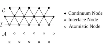
Fig. 3.1.The flat interface case.

Proof. Using (3.6) and point symmetry (2.10) one readily checks that (3.9) is

sufficient for force consistency (2.7). To show that (3.9) is also necessary we test (3.6) with

V(g) =1₂ |g1−a1|2_+|g4−a4|2 ,

which clearly belongs to the classV, to obtain

−fac(x;yF) = X

j=1,4 6 X

i=1

(Cx−ai,j,i−Cx,j,i)(F−I)aj

=

6 X

i=1

Cx−ai,1,i−Cx−ai,4,i−Cx,1,i+Cx,4,i

(F−I)a1.

For this expression to vanish for allF∈R2×2we obtain precisely (3.9) forj= 1. For

j= 2,3 the same argument applies.

Since (3.9) and (2.7) are equivalent under the one-sidedness condition, we will from now on only refer to (3.9).

3.3. Explicit parameters for flat interfaces. We now give a characterisation, for a flat a/c interface, of all parameters satisfying the one-sidedness assumption (3.1), which give a patch test consistent a/c method.

Proposition 3.4. Suppose that A = {x ∈ L |x2 < 0}, I = {x ∈ L |x2 =

0} and C = {x ∈ L |x2 > 0} (see Figure 3.1). Then the parameters (Cx,j,i)6i,j=1, x∈ I, satisfy the one-sidedness condition (3.1), energy consistency (3.3), and force consistency (3.9), if and only if

Cx,1= Cx+a1,4 ∀x∈ I, and (3.10)

Cx,j = Cx+a1,j ∀x∈ I, j∈ {2,3,5,6}, (3.11)

where we have used the reduced parameters defined in (3.3).

Proof. One-sidedness (3.1) and energy consistency (3.3) yields the reduced

pa-rameters (Cx,j)6j=1, x ∈ I, satisfying (3.3). Recall also the extension (3.5) of these

parameters forx∈ A ∪ C.

Let I+ := {x+a2|x ∈ I} and I− := {x−a2|x ∈ I}. Clearly, we need to

test (3.9) only forx∈ I ∪ I−∪ I+. Exploiting the symmetries of the problem it is

also clear that we only need to considerj= 1,2.

Let j = 1 and x ∈ I then we obtain that (3.10) is necessary from the force consistency condition (3.9), applied atx+a2 or x+a6. Letj = 2, then we obtain

Cx,2=Cx+a1,2from the force consistency condition (3.9) applied atx+a2. Therefore,

(3.10) and (3.11) are also necessary.

Remark 3.5. We observe that the coefficients(Cx,i,j)6i,j=1, x∈ I, are not unique,

but that we have considerable freedom in the construction of the GR-AC method: For each directionai that is not aligned with the interface, there is a free parameter, while

for each edge(x, x+a1)lying on the interface, there is one additional free parameter. In particular, we notice that the original QCE method (choosing Cx,j = 1for all

x∈ I; or,Vi(x;•) =V) is free of ghost forces for flat interfaces. This has also been observed in [4].

This considerable freedom of reconstruction coefficents will be reduced in the case of corners.

3.4. Explicit parameters for general interfaces. For general interface ge-ometries we make the following separation assumption. This assumption requires that, if the atomistic region can be decomposed into several connected components, then they must be separated by at least four “lattice hops”.

Assumption 3.6. Each vertex x∈ I has exactly two neighbours in I, and at

least one neighbour inC.

As in the flat interface case, we can completely characterise all parameters within the one-sidedness assumption, which satisfy the patch test.

Proposition 3.7. Let A ⊂ L be defined in such a way that the interface set

I satisfies Assumption 3.6, and is not planar. Then the parameters (Cx,j,i)6i,j=1, x∈ I, satisfy the one-sidedness condition (3.1), energy consistency (3.3), and force consistency (3.9), if and only if

Cx,j= Cx+aj,j+3 ∀x∈ I, x+aj ∈ I, (3.12)

Cx,j= 1 ∀x∈ I, x+aj ∈ A, and (3.13)

Cx,j= 2/3 ∀x∈ I, x+aj ∈ C, (3.14)

where(Cx,j)6j=1,x∈ I, are the reduced parameters defined in (3.3).

Proof. As in the flat interface case, one-sidedness (3.1) and energy consistency (3.3) are equivalent to having the reduced parameters (Cx,j)6j=1, x ∈ I, satisfying

(3.3). Recall also the extension (3.5) of these parameters forx∈ A ∪ C.

Let I+ := {x ∈ C | ∃aj, x+aj ∈ I} and I− := {x∈ A | ∃aj, x+aj ∈ I}. We need to test (3.9) only for x∈ I ∪ I−∪ I+. The necessity of (3.12) follows as in the

flat interface case. The necessity of (3.13) and (3.14) can be obtained by testing the corner sites inI± in the interface geometry depicted in Figure 2.2.

To see that (3.12)–(3.14) are also sufficient one notes, first, that the correspond-ing coefficients always provide zero contribution on each edge for the sum in (3.9). Computing the force atx∈ I+ we see that the contribution fromVi is the same as

fromVc, and must therefore cancel, since the pure Cauchy–Born model passes (3.9). Forx∈ I− the same argument applies.

It remains to test (3.9) forx∈ I, at corners. Since (3.9) is a local condition, and due to Assumption 3.6, one may assume that the interface has only one corner. Since all other sites are in equilibrium, and since the forces are conservative, it follows that the corner must also be in equilibrium.

Remark 3.8. We observe that, for a general interface, we only have freedom to

interface edge there is one free parameter.

4. Consistency of the Cauchy–Born Approximation. Before we embark on

the analysis of the GR-AC method (2.3), we establish a sharp consistency estimate for Cauchy–Born approximation. Related results were established in [5], which require more stringent conditions on the smoothness of the deformation field. For the analysis of a/c methods a sharp consistency estimate, such as Theorem 4.2, is useful. In the remainder of the section we establish technical results that are useful for the subsequent consistency analysis of the GR-AC method.

Throughout this section and the next we will introduce several equivalent rep-resentations of first variations of the atomistic, Cauchy–Born and coupled energies. While an edge-based formulation is convenient to obtain a second-order consistency estimate for the Cauchy–Born model, we use an element-based formulation to study the consistency of the a/c coupling. The latter is convenient to take advantage of characterisations of divergence-free tensor fields (see Lemma 4.5).

4.1. Second-order consistency. A natural way to represent the first variation ofEa is

δEa(y), u =X x∈L 6 X j=1

∂jV(Dy(x))·Dju(x) =

X

x∈L

6 X

j=1

Vx,j·Dju(x), (4.1)

where we use the notationVx,j :=∂jV(Dy(x)). This representation can be interpreted as a sum over mesh edges. By contrast, the most natural representation ofδEc is

δEc(y), u

= X T∈T

|T|∂W(∂Ty) :∂Tu. (4.2)

To estimateδEa−δEc we will rewrite (4.2) in a form mimicking (4.1). The opposite

approach is also possible, but does not lead as easily to second-order consistency estimates.

Lemma 4.1. Fory∈Y0, T ∈T, letVT ,j:=∂jV(∂Ty·a); then

δEc(y), u = X x∈L 3 X j=1

VTx,j,j +VTx,j−1,j

·Dju(x), ∀u∈U0, and (4.3)

δEa(y), u = X x∈L 3 X j=1

Vx,j−Vx+aj,j+3

·Dju(x), ∀u∈U0. (4.4)

Proof. It is easy to see that

∂W(F) = 1 Ω0

6 X

j=1

∂jV(Fa)⊗aj, (4.5)

and hence, using Ω0= 2|T|and∂Tu·aj =Dju(xT ,j),

δEc(y), u

= 1 Ω0

X

T∈T

|T|

6 X

j=1

VT ,j⊗aj

:∂Tu= 1 2

X

T∈T 6 X

j=1

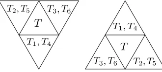
Fig. 4.1.Visualisation of the proof of Theorem 4.2.

Every edge appears twice in this sum since it is shared between two elements; hence we obtain the edge representation

δEc(y), u

=X x∈L

6 X

j=1 1

2 VTx,j,j+VTx,j−1,j

·Dju(x) ∀u∈U0. (4.6)

Since Dj+3u(x+aj) = −Dju(x), and using VT ,j+3 =−VT ,j (see (2.10)) we can reduce this sum as follows:

δEc(y), u= X

x∈L

3 X

j=1 1

2 VTx,j,j+VTx,j−1,j−VTx,j,j+3−VTx,j−1,j+3

·Dju(x)

= X x∈L

3 X

j=1

VTx,j,j+VTx,j−1,j

·Dju(x).

This concludes the proof of (4.3).

For the proof of (4.4) one only needs to use the identityDj+3u(x+aj) =−Dju(x).

Theorem 4.2. Let y∈Y0, then

δEa(y)−δEc(y)

U−1,p ≤c M2kD

3_y

k`p+M<sub>3</sub>kD2yk2<sub>`</sub>2p

(4.7)

whereM2, M3 are defined in§2.4.1.

Proof. It is useful to visualize this proof using Figure 4.1, and Figure 2.3 for additional detail. From Lemma 4.1 we obtain

δEa(y)−δEc(y), u= X

x∈L

3 X

j=1

δj(x)·Dju(x),

where δj(x) := Vx,j−Vx+aj,j+3−VTx,j,j−VTx,j−1,j. (4.8)

In the following we estimateδ1(x) only; the remaining estimates follow by symmetry. Let F+ := ∂Tx,1y and F− := ∂Tx,6y, then VTx,1,1 = VF+,1 and VTx,6,1 = VF−,1. Moreover we can Taylor expand

Vx,1= VF+,1+ 6 X

i=1

VF+,1i(Diy(x)−F+ai) +O |D

and similarly,

−Vx+a1,4= −VF−,4−

6 X

j=1

VF−,4i(Diy(x+a1)−F−ai) +O |D

2_y(x)|2

= VF−,1−

6 X

j=1

VF−,1(i+3)(Diy(x+a1)−F−ai) +O |D

2_y(x)|2

= VF−,1+

6 X

j=1

VF−,1i(−Di+3y(x+a1)−F−ai) +O |D

2_y(x)|2 .

An analysis of the remainder shows thatO(|D2_y(x)|2_)≤ 1 2

P6

i,j=1|∂1ijV(θ)| |D2y(x)|2 for someθ∈R2×6. In the remainder of the proof we will suppress the argumentθ.

Clearly, VF−,1i−VF+,1i = O(|D

2_{y(x)|) ≤} P6

j=1|∂1ijV| |D

2_{y(x)|, and hence we}

can deduce that

δ1(x) =

6 X

i=1

VF+,1i Diy(x)−F+ai−Di+3y(x+a1)−F−ai

+O |D2y(x)|2

=

6 X

i=1

VF+,1i Diy(x)−Diy(x +

i ) +Diy(x+a1−ai)−Diy(x−i )

+O |D2y(x)|2

=:

6 X

i=1

VF+,1iεi+O |D

2_y(x)|2 ,

where x+_i := xTx,1,i and x

−

i := xTx,6,i. (These are simply the vertices in the two

adjacent elements such that the identitiesF±ai=Diy(x±i ) hold.)

Carrying out the previous Taylor expansions in detail, we find that, in the last estimate,O(|D2_y(x)|2_)≤2P6

i,j=1|∂1ijV| |D2y(x)|2.

We computeε3 in detail but only give the results for the remaining coefficients:

ε3= D3y(x)−D3y(x+a1) +D3y(x+a1−a3)−D3y(x−a3)

= −D1D3y(x) +D1D3y(x−a3) =D6D1D3y(x).

By performing similar calculations fori= 1,2,4,5,6, one finds

ε1=ε2=ε6= 0, ε4=D1D1D4y(x), and ε5=D1D2D5y(x);

hence we obtain thatδj(x) =O(|D2y(x)|2+|D3y(x)|) (recall that we assumed, with-out loss of generality, thatj= 1), where O(|D3_y(x)|)≤P

i=3,4,5|∂1,iV||D 3_y(x)|.

Combining these estimates, we obtain

δEa(y)−δEc(y), u

≤ X x∈L

3 X

j=1

|δj(x)|p

1/p X

x∈L

3 X

j=1

|Dju(x)|p 01/p0

.

Finally, elementary estimates yield

X

x∈L

3 X

j=1

|δj(x)|p

1/p

≤ M2kD3yk`p+M<sub>3</sub>kD2yk2<sub>`</sub>2p, and

X

x∈L

3 X

j=1

|Dju(x)|p 01/p0

≤ 2√31/p0 X

T∈T

|T| ∂Tu

Fig. 4.2.Notation for neighbouring triangles ofT∈_T.

from which the result follows immediately.

In the following subsections, we derive technical results related to Theorem 4.2, in preparation for the proof of consistency of the GR-AC method.

4.2. Stress tensors. If there exist tensor fields Σa(y;•),Σc(y;•)∈P0(T)2×2,

for somey∈Y0, which satisfy the identities

hδEa(y), ui= X

T∈T

|T|Σa(y;T) :∂Tu, and (4.9)

hδEc(y), ui= X

T∈T

|T|Σc(y;T) :∂Tu (4.10)

then we call Σa an atomistic stress tensor and Σc a continuum stress tensor.

It follows from (4.1) and (4.2) that

Σa(y;T) :=

1 Ω0

6 X

j=1

VxT ,j,j ⊗aj, and (4.11)

Σ1_c(y;T) := ∂W(∂Ty) = 1 Ω0

6 X

j=1

VT ,j⊗aj (4.12)

satisfy, respectively, (4.9) and (4.10), however, they are not unique choices.

In the following calculation (and later on as well) we denote by Tj the unique neighbouring element ofT ∈T, which shares an edge with direction aj with T; see Figure 4.2. With this notation, and using the fact thatDju(xT ,j) =Dju(xTj,j), we

observe that

δEc(y), u= X

T∈T

|T| 1 Ω0

6 X

j=1

VT ,j·Dju(xT ,j) (4.13)

=X T∈T

|T| 1 Ω0

6 X

j=1

1

2 VT ,j+VTj,j

·Dju(xT ,j)

= X T∈T

|T|

₁

Ω0 6 X

j=1

1

2 VT ,j+VTj,j

⊗aj

:∂Tu ∀u∈U0,

which yields the alternative continuum stress tensor

Σ2_c(y;T) := 1 Ω0

6 X

j=1

1

2 VT ,j+VTj,j

Furthermore, if we write the Cauchy–Born energy in terms of the site energy (2.2), and apply the procedure used to derive Σa, then we obtain a third variant of

the continuum stress tensor:

Σ3_c(y;T) := 1 Ω0

6 X

j=1 V_xc

T ,j,j ⊗aj. (4.15)

We see that stress tensors are not uniquely defined by (4.10) and (4.9). This causes analytical difficulties when deriving modelling error estimates, which strongly depend on the choice of the stress tensors. For example we will show in the following result that Σ2_c is second-order consistent. By contrast, Σ1_c and Σ3_c are only first-order consistent (cf. Remark 4.4).

Lemma 4.3. Let y∈Y0, then

Σa(y;T)−Σ2c(y;T)

≤c M3|D2y(x)|2+M2|D3y(x)|

(4.16)

for allT ∈T, x∈T.

Proof. This estimate is obtained by reversing the construction of Σ2

c in (4.13),

and applying the estimates obtained in the proof of Theorem 4.2.

Remark 4.4. Taylor expansions show that Σkc, k = 1,3, are only first-order

consistent,

Σa(y;T)−Σkc(y;T)

≤cM2|D2y(x)| forx∈T,

but that a second-order estimate such as(4.16)would be false. The first-order estimate can also be obtained from the fact that Σa(yF;•) = Σkc(yF;•) = ∂W(F) for all F ∈

R2×2.

4.3. Divergence-free stress tensors. In the previous subsection, we have seen that the stress functions defined in (4.9) and (4.10) are not unique. It is therefore crucial to characterize all divergence-free tensors, which is the purpose of the present section. We call a piecewise constant tensor σ ∈ P0(T)2×2 divergence free, if it

satisfies

Z

R2

σ:∂udx= X T∈T

|T|σ(T) :∂Tu= 0 ∀u∈Uc. (4.17)

Divergence-free tensors can be characterised as 2D-curls of non-conforming Crouzeix– Raviart finite elements. Let N1(T) be defined by

N1(T) := n

v:_R2→_R

v|int(T)is linear for eachT ∈T vis continuous at all edge midpoints

o

. (4.18)

The degrees of freedom for functions w∈N1(T) are the nodal values at edge

mid-points,w(qf),f ∈F, and the associated nodal basis functions are denoted byζf. We have the following characterization lemma for divergence free tensor fields, which is a variant of results in [1, 14]. Although we will never use the equivalence of the characterisation explicitly, it motivates much of our subsequent analysis.

Lemma 4.5. A tensor fieldσ∈P0(T)2×2is divergence-free (i.e., satisfies(4.17))

if and only if there existsψ∈N1(T)2, such that σ=∂ψJ, whereJis the rotation by π/2.

Proof. It is easy to show that every tensor of the form σ =∂wJ, w ∈ N1(T)2

To show the reverse, let Ω be a simply connected domain, which is a union of triangles T ∈T. Suppose that the number of vertices in Ω is #V, the number of interior vertices is #VI, the number of edges in Ω is #E, and the number of triangles in Ω is #T.

We test (4.17) for all u ∈ U0 that are non-zero only in the interior of Ω. The

dimension of allσ∈P0(Ω)2×2satisfying (4.17) for thoseucan be at most 4#T−2#VI. On the other hand, the dimension of N1(Ω)2 is 2#E and the dimension of rotated

gradients of Crouzeix–Raviart functions, denoted by∂N1(Ω)2J, is 2#E−2. We will

show below that the following formula holds:

4#T−2#VI ≤2#−2, (4.19)

which immediately implies that the subspace of divergence-free tensor coincides with

∂N1(Ω)2J. Moreover, the representation is of course unique (up to a shift) and

there-fore independent of the choice of the domain.

To prove (4.19), we use the identities (the first is Euler’s formula),

#V −#E+ #T = 1, and (4.20)

3#F = 2#E−#V + #VI, (4.21)

which is obtained by a simple counting argument. (Note that #V−#VI is the number of boundary edges.) Subtracting (4.20) from (4.21) yields (4.19).

4.4. Continuum stress tensor correctors. We have different forms of con-tinuum stress Σ1

c, Σ2c and Σ3c, which all can be used to represent δEc in the form

(4.10), and hence their differences must be divergence free. Lemma 4.5 characterises the form of these differences and motivates the following result.

Lemma 4.6. Let y ∈Y0, then there exists a corrector ψ23(y;•)∈N1(T)2

satis-fying the following two properties:

Corrector property: Σ3_c(y;T)−Σ2_c(y;T) = ∂ψ23(y;T)J ∀T ∈T; (4.22)

Lipschitz property: ψ23(y;mf)

≤ 1₆M2kD2yk`∞_(f∩L) ∀f ∈F. (4.23)

Proof. Property (4.22) follows of course from Lemma 4.5, however, to

estab-lish (4.23) we require an explicit expression ofψ23. We give the details of the proof for the case of an upward pointing triangleT ∈T (cf. the left configuration in Fig-ure 4.2). An elementary computation, starting from (4.14) and (4.15) and using the symmetry property (2.10), yields

Σ3_c(y;T)−Σ2_c(y;T) = 1 3Ω0

(VT ,1−VT1,1) + (VT ,3−VT1,3) + (VT ,5−VT1,5)

⊗a1

+. . . ,

where “. . .” stands for terms that are symmetric to the ones in the first line. The directionsa1, a3, a5are chosen anti-clockwise with respect to the elementT.

We now observe that, iff is an edge ofT with directionaj, j∈ {1,3,5}, then

∂ζfJ=

(

−2 Ω0a

>

j, in T,

2 Ω0a

>

j, in Tj.

Letf be the edge ofT with directiona1, then choosing

ψ23(y;mf) := 1

6(VT ,1−VT1,1) +

1

6(VT ,3−VT1,3) +

1

6(VT ,5−VT1,5), (4.25)

and making analogous choices for the remaining edges, we obtain (4.22).

With this explicit representation we can now prove the Lipschitz property (4.23). Letf denote the edge ofT with direction a1, F:=∂Ty andF1:=∂T1y; then

ψ23(y;mf)

≤ 1₆

VF1,1−VF,1 +1₆

VF1,2−VF,2 +1₆

VF1,3−VF,3

(4.26)

≤ 1 6

6 X

j=1

|V,1j|+|V,2j|+|V,3j|

(F1−F)aj

≤1₆M2 max

j=1,...,6

(F1−F)aj

,

whereV,1j =∂1jV(Gj·a) for someGj ∈R2×2, and M2 is defined in§2.4.1. One now

verifies that

(F1−F)a1= 0, (F1−F)a2=D6D2y(xT ,1), and (F1−F)a3=D5D3y(xT ,5),

which implies

max j=1,...,6

(F1−F)aj

≤max |D2y(xT ,1)|,|D2y(xT ,4)|.

Combining this estimate with (4.26) we obtain (4.23) for edges aligned witha1. The remaining cases follow from symmetry considerations.

5. Consistency of the GR-AC Method. We are now ready to state the

second main result of this paper. The proof is established in §5.1 through §5.3. For the remainder of this section we assume that the hypotheses stated in Theorem 5.1 hold.

Theorem 5.1. Let Eac be defined by (3.4), with parameters(Cx,i,j)6i,j=1,x∈ I,

satisfying the one-sidedness condition (3.1), as well as the patch test conditions (3.3)

and (3.9). Suppose in addition that the parameters are bounded, that is,

sup x∈I

max

j,i∈{1,...,6}|Cx,j,i|=: ¯C <+∞.

Then there exists a constant CI =CI( ¯C), such that

δEac(y)−δEa(y)

U−1,p≤c CIM2kD

2_yk

`p<sub>(I</sub>ext<sub>)</sub>+M2kD3yk<sub>`</sub>p_(C)+M3kD2yk2_`2p_(C)

,

(5.1)

whereIext _{:={x∈ L}

dist(x,I)≤1}is an extended interface region.

5.1. An a/c stress tensor. Following the construction of Σain (4.11) (withEa

replaced byEac), we obtain a representation ofδEac in terms of an a/c stress Σac: let y∈Y0andu∈U0, then

δEac(y), u

= X T∈T

|T|Σac(y;T) :∂Tu, where (5.2)

Σac(y;T) :=

1 Ω0

6 X

j=1

and we recall thatVac

x,j =∂jVac(x;Dy(x)). We now require the following additional notation:

TA:= {T ∈T |T∩(I ∪ C) =∅}, FA:= F ∩TA,

TC := {T ∈T |T∩(I ∪ A) =∅}, FC := F ∩TC, (5.4) TI:= T \(TC∪TA), and FI:= F \(FC∪FA).

Lemma 5.2. (i) LetΣac be defined by (5.3), then, for ally∈Y0,

Σac(y;T) = Σa(y;T) ∀T ∈TA, and (5.5)

Σac(y;T) = Σ3c(y;T) ∀T ∈TC. (5.6)

(ii) LetF∈R2×2; then there exists a unique ψac(F;•)∈N1(T)2 such that

Σac(yF;T)−Σa(yF;T) = ∂ψac(F;T)J ∀T ∈T, and (5.7)

ψac(F;mf) = 0 ∀f ∈FA∪FC. (5.8)

Moreover, there exists Lac depending only on C¯ such that the following Lipschitz

property holds:

ψac(F;mf)−ψac(G;mf)

≤LacM2|F−G| ∀F,G∈R2×2, f ∈FI. (5.9)

Proof. (i) Properties (5.5) and (5.6) follow immediately from the definitions of the three tensors and the sets TA andTC, and are independent of the choice of the reconstruction parameters at the interface.

(ii) SinceEac is assumed to satisfy local force consistency (3.9), we have

0 =

δEac(yF)−δEa(yF), u= X

T∈T

|T|(Σac(yF;T)−Σa(yF;T)) :∂Tu ∀u∈U0,

and hence Σac(yF;•)−Σa(yF;•) is divergence free. According to Lemma 4.5 there

exists a function ψac _{∈ N}

1(T)2, which is unique up to a constant shift, such that

(5.7) holds. Property (5.8) uniquely determines the shift.

As a matter of fact, it is highly non-trivial whether (5.8) can be satisfied, and it is in principle possible that the corrections “propagate” into the continuum region [10]. We postpone the detailed computations required to prove this to Appendix 6.1 and 6.2, where we then also give a proof of the Lipschitz property (5.9).

5.2. The modified a/c stress. The functionψac_{(F;•) obtained in Lemma 5.2}

provides the divergence-free corrector for Σac −Σa for homogeneous deformations.

We now construct a corrector for nonlinear deformations. We will defineΣbac(y;T) :=

Σac(y;T)−∂ψˆac(y;T)J, where we choose ˆψacin such a way thatΣbac(yF;T) = Σa(yF;T),

which can be achieved by ensuring that ˆψac_(y

F;mf) = ψac(F;mf) for all edge mid-pointsmf. In addition, we will impose other convenient properties ofΣbac, summarized

in Lemma 5.3 below.

First, for eachf ∈FI,f =T+∩T−, we set

Ff(y) :=1₂ ∂T+y+∂T−y

.

We can now define the corrector function fory∈Y0as

ˆ

ψac(y;•) := X f∈FI

ψac Ff(y);mfζf+

X

f∈FC

wheremf is the midpoint of edgef, and the corresponding modified stress function

b

Σac(y;T) := Σac(y;T)−∂ψˆac(y;T)J, forT∈T. (5.11)

where ζf is the nodal basis of the non-conforming Crouzeix–Raviart finite elements N1(T) (4.18). By Lemma 4.5,∂ζfJand∂ψˆac(y;T)Jare divergence free.

We show in Remark 6.1, that ˆψac is non-trivial, that is, there exists no choice of parameters for which ˆψac= 0, even under purely homogeneous deformations.

Lemma 5.3. LetΣbacbe defined by(5.11), andy∈Y0; then the following identities

hold:

hδEac(y), ui= X

T∈T

|T|Σbac(y;T) :∂Tu ∀u∈U0; (5.12)

b

Σac(y;T) = Σa(y;T) ∀T ∈TA; (5.13)

b

Σac(y;T) = Σ2c(y;T) ∀T ∈TC; and (5.14)

b

Σac(yF;•) = Σa(yF;•) ∀F∈R2×2. (5.15)

Moreover, there exists a constantLacˆ , which depends only on C¯, such that

bΣac(y;T)−Σbac(yF;T)

≤LacM2ˆ kD2yk`∞_(T∩L) ∀T ∈T_I, F=∂_Ty. (5.16)

Proof. Identity (5.12) follows from (5.2) and the fact thatΣbac−Σacis

divergence-free.

Identity (5.13) follows from (5.5) and the fact that ˆψac(y;mf) = 0 for allf ∈FA, which implies thatΣbac(y;T) = Σac(y;T) = Σa(y;T) for allT ∈TA. Similarly, (5.14) follows from (5.6), and the fact that ˆψac=ψ23 in all elementsT ∈TC.

FixF∈R2×2. To prove (5.15) we first note that, since ψ23(yF;•) = 0, we have

ˆ

ψac_(y

F;•) =ψac(F;•). Using (5.7), we obtain

b

Σac(yF;•) = Σac(F;•)−∂ψac(F;•)J= Σa(yF;•).

We are only left to prove the Lipschitz property (5.16). WithF:=∂Ty, we have

bΣac(y;T)−Σbac(yF;T) ≤

Σac(y;T)−Σac(yF;T) +

∂ψˆac(y;T)−∂ψˆac(yF;T) . (5.17)

From its definition (5.3), and the fact that second partial derivatives ofV are globally bounded, it is clear that Σac satisfies a Lipschitz property of the form

Σac(y;T)−Σac(yF;T)

≤L1M2kD2yk`∞_(T∩L) (5.18)

where L1 depends only on ¯C; see also [10, Lemma 19] for a similar result. (If the

reconstruction parameters satisfy the one-sidedness condition (3.1), as well as the patch test conditions (2.6), (2.7), one may show thatL1= 3 ¯C/Ω0.)

To bound the second term on the right-hand side in (5.17) we invoke the inverse inequality

∂ψˆac(y;T)−∂ψˆac(yF;T) ≤

2 Ω0

X

f∈F

f⊂T

ψˆac(y;mf)−ψˆac(yF;mf)

where we used the fact that|∂ζf|= 2/Ω0for allf ∈F. Iff ∈FA, then ˆψac(•;mf) = 0. Iff ∈FC, then ˆψac(•;mf) =ψ23(•;mf) and hence, using (4.23),

ψˆac(y;mf)−ψˆac(yF;mf)

=

ψ23(y;mf)

≤ 1₆M2kD2yk`∞_(T∩L).

If f ∈ FI, then ˆψac(y;mf) = ψac(Ff;mf) and ˆψac(yF;mf) = ψac(F;mf). We can therefore employ (5.9) to estimate

ψˆac(y;mf)−ψˆac(yF;mf)

=

ψac(Ff;mf)−ψac(F;mf)

≤ LacM2 Ff−F

≤ Lac_2ΩM2 0 kD

2_y

k`1_(T∩L).

The last inequality can be verified through straightforward geometric arguments. Without explicit constants its validity is obvious.

Combining the two foregoing estimates, we obtain

∂ψˆac(y;T)−∂ψˆac(yF;T)

≤cmax(Lac,1)M2kD2yk`∞_(L∩T). (5.19)

Combining (5.17), (5.18) and (5.19), yields (5.16).

5.3. Proof of Theorem 5.1. With the preparations of the foregoing sections it is now easy to complete the proof of the main consistency result, Theorem 5.1. Again, we drop the dependence ony whenever possible. We begin by splitting the modelling error into a continuum contribution and an interface contribution,

hδEac−δEa, ui = X

T∈T

|T| b

Σac(T)−Σa(T)

:∂Tu

= X T∈TC

|T| b

Σac(T)−Σa(T)

:∂Tu+

X

T∈TI |T|

b

Σac(T)−Σa(T)

:∂Tu

=: EC+ EI,

and estimate EC and EI separately. Note also that we used (5.13) to drop the sum over elements in the atomistic region.

Using the fact that Σbac = Σ2c in TC, (5.14), and the stress estimate (4.16), we

obtain

EC ≤ X T∈TC

|T| Σ

2

c(T)−Σa(T) |∂Tu|

≤ c X

x∈C

M2|D3y(x)|+M3|D2y(x)|2p1/p X

T∈TC

|T||∂Tu|p 01/p0

≤ cM2kD3yk`p<sub>(C)</sub>+M3kD2yk2<sub>`</sub>2p_(C)

X

T∈T

|T||∂Tu|p 01/p0

. (5.20)

To estimate EI, we employ the Lipschitz property (5.16) for Σbac and the fact

that Σac = Σa under homogeneous deformations (see (5.15)). Using (2.8) it is also

straightforward to prove

Σa(y;T)−Σa(yF;T) ≤ _Ω1

0M2kD 2_yk

`∞_(T∩L) ∀T ∈T, F=∂Ty. (5.21)

Using (5.15), (5.16) and (5.21),we obtain, for anyT ∈TI,

bΣac(y;T)−Σa(y;T) ≤

bΣac(y;T)−Σbac(yF;T) +

Σa(y;T)−Σa(yF;T)

≤ LˆacM2kD2yk`∞_(T∩L)+_Ω1

0M2kD 2_yk

and summing overT ∈TI yields

EI≤ X T∈TI

|T|( ˆLac+_Ω1

0)M2kD 2_yk

`∞_(T∩L)|∂_Tu|

≤ cCIM2kD2yk`p_(Iext₎ X

T∈T

|T| |∂Tu|p 01/p0

, (5.22)

whereCI depends only on ˆLac, which depends only on ¯C.

Combining (5.22) and (5.20) we finally obtain the desired modelling error estimate (5.1). This concludes the proof of Theorem 5.1.

6. Appendix: Proof of Lemma 5.2 (ii). In this appendix, we provide the remaining details for the proof of Lemma 5.2(ii). Throughout this proof we fix a homogeneous deformation yF, F ∈ R2×2, and drop the argument y = yF whenever

possible. For example, we will write Σac(T) = Σac(yF;T).

We begin by computing an expression for Σac−Σa in terms of the parameters Cx,j. Equation (3.8), in the proof of Lemma 3.2, can be rewritten in the form

V_x,ac_F,j :=∂jVxac(Fa) = (1−Cx,j−1)VF,j−1+Cx,jVF,j+ (1−Cx,j+1)VF,j+1.

Recalling also (4.11) and usingaj =aj−1+aj+1, we obtain

Σac(T)−Σa(T) = 6 X

j=1

VxacT ,j,F,j−VF,j

⊗aj

= 1 Ω0

6 X

j=1

(1−CxT ,j,j−1)VF,j−1+ (CxT ,j,j −1)VF,j+ (1−CxT ,j,j+1)VF,j+1

⊗aj

= 1 Ω0

6 X

j=1 VF,j⊗

(1−CxT ,j−1,j)aj−1+ (CxT ,j,j−1)aj+ (1−CxT ,j+1,j)aj+1

= 1 Ω0

6 X

j=1 VF,j⊗

−CxT ,j−1,jaj−1+CxT ,j,jaj−CxT ,j+1,jaj+1

. (6.1)

The explicit evaluation of (6.1) for interface elements is carried out separately for flat interfaces and interfaces with corners.

For triangles not intersecting the interface, Σac(yF;T)−Σa(yF;T) = 0, hence we

need to compute the stress errors only for interface elements.

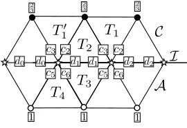
6.1. Flat interface. Consider the flat interface configuration in Figure 6.1. Ac-cording to (3.10) and (3.11) the free parameters are cj := Cx,j (for x ∈ I and

j ∈ {2,3,5,6}), and di, i ∈ Z, where d1 = CxT2,1,1 = CxT2,4,4, and so forth. We

calculate the a/c stress for the elementsT1, T2, and collect the results in Table 6.1.

From Table 6.1 we can read off the stress differences Σac−Σa in the elements T1, T2:

Σac(T1)−Σa(T1) =(2₃−d2)VF,1+ (c2−2₃)VF,2+ (2₃−c3)VF,3 ⊗_Ωa2 0

+

Fig. 6.1.Visualisation of the flat interface analysis in§6.1.

Table 6.1

Table of coefficients ofVF,j in (6.1), in interfacial triangles, on flat interfaces.

j Cx_{T ,j}−1,j CxT ,j,j CxT ,j+1,j −CxT ,j−1,jaj−1+CxT ,j,jaj−CxT ,j,j+1aj+1

T1

1 2₃ 2₃ d2 −2₃a6+2₃a1−d2a2= (2₃−d2)a2

2 2

3 c2 c2 −

2

3a1+c2a2−c2a3= (− 2

3+c2)(a2−a3) 3 c3 c3 2₃ −c3a2+c3a3−2₃a4= (2₃−c3)(a2−a3) 4 d1 2₃ 2₃ −d1a3+2₃a4−2₃a5= (2₃−d1)a3

5 2₃ 2₃ 2₃ 0

6 2₃ 2₃ 2₃ 0

T2

1 2₃ d1 d1 −2₃a6+d1a1−d1a2= (2₃−d1)a3

2 c2 c2 c2 0

3 c3 c3 c3 0

4 d1 d1 2₃ −d1a3+d1a4−2₃a5= (2₃−d1)a2 5 c5 2₃ 2₃ −c5a4+2₃a5−2₃a6= (c5−2₃)a1

6 2

3

2

3 c6 −

2 3a5+

2

3a6−c6a1= ( 2 3−c6)a1

and

Σac(T2)−Σa(T2) =(d1−2₃)VF,1+ (2₃−c5)VF,2+ (c6−2₃)VF,3 ⊗_Ωa1 0

=

(d1−2₃)VF,1+ (2₃−c2)VF,2+ (c3−2₃)VF,3 ⊗_Ωa2₀

−

(d1−2

3)VF,1+ ( 2

3−c2)VF,2+ (c3− 2

3)VF,3 ⊗

a3 Ω0

+

(c2−c5)VF,2+ (c6−c3)VF,3 ⊗_Ωa1 0.

Note that we have provided two alternative representations of Σac(T2)−Σa(T2), since

the first representation is in general insufficient to construct the corrector.

Since the atomistic region is a mirror image of the continuum region with respect to the interface, we can obtain stress function Σac(yF;·) forT3andT4from symmetry

considerations:

Σac(T4)−Σa(T4) =

(1−d0)VF,1+ (c5−1)VF,2+ (1−c6)VF,3 ⊗_Ωa2₀

+(d1−1)VF,1+ (1−c5)VF,2+ (c6−1)VF,3 ⊗_Ωa3 0,

and

Σac(T3)−Σa(T3) =

(d1−1)VF,1+ (1−c2)VF,2+ (c3−1)VF,3 ⊗Ωa10

=(d1−1)VF,1+ (1−c5)VF,2+ (c6−1)VF,3 ⊗_Ωa2₀

−

(d1−1)VF,1+ (1−c5)VF,2+ (c6−1)VF,3 ⊗_Ωa3 0

−

Fig. 6.2.Interface configuration with corner.

From the proof Lemma 4.6 recall that∂ζf(T)J=−_Ω2

0aj iff is an edge ofT and ajthe counter-clockwise direction of the edge (relative toT). We can therefore choose

ψac explicitly, for example, forf =T1∩T2:

ψac(F;mf) := 1₂(d1−2₃)VF,1+ (2₃−c2)VF,2+ (c3−2₃)VF,3 . (6.2)

For the remaining edges, similar choices can be made, the crucial observation being that the terms in neighbouring elements associated with an edge cancel each other out.

We observe, moreover, that for the trianglesT1andT4, thea1components of the

stresses vanish, which means that ψac_(F;m

f) = 0 for allf ∈FA∪FC. This proves (5.8) in the flat interface case.

It remains to prove the Lipschitz bound (5.9). From (6.2) (and the corresponding formulas for the remaining edges), it is straightforward to show thatψac _{is Lipschitz}

continous for any fixed set of parameters with a Lipschitz constant of the formLM2, where Lcan be bounded in terms of ¯C. This concludes the proof of Lemma 5.2 (ii) in the flat interface case.

Remark 6.1 (Correctors are neccessary). From the calculation in this section,

it is clear that one cannot choose parameters such thatΣac(yF;T) = Σa(yF;T)for all T ∈T and for all potentials V ∈V. For example, ifΣac(yF;T2) = Σa(yF;T2) for all V, thend1= 2/3, whereas ifΣac(yF;T3) = Σa(yF;T3), thend1= 1. This demonstrates

that the divergence-free corrector fields are in fact necessary, and that it is impossible in our current framework to construct an a/c method where Σac(yF;T) = Σa(yF;T)

holds for allT ∈T,F∈R2×2, andV ∈V.

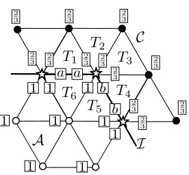
6.2. General interface. We now turn to the proof of (5.7)– (5.9) for interface configurations with corners. Consider the corner configuration displayed in Figure 6.2, which is concave from the point of view of the atomistic region. The reconstruction coefficients found in Proposition 3.7 are displayed in the figure as well. Recall that the reconstructions of bonds into the atomistic or continuum regions are now uniquely determined, while the bonds lying at the interfaces (parametersaandb) are still free.

Fig. 6.3.All possible corner configurations (up to translation, rotation and reflection).

T1, . . . , T6 can again be computed explicitly:

Σac(T1)−Σa(T1) = (1₃VF,3−1₃VF,2)⊗a01+ (a− 2

3)VF,1⊗a

0

2−(a− 2

3)VF,1⊗a

0

3,

Σac(T2)−Σa(T2) = (a−2₃)VF,1⊗a03,

Σac(T3)−Σa(T3) = (b−2₃)VF,3⊗a01,

Σac(T4)−Σa(T4) = −(b−2₃)VF,3⊗a01+ (b− 2

3)VF,3⊗a

0

2+ ( 1 3VF,1−

1

3VF,2)⊗a

0

3,

Σac(T5)−Σa(T5) = (1₃VF,2−1₃VF,1)⊗a03+ [(1−a)VF,1+ (b−1)VF,3]⊗a02

−(b−1)VF,3⊗a01, and

Σac(T6)−Σa(T6) = (1₃VF,2−1₃VF,3)⊗a01+

(a−1)VF,1+ (1−b)VF,3

⊗a0₂

−(a−1)VF,1⊗a03.

Following the argument in §6.1, we can check again that the associated edge contri-butions from neighbouring elements cancel, and hence we can explicitly construct the corrector function ψac_{. Note that Σ}

ac(T2) has noa01 component and Σac(T5) has no a0₃ component, which implies (5.8).

For a corner that is convex from the point of view of the atomistic region, the result follows by symmetry (interchanging the coefficients 1 and 2₃). The Lipschitz bound (5.9) can be obtained from the above formulas, under the assumption that the reconstruction coefficientsa, bare bounded above by ¯C.

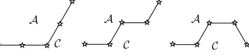
Finally, we have to convince ourselves that our above argument applies to all possible interface geometries. In Figure 6.3 we present an exhaustive list, up to trans-lations, rotations and reflections, of local interface geometries. (Recall our geometric requirements formulated in Assumption 3.6.) By inspecting the calculation of the stress differences Σac−Σa for the case presented in Figure 6.2, one observes that

the formulas are local, and do not depend on the extended geometry of the interface. We note, however, that this only holds due to the separation Assumption 3.6. The subsequent construction of the corrector now follow of course verbatim.

This concludes the proof of Lemma 5.2(ii)in the general interface case.

7. Conclusion. We have shown for a 2D model problem that it is possible to construct patch test consistent a/c coupling method for many-body potentials, in interface geometries with corners, using a new variant of the geometry reconstruction technique introduced in [4, 18], which we labelled the GR-AC method. Moreover, we have proven a quasi-optimal modelling error estimate for the GR-AC method(s) we constructed.

We see this work as a first step towards a general theory of GR-AC method(s). Our goal is to show eventually that the free parameters in the method can always

(that is, in any dimension, for any interface geometry) be determined so as to satisfy the energy and force consistency conditions, and that the resulting GR-AC method(s) will have the same consistency properties that we establish in the present case.

pa-rameters does the GR-AC method have sharp stability properties as discussed in [3]? This issue is the topic of ongoing research.

REFERENCES

[1] Douglas N. Arnold and Richard S. Falk. A uniformly accurate finite element method for the Reissner-Mindlin plate.SIAM J. Numer. Anal., 26(6):1276–1290, 1989.

[2] M. Dobson and M. Luskin. An optimal order error analysis of the one-dimensional quasicon-tinuum approximation.SIAM Journal on Numerical Analysis, 47(4):2455–2475, 2009. [3] M. Dobson, M. Luskin, and C. Ortner. Accuracy of quasicontinuum approximations near

instabilities.J. Mech. Phys. Solids., 58(10):1741–1757, 2010.

[4] W. E, J. Lu, and J.Z. Yang. Uniform accuracy of the quasicontinuum method.Phys. Rev. B, 74(21):214115, 2006.

[5] W. E and P. Ming. Cauchy-Born rule and the stability of crystalline solids: static problems.

Arch. Ration. Mech. Anal., 183(2):241–297, 2007.

[6] J. Lu and P. Ming. Convergence of a force-based hybrid method for atomistic and continuum models in three dimensions. arXiv:1102.2523v2.

[7] R. Miller and E. Tadmor. A unified framework and performance benchmark of fourteen mul-tiscale atomistic/continuum coupling methods. Modelling Simul. Mater. Sci. Eng., 17, 2009.

[8] P. Ming and J. Z. Yang. Analysis of a one-dimensional nonlocal quasi-continuum method.

Multiscale Modeling & Simulation, 7(4):1838–1875, 2009.

[9] M. Ortiz, R. Phillips, and E. B. Tadmor. Quasicontinuum analysis of defects in solids. Philo-sophical Magazine A, 73(6):1529–1563, 1996.

[10] C. Ortner. The role of the patch test in 2d atomistic-to-continuum coupling methods. arXiv:1101.5256.

[11] C. Ortner. A priori and a posteriori analysis of the quasi-nonlocal quasicontinuum method in 1d.Math. Comp., 80:1265–1285, 2011.

[12] C. Ortner and A. V. Shapeev. Analysis of an energy-based atomistic/continuum coupling approximation of a vacancy in the 2d triangular lattice. arXiv:1104.0311.

[13] C. Ortner and H. Wang. Coarse graining in energy-based quasicontinuum methods. To appear in Math. Models Meth. Appl. Sc.

[14] K. Polthier and E. Preuss. identifying vector field singularities using a discrete hodge decom-position. InVisualization and Mathematics III. Springer Verlag, 2002.

[15] A. Shapeev. Consistent energy-based atomistic/continuum coupling for two-body potentials in three dimensions. arXiv:1108.2991.

[16] A. V. Shapeev. Consistent energy-based atomistic/continuum coupling for two-body potentials in one and two dimensions.Multiscale Model. Simul., 9:905–932, 2011.

[17] V. B. Shenoy, R. Miller, E. B. Tadmor, D. Rodney, R. Phillips, and M. Ortiz. An adaptive finite element approach to atomic-scale mechanics–the quasicontinuum method. J. Mech. Phys. Solids, 47(3):611–642, 1999.