Proceedings of the 2011 Conference on Empirical Methods in Natural Language Processing, pages 284–293,
Linear Text Segmentation Using Affinity Propagation
Anna Kazantseva School of Electrical Engineering
and Computer Science, University of Ottawa
Stan Szpakowicz
School of Electrical Engineering and Computer Science, University of Ottawa & Institute of Computer Science,
Polish Academy of Sciences
Abstract
This paper presents a new algorithm for lin-ear text segmentation. It is an adaptation of Affinity Propagation, a state-of-the-art clus-tering algorithm in the framework of factor graphs. Affinity Propagation for Segmenta-tion, orAPS, receives a set of pairwise simi-larities between data points and produces seg-ment boundaries and segseg-mentcentres – data points which best describe all other data points within the segment. APS iteratively passes messages in a cyclic factor graph, until conver-gence. Each iteration works with information on all available similarities, resulting in high-quality results.APSscales linearly for realistic segmentation tasks. We derive the algorithm from the original Affinity Propagation formu-lation, and evaluate its performance on topi-cal text segmentation in comparison with two state-of-the art segmenters. The results sug-gest thatAPSperforms on par with or outper-forms these two very competitive baselines.
1 Introduction
In complex narratives, it is typical for the topic to shift continually. Some shifts are gradual, others – more abrupt.Topical text segmentationidentifies the more noticeable topic shifts. A topical segmenter’s output is a very simple picture of the document’s structure. Segmentation is a useful intermediate step in such applications as subjectivity analysis (Stoy-anov and Cardie, 2008), automatic summarization (Haghighi and Vanderwende, 2009), question an-swering (Oh, Myaeng, and Jang, 2007) and others. That is why improved quality of text segmentation can benefit other language-processing tasks.
We present Affinity Propagation for Segmenta-tion (APS), an adaptation of a state-of-the-art clus-tering algorithm, Affinity Propagation (Frey and Dueck, 2007; Givoni and Frey, 2009).1 The
origi-nal AP algorithm considerably improved exemplar-based clustering both in terms of speed and the qual-ity of solutions. That is why we chose to adapt it to segmentation. At its core, APSis suitable for seg-menting any sequences of data, but we present it in the context of segmenting documents. APStakes as input a matrix of pairwise similarities between sen-tences and, for each sentence, a preference value which indicates an a priori belief in how likely a sentence is to be chosen as a segment centre.
APSoutputs segment assignments and segment cen-tres – data points which best explain all other points in a segment. The algorithm attempts to maximize
net similarity – the sum of similarities between all data points and their respective segment centres.
APS operates by iteratively passing messages in a factor graph (Kschischang, Frey, and Loeliger, 2001) until a good set of segments emerges. Each iteration considers all similarities – takes into ac-count all available information. An iteration in-cludes sending at most O(N2) messages. For the
majority of realistic segmentation tasks, however, the upper bound is O(M N) messages, where M
is a constant. This is more computationally ex-pensive than the requirements of locally informed segmentation algorithms such as those based on HMM or CRF (see Section 2), but for a globally-informed algorithm the requirements are very rea-sonable.APSis an instance of loopy-belief propaga-tion (belief propagapropaga-tion on cyclic graphs) which has
1An implementation ofAPSin Java, and the data sets, can be
downloaded athwww.site.uottawa.ca/∼ankazanti.
been used to achieved state-of-the-art performance in error-correcting decoding, image processing and data compression. Theoretically, such algorithms are not guaranteed to converge or to maximize the objective function. Yet in practice they often achieve competitive results.
APSworks on an already pre-compiled similaritiy matrix, so it offers flexibility in the choice of simi-larity metrics. The desired number of segments can be set by adjusting preferences.
We evaluate the performance of APS on three tasks: finding topical boundaries in transcripts of course lectures (Malioutov and Barzilay, 2006), identifying sections in medical textbooks (Eisen-stein and Barzilay, 2008) and identifying chapter breaks in novels. We compareAPSwith two recent systems: the Minimum Cut segmenter (Malioutov and Barzilay, 2006) and the Bayesian segmenter (Eisenstein and Barzilay, 2008). The comparison is based on the WindowDiff metric (Pevzner and Hearst, 2002). APS matches or outperforms these very competitive baselines.
Section 2 of the paper outlines relevant research on topical text segmentation. Section 3 briefly cov-ers the framework of factor graphs and outlines the original Affinity Propagation algorithm for cluster-ing. Section 4 contains the derivation of the new update messages for APSeg. Section 5 describes the experimental setting, Section 6 reports the results, Section 7 discusses conclusions and future work.
2 Related Work
This sections discusses selected text segmentation methods and positions the proposedAPS algorithm in that context.
Most research on automatic text segmentation re-volves around a simple idea: when the topic shifts, so does the vocabulary (Youmans, 1991). We can roughly subdivide existing approaches into two cat-egories: locally informed and globally informed.
Locally informed segmenters attempt to identify topic shifts by considering only a small portion of complete document. A classical approach is Text-Tiling (Hearst, 1997). It consists of sliding two ad-jacent windows through text and measuring lexical similarity between them. Drops in similarity corre-spond to topic shifts. Other examples include text
segmentation using Hidden Markov Models (Blei and Moreno, 2001) or Conditional Random Fields (Lafferty, McCallum, and Pereira, 2001). Locally informed methods are often very efficient because of lean memory and CPU time requirements. Due to a limited view of the document, however, they can easily be thrown off by short inconsequential digres-sions in narration.
Globally informed methods consider “the big pic-ture” when determining the most likely location of segment boundaries. Choi (2000) applies divisive clustering to segmentation. Malioutov and Barzilay (2006) show that the knowledge about long-range similarities between sentences improves segmenta-tion quality. They cast segmentasegmenta-tion as a graph-cutting problem. The document is represented as a graph: nodes are sentences and edges are weighted using a measure of lexical similarity. The graph is cut in a way which maximizes the net edge weight within each segment and minimizes the net weight of severed edges. SuchMinimum Cutsegmentation resemblesAPSthe most among others mentioned in this paper. The main difference between the two is in different objective functions.
Another notable direction in text segmentation uses generative models to find segment boundaries. Eisenstein and Barzilay (2008) treat words in a sen-tence as draws from a multinomial language model. Segment boundaries are assigned so as to maximize the likelihood of observing the complete sequence. Misra et al. (2009) use a Latent Dirichlet alloca-tion topic model (Blei, Ng, and Jordan, 2003) to find coherent segment boundaries. Such methods output segment boundaries and suggest lexical distribution associated with each segment. Generative models tend to perform well, but are less flexible than the similarity-based models when it comes to incorpo-rating new kinds of information.
Globally informed models generally perform bet-ter, especially on more challenging datasets such as speech recordings, but they have – unsurprisingly – higher memory and CPU time requirements.
docu-ment (or all of it). BecauseAPSoperates on a pre-compiled matrix of pair-wise sentence similarities, it is easy to incorporate new kinds of information, such as synonymy or adjacency. It also provides some in-formation as to what the segment is about, because each segment is associated with a segment centre. 3 Factor graphs and affinity propagation
for clustering
3.1 Factor graphs and the max-sum algorithm
The APS algorithm is an instance of belief propa-gation on a cyclic factor graph. In order to explain the derivation of the algorithm, we will first briefly introduce factor graphs as a framework.
Many computational problems can be reduced to maximizing the value of a multi-variate function
F(x1, . . . , xn)which can be approximated by a sum
of simpler functions. In Equation 1, H is a set of
discrete indices andfhis a local function with
argu-mentsXh⊂ {x1, . . . , xn}:
F(x1, . . . , xn) = X
h∈H
fh(Xh) (1)
Factor graphs offer a concise graphical represen-tation for such problems. A global functionFwhich
can be decomposed into a sum ofM local function fh can be represented as a bi-partite graph with M
function nodes andN variable nodes (M = |H|). Figure 1 shows an example of a factor graph for
F(x1, x2, x3, x4) =f1(x1, x2, x3) +f2(x2, x3, x4). The factor (or function) nodes are dark squares, the variable nodes are light circles.
The well-known max-sum algorithm (Bishop, 2006) seeks a configuration of variables which max-imizes the objective function. It finds the maximum in acyclic factor graphs, but in graphs with cycles neither convergence nor optimality are guaranteed (Pearl, 1982). Yet in practice good approximations can be achieved. The max-sum algorithm amounts to propagating messages from function nodes to variable nodes and from variable nodes to function nodes. A message sent from a variable nodexto a function nodef is computed as a sum of the
incom-ing messages from all neighbours ofxother thanf
(the sum is computed for each possible value ofx):
µx→f = X
f0∈N(x)\f
µf0→x (2)
Figure 1: Factor graph forF(x1, x2, x3, x4)
=f1(x1, x2, x3) +f2(x2, x3, x4).
f1 f2
x1 x2 x3 x4
N(x) is the set of all function nodes which arex’s
neighbours. The message reflects the evidence about the distribution ofxfrom all functions which havex
as an argument, except for the function correspond-ing to the receivcorrespond-ing nodef.
A messageµf→xfrom functionf to variablexis
computed as follows:
µf→x= max
N(f)\x(f(x1, . . . , xm) + X
x0∈N(f)\x
µx0→f)
(3)
N(f)is the set of all variable nodes which aref’s
neighbours. The message reflects the evidence about the distribution ofxfrom functionf and its neigh-bours other thanx.
A common message-passing schedule on cyclic factor graphs is flooding: iteratively passing all variable-to-function messages, then all function-to-variable messages. Upon convergence, the summary message reflecting final beliefs about the maximiz-ing configuration of variables is computed as a sum of all incoming function-to-variable messages.
3.2 Affinity Propagation
TheAPSalgorithm described in this paper is a mod-ification of the original Affinity Propagation algo-rithm intended for exemplar-based clustering (Frey and Dueck, 2007; Givoni and Frey, 2009). This sec-tion describes the binary variable formulasec-tion pro-posed by Givoni and Frey, and lays the groundwork for deriving the new update messages (Section 4).
Affinity Propagation for exemplar-based cluster-ing is formulated as follows: to cluster N data
points, one must specify a matrix of pairwise sim-ilarities {SIM(i, j)}i,j∈{1,...,N},i6=j and a set of
self-similarities (so-called preferences) SIM(j, j)
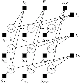
Figure 2: Factor graph for affinity propagation.
E1 Ej EN
I1
Ii
IN
c11 c1j c1N
ci1 cij ciN
cN1 cN j cN N
S11 S1j S1N
Si1 Sij SiN
SN1 SN j SN N
similarities between all points and their respective exemplars; this is expressed by Equation 7. Figure 2 shows a schematic factor graph for this problem, withN2 binary variables. c
ij = 1 iff pointj is an
exemplar for pointi. Function nodesEj enforce a
coherence constraint: a data point cannot exemplify another point unless it is an exemplar for itself:
Ej(c1j, . . . , cN j) =
−∞ ifcjj = 0 ∧ cij = 1
for somei6=j 0 otherwise
(4)
AnI node encodes asingle-cluster constraint: each
data point must belong to exactly one exemplar – and therefore to one cluster:
Ii(ci1, . . . , ciN) = (
−∞ if Pjcij 6= 1
0 otherwise (5)
An S node encodes user-defined similarities between data-points and candidate exemplars (SIM(i, j) is the similarity between points i and j):
Sij(cij) = (
SIM(i, j) ifcij = 1
0 otherwise (6)
Equation 7 shows the objective function which we want to maximize: a sum of similarities between data points and their exemplars, subject to the two
constraints (coherence and single-cluster per point).
S(c11, . . . , cN N) = X
i,j
Si,j(cij) + X
i
Ii(ci1, . . . , ciN)
(7)
+X
j
Ej(c1j, . . . , cN j)
According to Equation 3, the computation of a sin-gle factor-to-variable message involves maximizing over2n configurations. E andI, however, are
bi-nary constraints and evaluate to−∞for most con-figurations. This drastically reduces the number of configurations which can maximize the message val-ues. Given this simple fact, Givoni and Frey (2009) show how to reduce the necessary update messages to only two types of scalar ones: availabilities (α) andresponsibilities(ρ).2
A responsibility messageρij, sent from a variable
nodecij to function node Ej, reflects the evidence
of how likelyj is to be an exemplar forigiven all
other potential exemplars:
ρij =SIM(i, j)−max
k6=j(SIM(i, k) +αik) (8)
An availability message αij, sent from a function
nodeEj to a variable nodecij, reflects how likely
pointjis to be an exemplar forigiven the evidence
from all other data points:
αij =
X
k6=j
max[ρkj,0] ifi=j
min[0, ρjj+ X
k /∈{i,j}
max[ρkj,0]] ifi6=j
(9) Letγij(l)be the message value corresponding to
set-ting variablecij tol,l ∈ {0,1}. Instead of sending
two-valued messages (corresponding to the two pos-sible values of the binary variables), we can send the difference for the two possible configurations:
γij =γij(1)−γij(0)– effectively, a log-likelihood
ratio.
2Normally, each iteration of the algorithm sends five types
Figure 3: Examples of valid configuration of hidden variables{cij}for clustering and segmentation.
(a) Clustering (b) Segmentation
The algorithm converges when the set of points labelled as exemplars remains unchanged for a pre-determined number of iterations. When the al-gorithm terminates, messages to each variable are added together. A positive final message indicates that the most likely value of a variablecijis 1 (point
jis an exemplar fori), a negative message indicates
that it is 0 (jis not an exemplar fori).
4 Affinity Propagation for Segmentation
This section explains how we adapt the Affinity Propagation clustering algorithm to segmentation.
In this setting, sentences are data points and we refer to exemplars assegment centres. Given a doc-ument, we want to assign each sentence to a segment centre so as to maximize net similarity.
The new formulation relies on the same underly-ing factor graph (Figure 2). A binary variable node
cij is set to 1 iff sentencejis the segment centre for
sentencei. When clustering is the objective, a
clus-ter may consist of points coming from anywhere in the data sequence. When segmentation is the ob-jective, a segment must consist of a solid block of points around the segment centre. Figure 3 shows, for a toy problem with 5 data points, possible valid configurations of variables{cij}for clustering (3a)
and for segmentation (3b).
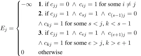
To formalize this new linearity requirement, we elaborate Equation 4 into Equation 10.Ejevaluates
to−∞in three cases. Case 1 is the original coher-ence constraint. Case 2 states that no pointk may
be in the segment with a centre isj, ifklies before the start of the segment (the sequencec(s−1)j = 0,
csj = 1 necessarily corresponds to the start of the
segment). Case 3 handles analogously the end of the segment.
Ej =
−∞ 1. ifcjj = 0 ∧ cij = 1for somei6=j
2. ifcjj = 1 ∧ csj = 1 ∧ c(s−1)j = 0
∧ckj = 1for somes < j,k < s−1
3. ifcjj = 1 ∧ cej = 1 ∧ c(e+1)j = 0
∧ckj = 1for somee > j,k > e+ 1
0 otherwise
(10) TheEfunction nodes are the only changed part of the factor graph, so we only must re-deriveα
mes-sages (availabilities) sent from factorsEto variable nodes. A function-to-variable message is computed as shown in Equation 11 (elaborated Equation 3), and the only incoming messages toEnodes are
re-sponsibilities (ρmessages):
µf→x= max
N(f)\x(f(x1, . . . , xm) + X
x0∈N(f)\x
µx0→f) =
(11)
max
cij, i6=j
((Ej(c1j, . . . , cN j) + X
cij, i6=j
ρij(cij)))
We need to compute the message values for the two possible settings of binary variables – denoted asαij(1)andαij(0)– and propagate the difference
αij =αij(1)-αij(0).
Consider the case of factorEj sending anα
mes-sage to the variable nodecjj (i.e.,i=j). Ifcjj = 0
then pointj is not its own segment centre and the
only valid configuration is to set all othercij to 0:
αjj(0) = max cij,i6=j
(Ej(c1j, . . . , cN j) + X
cij,i6=j
ρij(cij))
(12)
=X
i6=j
ρij(0)
To compute αij(1) (point j is its own segment
centre), we only must maximize over configurations which will not correspond to cases 2 and 3 in Equa-tion 10 (other assignments are trivially non-optimal because they would evaluate Ej to −∞). Let the
start of a segment bes,1 ≤ s < jand the end of
the segment bee,j+ 1< e≤N. We only need to
consider configurations such that all points between
The following picture shows a valid configuration.3
1 s j e N
To compute the messageαij(1), i=j, we have:
αjj(1) = j
max
s=1[
s−1
X
k=1
ρkj(0) + j−1
X
k=s
ρkj(1)]+ (13)
N
max
e=j[ e X
k=j+1
ρkj(1) + N X
k=e+1
ρkj(0)]
Subtracting Equation 12 from Equation 13, we get:
αjj =αjj(1)−αjj(0) = (14)
j
max
s=1(
j−1
X
k=s
ρkj) + N
max
e=j( e X
k=j+1
ρkj)
Now, consider the case of factorEj sending anα
message to a variable node cij other than segment
exemplarj(i.e.,i6=j). Two subcases are possible:
pointimay lie before the segment centrej(i < j),
or it may lie after the segment centre (i > j).
The configurations which may maximize αij(1)
(the message value for setting the hidden variable to 1) necessarily conform to two conditions: point
j is labelled as a segment centre (cjj = 1) and all
points lying between i and j are in the segment.
This corresponds to Equation 15 for i < j and to
Equation 16 fori > j. Pictorial examples of
corre-sponding valid configurations precede the equations.
1 s i j e N
αij, i<j(1) =maxi s=1[
s−1
X
k=1
ρkj(0) + i−1
X
k=s
ρkj(1)]+
(15)
j X
k=i+1
ρkj(1) + N
max
e=j[ e X
k=j+1
ρkj(1) + N X
k=e+1
ρkj(0)]
3Variablesc
ijset to 1 are shown as shaded circles, to 0 – as
white circles. Normally, variables form a column in the factor graph; we transpose them to save space.
1 s j i e N
αij, i>j(1) = j
max
s=1[
s−1
X
k=1
ρkj(0) + j−1
X
k=s
ρkj(1)]+
(16)
i−1
X
k=j
ρkj(1) + N
max
e=i [ e X
k=i+1
ρkj(1) + N X
k=e+1
ρkj(0)]
To compute the message value for setting the hidden variable cij to 0, we again distinguish
betweeni < j andi > j and consider whethercjj
= 1 orcjj = 0 (pointj is / is not a segment centre).
Forcjj = 0 the only optimal configuration iscij = 0
for alli6=j. Forcjj = 1 the set of possible optimal
configurations is determined by the position of point
iwith respect to pointj. Following the same logic
as in the previous cases we get Equation 17 for
i < jand Equation 18 fori > j.
1 i s j e N
αij(0) = max( X
k /∈i,j
ρkj(0), (17)
i−1
X
k=1
ρkj(0) + j
max
s=i+1[
s−1
X
k=i+1
ρkj(0) + j−1
X
k=s
ρkj(1)]+
ρjj(1) + N
max
e=j[ e X
k=j+1
ρkj(1) + N X
k=e+1
ρkj(0)])
1 s j e i N
αij(0) = max( X
k /∈i,j
ρkj(0), (18)
j
max
s=1[
s−1
X
k=1
ρkj(0) + j−1
X
k=s
ρkj(1)]+
ρjj(1) + i−1
max
e=j[ e X
k=j+1
ρkj(1) + i−1
X
k=e+1
ρkj(0)]
N X
k=i+1
ρkj(0))
Algorithm 1Affinity Propagation for Segmentation
1: input: 1) a set of pairwise similarities{SIM(i, j)}(i,j)∈{1,...,N}2,SIM(i, j) ∈R; 2) a set of
prefer-ences (self-similarities){SIM(i, i)}i∈{1,...,N}indicatinga priorilikelihood of pointibeing a segment
centre
2: initialization:∀i, j:αij = 0(set all availabilities to 0)
3: repeat
4: iteratively update responsibilities (ρ) and availabilities (α)
5:
∀i, j:ρij =SIM(i, j) + max
k6=j(SIM(i, k)−αik)
6:
∀i, j:αij = j max
s=1(
j−1
X
k=s
ρkj) + N
max
e=j ( e X
k=j+1
ρkj) ifi=j
min[maxi
s=1
i−1
X
k=s
ρkj + j X
k=i+1
ρkj + N
max
e=j e X
k=j+1
ρkj,
i
max
s=1
i−1
X
k=s
ρkj+ j
min
s=i+1
s−1
X
k=i+1
ρkj] ifi < j
min[maxj
s=1
j−1
X
k=s
ρkj + i−1
X
k=j
ρkj+ N
max
e=i e X
k=i+1
ρkj,
i−1
min
e=j i−1
X
k=e+1
ρkj+ N
max
e=i e X
k=i+1
ρkj] ifi > j
7: untilconvergence
8: compute the final configuration of variables:∀i, j jis the exemplar foriiffρij+αij >0
9: output: exemplar assignments
i > j appear in Algorithm 1, where we summarize
the whole process.
The equations look cumbersome but they are triv-ial to compute. Every summand corresponds to find-ing the most likely start or end of the segment, tak-ing into accountfixedinformation. When computing messages for any given sender node, we can remem-ber the maximizing values for neighbouring recipi-ent nodes. For example, after computing the avail-ability message from factorEj tocij, we must only
consider one more responsibility value when com-puting the message fromEjto variablec(i+1)j. The
cost of computing a message is thus negligible. When the matrix is fully specified, each iteration requires passing 2N2 messages, so the algorithm
runs in O(N2) time and requires O(N2) memory (to store the similarities, the availabilities and the
responsibilities). When performing segmentation, however, the user generally has some idea about the average or maximum segment length. In such more realistic cases, the input matrix of similarities is sparse – it is constructed by sliding a window of size M. M usually needs to be at least twice the
maximum segment length or thrice the average seg-ment length. Each iteration, then, involves sending
2M N messages and the storage requirements are
alsoO(M N).
As is common in loopy belief propagation algo-rithms, both availability and responsibility messages are dampened to avoid overshooting and oscillating. The dampening factor isλwhere0.5≤λ <1.
newM sg=λ∗oldM sg+ (1−λ)newM sg (19)
from a small development set to fine-tune a few pa-rameters: preference values and the dampening fac-tor. APSdoes not require (nor allow) specifying the number of segments beforehand. The granularity of segmentation is adjusted through preference values; this reflect how likely each sentence is to be selected as a segment centre. (This translates into the cost of adding a segment.)
Because each message only requires the knowl-edge about one column or row of the matrix, the al-gorithm can be easily parallelized.
5 Experimental Setting
Datasets. We evaluate the performance of the
APS algorithm on three datasets. The first, com-piled by Malioutov and Barzilay (2006), consists of manually transcribed and segmented lectures on Artificial Intelligence, 3 development files and 19 test files. The second dataset consists of 227 chap-ters from medical textbooks (Eisenstein and Barzi-lay, 2008), 5 of which we use for development. In this dataset the gold standard segment boundaries correspond to section breaks specified by the au-thors. The third dataset consists of 85 works of fic-tion downloaded from Project Gutenberg, 3 of which are used for development. The segment boundaries correspond to chapter breaks or to breaks between individual stories. They were inserted automatically using HTML markup in the downloaded files.
The datasets exhibit different characteristics. The lecture dataset and the fiction dataset are challeng-ing because they are less cohesive than medical text-books. The textbooks are cognitively more difficult to process and the authors rely on repetition of ter-minology to facilitate comprehension. Since lexical repetition is the main source of information for text segmentation, we expect a higher performance on this dataset. Transcribed speech, on the other hand, is considerably less cohesive. The lecturer makes an effort to speak in “plain language” and to be com-prehensible, relying less on terminology. The use of pronouns is very common, as is the use of examples. Repeated use of the same words is also uncom-mon in fiction. In addition, the dataset was compiled automatically using HTML markup. The markup is not always reliable and occasionally the e-book proofreaders skip it altogether, which potentially
adds noise to the dataset.
Baselines. We compare the performance of
APSwith that of two state-of-the-art segmenters: the Minimum Cut segmenter (Malioutov and Barzilay, 2006) and the Bayesian segmenter (Eisenstein and Barzilay, 2008). The authors have made Java imple-mentations publicly available. For the Minimum Cut segmenter, we select the best parameters using the script included with that distribution. The Bayesian segmenter automatically estimates all necessary pa-rameters from the data.
Preprocessing and the choice of similarity met-ric. As described in Section 4, the APS algorithm takes as inputs a matrix of pairwise similarities be-tween sentences in the document and also, for each sentence, a preference value.
This paper focuses on comparing globally in-formed segmentation algorithms, and leaves for fu-ture work the exploration of best similarity metrics. To allow fair comparison, then, we use the same metric as the Minimum Cut segmenter, cosine sim-ilarity. Each sentence is represented as a vector of token-type frequencies. Following (Malioutov and Barzilay, 2006), the frequency vectors are smoothed by adding counts of words from the adjacent sen-tences and then weighted using a tf.idf metric (for details, seeibid.) The similarity between sentence vectorss1ands2is computed as follows:
cos(s1, s2) =
s1•s2
||s1|| × ||s2|| (20) The representation used by the Bayesian segmenter is too different to be incorporated into our model di-rectly, but ultimately it is based on the distribution of unigrams in documents. This is close enough to our representation to allow fair comparison.
The fiction dataset consists of books: novels or collections of short stories. Fiction is known to ex-hibit less lexical cohesion. That is why – when working on this dataset – we work at the paragraph level: the similarity is measured not between sen-tences but between paragraphs. We use this repre-sentation with all three segmenters.
All parameters have been fine-tuned on the devel-opment portions of the datasets. ForAPSalgorithm
BayesSeg MinCutSeg APS
AI 0.443 0.437 0.404
Clinical 0.353 0.382 0.371
[image:9.612.76.299.71.129.2]Fiction 0.377 0.381 0.350
Table 1: Results of segmenting the three datasets us-ing the Bayesian segmenter, the Minimum Cut seg-menter andAPS.
parameters for the similarity metric (best variation of tf.idf, the window size and the decay factor for smoothing) were set using the script provided in the Minimum Cut segmenter’s distribution.
Evaluation metric. We have measured the per-formance of the segmenters with the WindowDiff metric (Pevzner and Hearst, 2002). It is computed by sliding a window through reference and through segmentation output and, at each window position, comparing the number of reference breaks to the number of breaks inserted by the segmenter (hypo-thetical breaks). It is a penalty measure which re-ports the number of windows where the reference and hypothetical breaks do not match, normalized by the total number of windows. In Equation 21,
ref andhypdenote the number of reference and
hy-pothetical segment breaks within a window.
winDif f = 1 N−k
NX−k
i=1
(|ref −hyp| 6= 0) (21)
6 Experimental Results and Discussion Table 1 compares the performance of the three seg-menters using WindowDiff values. On the lecture and fiction datasets, theAPSsegmenter outperforms the others by a small margin, around 8% over the better of the two. It is second-best on the clinical textbook dataset. According to a one-tailed paired t-test with 95% confidence cut-off, the improvement is statistically significant only on the fiction dataset. All datasets are challenging and the baselines are very competitive, so drawing definitive conclusions is difficult. Still, we can be fairly confident that
APSperforms at least as well as the other two seg-menters. It also has certain advantages.
One important difference between APS and the other segmenters is that APS does not require the
number of segments as an input parameter. This is very helpful, because such information is generally unavailable in any realistic deployment setting. The parameters are fine-tuned to maximize WindowDiff values, so this results in high-precision, low-recall segment assignments; that is because WindowDiff favours missing boundaries over near-hits.
APSalso outputs segment centres, thus providing some information about a segment’s topic. We have not evaluated how descriptive the segment centres are; this is left for future work.
APS performs slightly better than the other seg-menters but not by much. We hypothesize that one of the reasons is thatAPS relies on the presence of descriptive segment centres which are not necessar-ily present for large, coarse-grained segments such as chapters in novels. It is possible forAPSto have an advantage performing fine-grained segmentation.
7 Conclusions and Future Work
In this paper we have presentedAPS– a new algo-rithm for linear text segmentation. APS takes into account the global structure of the document and outputs segment boundaries and segment centres. It scales linearly in the number of input sentences, per-forms competitively with the state-of-the-art and is easy to implement. We also provide a Java imple-mentation of theAPSsegmenter.
We consider two main directions for future work: using more informative similarity metrics and mak-ing the process of segmentation hierarchical. We chose to use cosine similarity primarily to allow fair comparison and to judge the algorithm itself, in iso-lation from the information it uses. Cosine similarity is a very simple metric which cannot provide an ad-equate picture of topic fluctuations in documents. It is likely that dictionary-based or corpus-based simi-larity measures would yield a major improvement in performance.
Acknowledgements
We thank Inmar Givoni for explaining the details of binary Affinity Propagation and for comment-ing on our early ideas in this project. Many thanks to Yongyi Mao for a helpful discussion on the use Affinity Propagation for text segmentation.
References
Bishop, Christopher M. 2006. Pattern Recognition and Machine Learning. Springer.
Blei, David and Pedro Moreno. 2001. Topic Segmenta-tion with an Aspect Hidden Markov Model. In Pro-ceedings of the 24th annual international ACM SIGIR conference on Research and development in informa-tion retrieval, pages 343–348. ACM Press.
Blei, David M., Andrew Ng, and Michael Jordan. 2003. Latent Dirichlet allocation. Journal of Machine Learning Research, 3:993–1022.
Choi, Freddy Y. Y. 2000. Advances in Domain Inde-pendent Linear Text Segmentation. InProceedings of NAACL, pages 26–33.
Eisenstein, Jacob and Regina Barzilay. 2008. Bayesian Unsupervised Topic Segmentation. InProceedings of the 2008 Conference on Empirical Methods in Natu-ral Language Processing, pages 334–343, Honolulu, Hawaii, October.
Frey, Brendan J. and Delbert Dueck. 2007. Clustering by Passing Messages Between Data Points. Science, 315:972–976.
Givoni, Inmar E. and Brendan J. Frey. 2009. A Binary Variable Model for Affinity Propagation. Neural Com-putation, 21:1589–1600.
Haghighi, Aria and Lucy Vanderwende. 2009. Explor-ing Content Models for Multi-Document Summariza-tion. InProceedings of Human Language Technolo-gies: The 2009 Annual Conference of the North Ameri-can Chapter of the Association for Computational Lin-guistics, pages 362–370, Boulder, Colorado, June. Hearst, Marti A. 1997. TextTiling: segmenting text into
multi-paragraph subtopic passages. Computational Linguistics, 23:33–64, March.
Kschischang, Frank R., Brendan J. Frey, and Hans-A Loeliger. 2001. Factor graphs and the sum-product algorithm. InIEEE Transactions on Information The-ory, Vol 47, No 2, pages 498–519, February.
Lafferty, John, Andrew McCallum, and Fernando Pereira. 2001. Conditional random fields: Probabilis-tic models for segmenting and labeling sequence data. InProceedings of ICML-01, pages 282–289.
Malioutov, Igor and Regina Barzilay. 2006. Minimum Cut Model for Spoken Lecture Segmentation. In Pro-ceedings of the 21st International Conference on Com-putational Linguistics and 44th Annual Meeting of the Association for Computational Linguistics, pages 25– 32, Sydney, Australia, July.
Misra, Hemant, Franc¸ois Yvon, Joemon M. Jose, and Olivier Capp´e. 2009. Text segmentation via topic modeling: an analytical study. In 18th ACM Con-ference on Information and Knowledge Management, pages 1553–1556.
Oh, Hyo-Jung, Sung Hyon Myaeng, and Myung-Gil Jang. 2007. Semantic passage segmentation based on sentence topics for question answering. Information Sciences, an International Journal, 177:3696–3717, September.
Pearl, Judea. 1982. Reverend Bayes on inference en-gines: A distributed hierarchical approach. In Pro-ceedings of the American Association of Artificial In-telligence National Conference on AI, pages 133–136, Pittsburgh, PA.
Pevzner, Lev and Marti A. Hearst. 2002. A Critique and Improvement of an Evaluation Metric for Text Seg-mentation.Computational Linguistics, 28(1):19–36. Stoyanov, Veselin and Claire Cardie. 2008. Topic
identi-fication for fine-grained opinion analysis. InCOLING ’08 Proceedings of the 22nd International Conference on Computational Linguistics - Volume 1, pages 817– 824.