An Example of Peak Finding in Univariate Data by Least Squares Approximation and Restrictions on the Signs of the First Differences

An Example of Peak Finding in Univariate Data by

Least Squares Approximation and

Restrictions on the Signs of the First Differences

I. C. Demetriou

Abstract—We consider an application of the least squares piecewise monotonic data approximation method to the problem of locating significant extrema in univariate observations that are contaminated by random errors. The piecewise monotonic approximation method makes the smallest change to the data such that the first differences of the smoothed values change sign a prescribed number of times, but the positions of the sign changes are unknowns of the optimization process. We present a numerical example in order to show the efficiency of the method for peak finding. The example is an application to 31959 noisy observations of daily sunspots. Our results suggest some subjects for future research in automatic peak finding.

Index Terms—data smoothing, divided differences, peak find-ing, piecewise monotonic approximation, sunspots

I. BACKGROUND

T

he piecewise monotonic data approximation method by Demetriou and Powell [8] provides useful applications in signal processing (see, for example, [2], [7], [12], [21] and references therein). In this paper an example is worked out as an illustration of the method for estimating turning points of a function from some measurements of its values that contain random errors.

Let {φi : i = 1,2, . . . , n} be a sequence of measured

values of a functionf(x)at the abscissaex1< x2<· · ·<

xn, but the measurements include random errors (noise).

We assume that if the function has turning points, then the number of measurements is substantially greater than the number of turning points. Therefore some algorithms have been developed by [8] and [5] that modify the measurements if their first differences {φi+1 −φi : i = 1,2, . . . , n−1}

include more thank−1sign changes, wherekis a prescribed integer. This condition allows k monotonic sections to the smoothed data, alternately increasing and decreasing. Let

{yi : i = 1,2, . . . , n} be the smoothed values, which we

regard as components of an-vectory.

Specifically, the method calculates a vector y that mini-mizes the sum of squares of the errors

Φ(y) = n X

i=1

(yi−φi)2 (1)

Manuscript received April 16, 2015.

The author is very grateful to two referees for several useful comments on the first draft of this paper. He is also grateful to the Solar Influences Data Analysis Center of the Royal Observatory of Belgium for providing the data set with the sunspots. This work was supported in part by the University of Athens under Research Grant 11105.

I. C. Demetriou is with the Division of Mathematics and Informatics, Department of Economics, University of Athens, 1 Sofokleous and Aristidou street, Athens 10559, Greece (e-mail: [email protected]).

subject to the piecewise monotonicity constraints

ytj−1≤ytj−1+1≤ · · · ≤ytj, ifj is odd

ytj−1≥ytj−1+1≥ · · · ≥ytj, ifj is even

)

, (2)

where the integers {tj : j = 1,2, . . . , k−1}, namely the

positions of theturning points or extrema of the fit, satisfy the conditions

1 =t0≤t1≤ · · · ≤tk =n. (3)

The integers{tj :j = 1,2, . . . , k−1} are not known in

advance and they are variables in the optimization calculation that gives a best fit. This raises the number of combinations of integer variables to the order O(nk_{), but fortunately}

the method of Section II allows an efficient and automatic calculation of an optimal fit y together with the associated integers{tj:j = 1,2, . . . , k−1} in onlyO(kn2)computer

operations. This complexity reduces toO(n)when k= 1or k = 2. Except when k = 1, the problem need not have a unique solution.

The method is suitable for data smoothing when the data errors are so large that they can be detected by the first differences. By contrast, the method may not be suitable if the data contains significant random errors that are too small to cause many sign changes in its first differences. An initial advantage of the method is that it is a projection operator, because if the data satisfy the constraints, then they remain unchanged, so ifP takesφ toy, then P2=P. Further, by considering piecewise linear functions, it is straightforward to see that there exists a piecewise monotonic function

{y(x) : x1≤x≤xn}that interpolates the smoothed values,

so{y(xi) =yi: i= 1,2, . . . , n}.

position finding in P31 spectral analysis. Peak finding is a major problem in signal processing, spectroscopy and chromatography that is supported by computer packages, like PeakFitT M _{and Autosignal}T M _{by Systat Software Inc.,}

computing environments like Matlab and many websites (see, for example, [14]). For presentations of medical uses of proton spectroscopy see [16]. The piecewise monotonic method provides optimal extreme values over the whole sequence of data as it is defined by the constraints (2). However, if the user is only interested in a fairly small region about an extremum, he may well combine the global results of our method with his local analyses.

In order to apply the piecewise monotonicity method to a sequence of data, only the parameter k must be set by the user. Then the method automatically and simultaneously provides the optimal turning points and the best fit. The au-thor has developed the Fortran software package L2WPMA [6], which implements the method of [5], as a version of a method in [8]. It is suitable for processing very large numbers of data in real time. The software package has been tested on a variety of data sets showing a performance that provides in practice far shorter computation times than those indicated in theory.

A value for k may be selected by inspecting the plotted data, or by forming tables of the first differences of the data and checking for sign alterations, or by increasing k until the differences{yi−φi: i= 1,2, . . . , n}seem to be due to

the errors of the data. Prior knowledge about f(x)or about the underlying process may provide estimates ofk, but it is not inefficient to run the algorithm of [8] for a sequence of integers kif a suitable value is not known in advance.

The paper is organized as follows. In Section II we give a brief description of the method with emphasis on properties of the turning points of the smoothed data. In Section III we consider a numerical example in order to illustrate the method. Specifically, we apply the method on 31959 observations of daily sunspots during the time period August 1928 - February 2015, we present some results and we demonstrate the capability of the method in locating turning points. The Karush-Kuhn-Tucker statistical test provided an adequate value ofk automatically. In Section IV we present some concluding remarks and discuss on the possibility of future directions of this research.

II. SOMEFEATURES OF THEPIECEWISEMONOTONIC APPROXIMATIONMETHOD

This section gives some details of the method that are needed in the application of Section III. For proofs one may consult the references stated previously.

Turning points are important to this calculation, because they have properties that are used in practice and enhance the computation greatly. In order to state these properties, we definet∈[1, n] to be the index of a local minimum of the data if, moving to the left or right fromφt in the sequence {φi : i = 1,2, . . . , n}, we find either φi > φt or the end

of the sequence before φi < φt occurs, and analogously

for a local maximum. We denote the sets of the indices of local minima and local maxima of the data by L and U

respectively. We note thatL andU can be formed inO(n)

operations, each of these sets has fewer than n/2 elements

that are in strictly ascending order and their interior elements interlace.

If the number of extrema in the data is less thank−1, then y = φ, because in this case φ satisfies the piecewise monotonicity constraints. If, however,φdoes not satisfy the piecewise monotonicity constraints, as it occurs in practice, then it is proved that the turning point indices {tj : j = 1,2, . . . , k−1} of a best fit y are all different and at the turning points we have the interpolation conditions

ytj =φtj, j= 1,2, . . . , k−1. (4)

The component ytj, for some j ∈ [1, k −1], need not be

where max{φi: tj−1≤i≤tj+1}occurs. Indeed, an

exam-ple in [6] considers the datan= 5,xi =i, i= 1,2, . . . ,5

and, φ1 = φ2 = 2, φ3 = −7, φ4 = 3 and φ5 = −5,

whereφ4 =max{φi : 1 ≤i ≤5}. Then the example finds

that the components of a monotonic increasing / decreasing fit z subject to the condition that its maximum is at the fourth data point satisfy z1 = z2 = z3 = −1, z4 = 3

andz5 =−5 and give Φ(z) = 54. Further, the optimal fit

y∗ with two monotonic sections in (2) has the components y₁∗ = y∗₂ = 2, y∗₃ = y₄∗ = −2 and y₅∗ = −5 and gives

Φ(y∗) = 50<Φ(z) = 54. However, the maximum is at the first or at the second data point, different from the fourth where max{φi: 1≤i≤5} occurs.

In view of the inequalities

(

ytj−1≤ytj ≥ytj+1, if j is odd

ytj−1≥ytj ≤ytj+1, if j is even

(5)

and (4), we see that the constraintsytj−1 ≤ytj andytj ≥

ytj+1 if j is odd, and analogously if j is even, need not be

considered in the calculation of an optimal fit. Thus, each monotonic section in a best piecewise monotonic fit is the optimal fit itself to the corresponding data. Hence it can be obtained by a separate calculation and the components{yi:

i=tj−1, tj−1+ 1, . . . , tj} on[xtj−1, xtj]minimize the sum

of the squares

tj

X

i=tj−1

(yi−φi)2 (6)

subject to the constraints

yi≤yi+1, i=tj−1, . . . , tj−1, ifj is odd (7)

or subject to the constraints

yi≥yi+1, i=tj−1, . . . , tj−1, if j is even. (8)

In the former case the sequence {yi : i = tj−1, tj−1 + 1, . . . , tj} is the best monotonic increasing fit to {φi :i =

tj−1, tj−1+ 1, . . . , tj} and in the latter case the best

mono-tonic decreasing one. The statement suggests expressing (1) in the form

Φ(y) =α(t0, t1) +β(t1, t2) +α(t2, t3) +· · ·+δ(tk−1, tk),

where, for positive integerspandqsuch that1≤p≤q≤n, we define

α(p, q) = min

yp≤yp+1≤···≤yq

q X

i=p

and

β(p, q) = min

yp≥yp+1≥···≥yq

q X

i=p

(yi−φi)2 (10)

and δ denotes α if k is odd and β if k is even. The computation of all {α(p, i) : i = p, p+ 1, . . . , q} with the best fit that occurs in (9) is achieved in only O(q−p)

computer operations and similarly for the β’s.

Further, the required piecewise monotonic fit is obtained by a dynamic programming formula that makes use of the separation property of its components. We defineY(k, n)to be the set ofn-vectorsythat satisfy the constraints (2). Then the first tk−1 components of an optimal y in Y(k, n) give

an optimal fit fromY(k−1, tk−1)toφi,i= 1,2, . . . , tk−1

and the last n−tk−1 components give the optimal fit to the

remaining data subject to the constraintsytk−1 ≤ytk−1+1≤ · · · ≤ytk, if kis odd, or subject to the constraintsytk−1 ≥

ytk−1+1≥ · · · ≥ytk, ifkis even. For any integersm∈[1, k]

andt∈[1, n], we define

γ(m, t) = min

z∈Y(m,t)

t X

i=1

(zi−φi)2,

where Y(m, t) is the set of t-vectors with m monotonic sections analogously toY(k, n). Thereforetk−1 satisfies the

equation

γ(k−1, tk−1) +α(tk−1, n) =

min

1≤s≤n[γ(k−1, s) +α(s, n)], ifk is odd

γ(k−1, tk−1) +β(tk−1, n) =

min

1≤s≤n[γ(k−1, s) +β(s, n)], ifkis even. 

       

       

(11)

It follows that the least value of the right hand side of (11) can be found inO(n)computer operations provided that the sequences{γ(k−1, s) : s= 1,2, . . . , n}and{α(s, n) : s= 1,2, . . . , n} or{β(s, n) : s= 1,2, . . . , n}are available.

Therefore in order to calculateγ(k, n), which is the least value of (1), we begin the calculation fromγ(1, t) =α(1, t), for t = 1,2, . . . , n, and proceed by applying the dynamic programming formulae

γ(m, t) = 



 min

1≤s≤t[γ(m−1, s) +α(s, t)], modd

min

1≤s≤t[γ(m−1, s) +β(s, t)], meven,

(12) for t = 1,2, . . . , n, for every value of m∈[2, k]. We store alsoτ(m, t), namely the value ofsthat minimizes expression (12), for each value ofm andt.

At the end of the process m = k occurs and the value τ(k, n)is the integertk−1 that is required in equation (11).

Then, because τ(k−1, tk−1) is the optimal value of s in

expression (12) when m = k−1 and t = tk−1, it is the

required value tk−2. Hence, we set tk = n and we obtain

the sequence of optimal values{tj: j= 1,2, . . . , k−1}by

the backward formula

tm−1=τ(m, tm), for m=k, k−1, . . . ,2. (13)

Accordingly, the components of an optimal fit are monotonic increasing on[1, t1]and on[tj, tj+1]for evenjin[1, k−1]

and monotonic decreasing on[tj, tj+1]for oddjin[1, k−1].

This dynamic programming process requires O(kn2₎

com-puter operations.

Formulae (12) provide the basis for the calculation, but far more efficient formulae are employed in practice. In-deed, we assume in this calculation that φ 6∈ Y(k, n)

and let {t1, t2, . . . , tk−1} be optimal integers. If t = t`

for some ` ∈ {2,3, . . . , k − 1} such that φt+1 = φt,

then{t1, t2, . . . , t`−1, t`+1, t`+1. . . , tk−1}are also optimal.

Hence, it is not necessary to compute both γ(m, t) and γ(m, t+ 1) and in fact the integertm−1 =τ(m, tm) is the

index of a local maximum of the data if m is even, that is tm−1∈ U, and it the index of a local minimum ifmis odd,

that istm−1∈ L. Further, if the righthand side of (12) is least

for somes < t, thenssatisfies similar conditions. Therefore we only need to compute γ(m, t) when t is the index of a local extremum of the data and similarly for s. With these choices, the process requiresO(n|U |+k|U |2_)computer

operations, which provides a considerable operations saving in practice. More improvements of the calculation are avail-able in [8] and [5], which are summarized by our software package L2WPMA [6].

In Section III we apply a version of L2WPMA that calculates initially an optimal fit with k = 2 monotonic sections and then an iterative procedure is started. On each iteration an optimal fit with k+ 2 monotonic sections is calculated, say it isy˜, and then it is tested if y˜is improved with respect to the fit withkmonotonic sections, say it isy, on each interval [xtj−1, xtj]. If the test is affirmative then

k is increased by 2 and another iteration is commenced. Otherwise y is accepted as an adequate approximation to the data. The test for whether the fit need be improved is based on the value of the Karush-Kuhn-Tucker (Lagrange multiplier) statistic (see, for example, [15]) that employs the components ofy and the components of y˜. We accepted y˜

for values of the Karush-Kuhn-Tucker test that were larger than the associated0.1% value of the F-distribution.

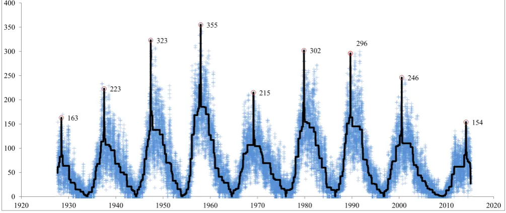
III. NUMERICALEXAMPLE INPEAKFINDING OFDAILY SUNSPOTSDURING1927 - 2015

In order to illustrate the efficacy of our method for identifying important extrema in noisy data, we present a numerical example which considers 31959 data points that span the period from August 1927 to February 2015 of the daily sunspot numbers. These numbers show dark spots that appear periodically on the solar surface and affect terrestrial magnetism and other terrestrial phenomena [17], [18]. The datafile dayssnv0-1.dat was downloaded from the website of the Solar Influences Data Analysis Center (SIDC) of the Royal Observatory of Belgium [19]. The datafile contains individual yearly data of the daily sunspot number in three columns: The first column keeps year, month and day, the second column keeps year and fraction of year (in Julian years of 365.25 days) and, the third column keeps the sunspot number. The second and third column provided the data pairs

(xi, φi), which we plot in Fig. 1. The total number of local

minima of the data is |L| = 6064 and the total number of local maxima is |U | = 6063. We see that the data vary considerably and exhibit cycles and spikes.

163

223

323

355

215

302

296

246

154

0 50 100 150 200 250 300 350 400

[image:4.595.47.550.62.274.2]

1920 1930 1940 1950 1960 1970 1980 1990 2000 2010 2020

Fig. 1. Detected peaks (circles) by best piecewise monotonic fit withk= 18to 31959 daily sunspots (plus signs) during 1927 - 2015. The solid line illustrates the best fit. The numbers give the sunspots at the corresponding dates.

TABLE I

LEFT FIVE COLUMNS: TURNING POINTS IN DAILY SUNSPOTS DURING1927 - 2015BY A BEST FIT WITHk= 18MONOTONIC SECTIONS. RIGHT EIGHT COLUMNS: THE TURNING POINTS POSITION OF THE OPTIMAL FIT FORk= 2,4, . . . ,16ARE INDICATED BY THE TIMES SIGN

j tj Date Year (xt_j) Sunspot number (φt_j) k= 2 4 6 8 10 12 14 16

0 1 19270831 1927.663 56 × × × × × × × ×

1 300 19280625 1928.482 163

2 2259 19331105 1933.845 0

3 3604 19370712 1937.528 223 × ×

4 6076 19440418 1944.296 0 × ×

5 7208 19470525 1947.395 323 × × × × ×

6 9632 19540112 1954.031 0 × × × × ×

7 11074 19571224 1957.979 355 × × × × × × × ×

8 13473 19640719 1964.548 0 × × ×

9 15154 19690224 1969.150 215 × × ×

10 17651 19751227 1975.986 0 × × × × × × ×

11 19065 19791110 1979.858 302 × × × × × × ×

12 21485 19860626 1986.483 0 × × × × × ×

13 22656 19890909 1989.689 296 × × × × × ×

14 25217 19960913 1996.701 0 × × × ×

15 26622 20000719 2000.548 246 × × × ×

16 29821 20090422 2009.306 0 ×

17 31593 20140227 2014.157 154 ×

18 31959 20150228 2015.159 41 × × × × × × × ×

with the Karush-Kuhn-Tucker (Lagrange) multiplier test for the automatic determination of k.

The data φ were fed to the program and the best fit

with k= 18 monotonic sections was calculated. Hence the method detected 17 turning points, which gives 9 peaks. In the left part of Table I we present the turning point indices

{t1, t2, . . . , t17} as well as t0 = 1 and t18 = 31959, the

associated sunspot date according to the format year, month and day, the year in decimal form and the sunspot number; the odd turning point indices indicate the peaks and the even ones indicate the troughs. Fig. 1 displays the fit and the detected peaks. Indeed, the fit to the data is much smoother than are the data values themselves, it has revealed turning points that seem to be adequately located and it has followed the in-between the turning points trends.

In the right part of Table I we indicate the positions of the turning points of each optimal fit for k = 2,4, . . . ,16

in correspondence with the column labeled “tj” derived

when k = 18. For example, when k = 4 the turning

points occur at the positions 11074, 17651 and 19065 as indicated by the times signs in the column labeled “4”. We remind that as k was increased by 2, all the turning points were found automatically by the method. The method iterated until the Karush-Kuhn-Tucker test indicated no need for further improvement of the fit. We see that the extra turning points of the optimal approximation with k + 2

monotonic sections occur between adjacent turning points of the optimal approximation with k monotonic sections. Although it is noticeable that the turning points of the optimal approximation with k monotonic sections are preserved by the optimal approximation with k+ 2 monotonic sections, any algorithm based on local improvements of an optimal approximation withk monotonic sections cannot succeed in finding more than a local minimum of (1), which may not be a global minimum [4].

[image:4.595.96.501.349.533.2]

val-TABLE II

DAILY SUNSPOTS AND SMOOTHED DATA DURING20131009-20140518

20131009 79 79.00 20131115 113 85.80 20131222 83 86.52 20140128 54 86.52 20140306 91 93.50 20140412 55 91.76 20131010 90 85.80 20131116 125 85.80 20131223 81 86.52 20140129 66 86.52 20140307 96 93.50 20140413 60 91.76 20131011 91 85.80 20131117 131 85.80 20131224 79 86.52 20140130 69 86.52 20140308 83 91.76 20140414 79 91.76 20131012 84 85.80 20131118 99 85.80 20131225 70 86.52 20140131 65 86.52 20140309 79 91.76 20140415 109 91.76 20131013 99 85.80 20131119 77 85.80 20131226 75 86.52 20140201 66 86.52 20140310 81 91.76 20140416 141 91.76 20131014 96 85.80 20131120 57 85.80 20131227 77 86.52 20140202 83 86.52 20140311 79 91.76 20140417 150 91.76 20131015 96 85.80 20131121 49 85.80 20131228 73 86.52 20140203 89 89.00 20140312 94 91.76 20140418 134 91.76 20131016 89 85.80 20131122 46 85.80 20131229 90 86.52 20140204 101 97.28 20140313 80 91.76 20140419 134 91.76 20131017 109 85.80 20131123 42 85.80 20131230 73 86.52 20140205 117 97.28 20140314 78 91.76 20140420 130 91.76 20131018 116 85.80 20131124 49 85.80 20131231 99 86.52 20140206 120 97.28 20140315 79 91.76 20140421 113 91.76 20131019 97 85.80 20131125 27 85.80 20140101 87 86.52 20140207 103 97.28 20140316 87 91.76 20140422 93 91.76 20131020 85 85.80 20131126 25 85.80 20140102 93 86.52 20140208 103 97.28 20140317 90 91.76 20140423 64 79.31 20131021 96 85.80 20131127 50 85.80 20140103 107 86.52 20140209 103 97.28 20140318 97 91.76 20140424 54 79.31 20131022 88 85.80 20131128 72 85.80 20140104 95 86.52 20140210 96 97.28 20140319 101 91.76 20140425 43 79.31 20131023 93 85.80 20131129 67 85.80 20140105 94 86.52 20140211 111 97.28 20140320 99 91.76 20140426 34 79.31 20131024 108 85.80 20131130 65 85.80 20140106 117 86.52 20140212 113 97.28 20140321 90 91.76 20140427 58 79.31 20131025 103 85.80 20131201 90 85.80 20140107 98 86.52 20140213 103 97.28 20140322 104 91.76 20140428 60 79.31 20131026 99 85.80 20131202 101 85.80 20140108 75 86.52 20140214 91 97.28 20140323 108 91.76 20140429 58 79.31 20131027 111 85.80 20131203 80 85.80 20140109 84 86.52 20140215 79 97.28 20140324 98 91.76 20140430 62 79.31 20131028 110 85.80 20131204 85 85.80 20140110 96 86.52 20140216 72 97.28 20140325 97 91.76 20140501 59 79.31 20131029 112 85.80 20131205 80 85.80 20140111 99 86.52 20140217 74 97.28 20140326 80 91.76 20140502 77 79.31 20131030 109 85.80 20131206 71 85.80 20140112 93 86.52 20140218 89 97.28 20140327 82 91.76 20140503 82 79.31 20131031 97 85.80 20131207 65 85.80 20140113 82 86.52 20140219 88 97.28 20140328 87 91.76 20140504 85 79.31 20131101 72 85.80 20131208 69 85.80 20140114 67 86.52 20140220 93 97.28 20140329 84 91.76 20140505 95 79.31 20131102 69 85.80 20131209 103 86.52 20140115 65 86.52 20140221 95 97.28 20140330 72 91.76 20140506 99 79.31 20131103 84 85.80 20131210 136 86.52 20140116 56 86.52 20140222 102 102.00 20140331 84 91.76 20140507 80 79.31 20131104 87 85.80 20131211 128 86.52 20140117 52 86.52 20140223 111 109.00 20140401 72 91.76 20140508 88 79.31 20131105 83 85.80 20131212 110 86.52 20140118 81 86.52 20140224 107 109.00 20140402 86 91.76 20140509 93 79.31 20131106 99 85.80 20131213 105 86.52 20140119 77 86.52 20140225 120 120.00 20140403 100 91.76 20140510 82 79.31 20131107 113 85.80 20131214 98 86.52 20140120 93 86.52 20140226 145 145.00 20140404 119 91.76 20140511 100 79.31 20131108 97 85.80 20131215 98 86.52 20140121 90 86.52 20140227 154 154.00 20140405 102 91.76 20140512 103 79.31 20131109 71 85.80 20131216 83 86.52 20140122 108 86.52 20140228 137 137.00 20140406 91 91.76 20140513 89 79.31 20131110 69 85.80 20131217 88 86.52 20140123 102 86.52 20140301 111 113.00 20140407 86 91.76 20140514 111 79.31 20131111 77 85.80 20131218 102 86.52 20140124 81 86.52 20140302 113 113.00 20140408 88 91.76 20140515 104 79.31 20131112 92 85.80 20131219 102 86.52 20140125 70 86.52 20140303 115 113.00 20140409 71 91.76 20140516 89 79.31 20131113 104 85.80 20131220 104 86.52 20140126 68 86.52 20140304 101 105.50 20140410 49 91.76 20140517 101 79.31 20131114 118 85.80 20131221 102 86.52 20140127 53 86.52 20140305 110 105.50 20140411 46 91.76 20140518 92 79.31

154

0 20 40 60 80 100 120 140 160 180

20131009 20131019 20131029 20131108 20131118 20131128 20131208 20131218 20131228 20140107 20140117 20140127 20140206 20140216 20140226 20140308 20140318 20140328 20140407 20140417 20140427 20140507 20140517

Fig. 2. Plot of the daily sunspots (plus signs) and the smoothed data (solid line) during 20131009-20140518, which are presented in Table II. Number 154 gives the sunspots on date 20140227.

ues. Specifically, in Table II we display 222 data and solution components around the rightmost turning point integer t17,

which span the time period 20131009-20140518. Index t17

occurs at the date 20140227 which is associated to the value yt17 = 154(it is typed with bold characters in Table II). Of

course, at the peak we have the equationyt17 =φt17 = 154.

The data are presented in six triples of columns, where the first column of each triple keeps the dates, the second column keeps the sunspot numbers and the 3rd column keeps the smoothed values. Further, the smoothed values consist of the monotonic increasing components, which are part of the best monotonic increasing fit on [xt16, xt17], and the

best monotonic decreasing components on [xt17, xn]. Fig.

2 displays the data of Table II. In order to simplify the

discussion, let {s, s+ 1, . . . , t17} be the data indices of the

monotonic section on 20131009-20140227 and we note that the extracted components{ys, ys+1, . . . , yt17} from the best

fit on [x1, xn]give the best monotonic increasing fit to the

data{φs, φs+1, . . . , φt17}. Now, we see that each monotonic

section consists of values of equal components and there are breakpoints r ∈ [s, t17] such that yr < yr+1. If r and `

are any integers in [s, t17] such that yr < yr+1 = yr+2 = · · ·=y`< y`+1, then it is a consequence of the first order

conditions (see, for example, [9]) of minimizing the function

` X

i=r+1

(yi−φi)2

subject to the equality constraints

yr+1=yr+2=· · ·=y`

that the solution satisfies the equations

yr+1=· · ·=y`= 1

`−r

` X

i=r+1

φi.

Hence y` is the best least squares approximation by a

constant to the data {φr+1, φk+2, . . . , φ`} and in general

the values of the equal components in a best monotonic fit are averages of consecutive data. In Table II, we see that the monotonic increasing fit contains the components

{79×1,85.8×60,86.52×56,89×1,97.28×18,102× 1,109×2,120×1,145×1,154×1}, where79×1,85.8×60

of equal components between breakpoints. An important consequence of the breakpoints is that the fit has flexibility in following monotonic data trends.

IV. CONCLUDINGREMARKS

We have presented an application that shows the effective-ness of the piecewise monotonic approximation method in identifying important extrema in discrete noisy data. Piece-wise monotonic approximation as a data smoothing approach can have many applications, because piecewise monotonicity is a property that occurs in a wide range of underlying functions. Despite the large number of local minima that can occur in this optimization calculation, it obtains a global solution in quadratic complexity with respect to n, but in practice the complexity is far lower because the dynamic programming algorithm takes account of several properties of the turning points that reduce the numerical work. The accompanying Fortran software L2WPMA would be the most useful for real time processing applications, because it is user friendly, it does not need user intervention, it is able to process fast and effectively large data sets and provided that k is known it identifies the data extrema automatically. A question that deserves further study is the development of techniques of choosing automatically a value for k. The method of [20], which employs the trend test of [13], is a step towards this direction and worked successfully on a number of examples. Further, the Karush-Kuhn-Tucker test that we employed in Section II seems promising, but more work is needed to gain experience.

The example with the 31959 sunspots data is especially challenging, because the very many peaks that occur in the data raise the number of combinations for optimal extrema to about606417_{/17!. Nonetheless, the least value of (1) was}

reached automatically in negligible time on a common pc. This example drew attention to the effectiveness and accu-racy of L2WPMA at finding the integers{t1, t2, . . . , tk−1}.

Indeed, the number of peaks and their positions in the data sequence show that the results accord with human judgment, while no assumption on any structure of the sunspots data was made. However, some data, as for instance in NMR spec-troscopy [10], have typical structures concerning the number of peaks. Therefore an interesting question for further study is whether theO(n|U |+k|U |2_{)complexity of our method is}

too high for problems involving such data sets. These studies may be helped by solving particular peak finding problems, in order to receive guidance from both underlying structures and numerical results.

REFERENCES

[1] C. de Boor,A Practical Guide to Splines, Revised Edition, NY: Springer-Verlag, Applied Mathematical Sciences, vol. 27, 2001.

[2] A. P. Bruner, K. Scott, D. Wilson, B. Underhill, T. Lyles, C. Stopka, R. Ballinger and E. A. Geiser, “Automatic Peak Finding of Dynamic Batch Sets of Low SNR In-Vivo Phosphorus NMR Spectra”, unpublished manuscript, Departments of Radiology, Physics, Nuclear and Radiolog-ical Sciences, Surgery, Mathematics, Medicine, and Exercise and Sport Sciences, University of Florida, and the Veterans Affairs Medical Cen-ter, Gainesville, Florida, U. S. Available online: cds.ismrm.org/ismrm-1998/.../P1857.PDF (accessed on 21 March 2015)

[3] W. Cheney and W. Light, A Course in Approximation Theory, NY: Brooks/Cole Publishing Company, An International Thompson Publish-ing Company, 2000.

[4] I. C. Demetriou, Data Smoothing by Piecewise Monotonic Divided Differences, Ph.D. Dissertation, Department of Applied Mathematics and Theoretical Physiscs, University of Cambridge, Cambridge, 1985. [5] I. C. Demetriou, “Discrete piecewise monotonic approximation by a

strictly convex distance function”, Mathematics of Computation, vol. 64, 209, pp. 157-180, 1995.

[6] I. C. Demetriou, “Algorithm 863: L2WPMA, a Fortran 77 package for weighted least-squares piecewise monotonic data approximation”,ACM Trans. Math. Softw., vol. 33, 1, pp. 1-19, 2007.

[7] I. C. Demetriou and V. Koutoulidis, “On Signal Restoration by Piece-wise Monotonic Data Approximation”, in Lecture Notes in Engineering and Computer Science: Proceedings of The World Congress on Engi-neering 2013, Eds. S. I. Ao, L. Gelman, D. W. L. Hukins, A. Hunter, A. M. Korsunsky, U.K., 3-5 July, 2013, London, pp. 268-273. [8] I. C. Demetriou and M. J. D. Powell, “Least squares smoothing of

univariate data to achieve piecewise monotonicity”,IMA J. of Numerical Analysis, vol. 11, pp. 411-432, 1991.

[9] R. Fletcher,Practical Methods of Optimization, Chichester, U. K.: J. Wiley and Sons, 2003.

[10] H. Gunther, NMR Spectroscopy: Basic Principles, Concepts and Applications in Chemistry, 3rd ed., Chichester, U. K.: J. Wiley and Sons, 2013.

[11] W. H¨ardle, M. M¨uller, S. Sperlich and A. Werwatz,Nonparametric and Semiparametric Models, Heidelberg, Germany: Springer-Verlag, 2004. [12] J. Lu, “Signal restoration with controlled piecewise monotonicity constraint”, Proceedings of the IEEE International Conference on Acoustics, Speech and Signal Processing, 12 May 1998-15 May 1998, Seattle WA, vol. 3, pp. 1621 - 1624, 1998.

[13] M. J. D. Powell, “Curve fitting by splines in one variable”, in

Numerical Approximation to Functions and Data, ed. J. G. Hayes, The Institute of Mathematics and its Applications, London, U. K.: The Athlone Press, pp. 65 - 83, 1970.

[14] Peak Finding and Measurement. Available online: http://terpconnect. umd.edu/∼toh/spectrum/PeakFindingandMeasurement.htm (accessed on 21 March 2015).

[15] T. Robertson, F. T. Wright and R. L. Dykstra, Order Restricted Statistical Inference, New York: John Wiley and Sons, 1988. [16] V. M. Runge, W. R. Nitz and S. H. Schmeets,The Physics of Clinical

MR Taught Through Images, 2nd ed., New York: Thieme, 2009. [17] F. Scholkmann, J. Boss and M. Wolf, “An Efficient Algorithm for

Au-tomatic Peak Detection in Noisy Periodic and Quasi-Periodic Signals”,

Algorithms, vol. 5, pp. 588-603, 2012.

[18] S. K. Solanki, “Sunspots: An overview”, Astronomy Astrophysics Review, vol. 11, pp. 153-286, 2003.

[19] Solar Influences Data Analysis Center (SIDC) of the Royal Ob-servatory of Belgium. Available online: http://sidc.oma.be/DATA, dayssnv0.dat (accessed on 21 March 2015).

[20] E. Vassiliou and I. C. Demetriou, “An adaptive algorithm for least squares piecewise monotonic data fitting”,Computational Statistics and Data Analysis, vol. 49, pp. 591-609, 2005