A Spectral Method in Time for Initial-Value Problems
Jan Scheffel
Division of Fusion Plasma Physics, Association EURATOM-VR, Alfvén Laboratory, School of Electrical Engineering, KTH Royal Institute of Technology, Stockholm, Sweden
Email: [email protected]
Received April 27, 2012; revised June 22, 2012; accepted June 29, 2012
ABSTRACT
A time-spectral method for solution of initial value partial differential equations is outlined. Multivariate Chebyshev series are used to represent all temporal, spatial and physical parameter domains in this generalized weighted residual method (GWRM). The approximate solutions obtained are thus analytical, finite order multivariate polynomials. The method avoids time step limitations. To determine the spectral coefficients, a system of algebraic equations is solved iteratively. A root solver, with excellent global convergence properties, has been developed. Accuracy and efficiency are controlled by the number of included Chebyshev modes and by use of temporal and spatial subdomains. As exam- ples of advanced application, stability problems within ideal and resistive magnetohydrodynamics (MHD) are solved. To introduce the method, solutions to a stiff ordinary differential equation are demonstrated and discussed. Subse- quently, the GWRM is applied to the Burger and forced wave equations. Comparisons with the explicit Lax-Wendroff and implicit Crank-Nicolson finite difference methods show that the method is accurate and efficient. Thus the method shows potential for advanced initial value problems in fluid mechanics and MHD.
Keywords: Initial-Value Problem; WRM; Time-Spectral; Spectral Method; Chebyshev Polynomial; Fluid Mechanics; MHD
1. Introduction
Initial-value problems are traditionally solved numeri- cally, using finite steps for the temporal domain. The time steps of explicit time advance methods are chosen sufficiently small to be compatible with constraints such as the Courant-Friedrich-Lewy (CFL) condition [1]. Im- plicit schemes may use larger time steps at the price of performing matrix operations at each of these. Semi- implicit methods [2,3] allow large time steps and more efficient matrix inversions than those of implicit methods, but may feature limited accuracy. These methods never- theless provide sufficiently efficient and accurate solu- tions for most applications. For applications in physics where there exist several separated time scales, however, the numerical work relating to advancement in the time domain can become very demanding. Another computa- tional issue is that it may be advantageous to determine parametrical dependences without performing a sequence of runs for different choices of parameter values.
We here outline a fully spectral method for computing semi-analytical solutions of initial-value partial different- tial equations [4]. To this end all time, space and physical parameter domains are treated spectrally, using series expansion. By semi-analytical is meant that approximate solutions are obtained as finite, analytical spectral Cheby-
shev expansions with numerical coefficients. Important applications are scaling studies, in which the detailed parametrical dependence preferably should be estimated in analytical form. Here the envelope of the characteristic dynamics may often be of higher interest than, for exam- ple, fine scale turbulent phenomena. Thus the possibility to filter out, or average, fine structures to obtain higher computational efficiency is a main theme of this work. However, the GWRM may also provide high accuracy when modelling more detailed phenomena. In all cases, the resulting functional solutions are immediately avail- able for differentiation, integration or other analytic sub- sequent usage.
particular importance for “smearing out” small scale fluctuations.
A number of authors have investigated various aspects of spectral methods in time. Some early ideas were not developed further in [7]. In 1986, Tal-Ezer [8,9] pro- posed time-spectral methods for linear hyperbolic and parabolic equations using a polynomial approximation of the evolution operator in a Chebyshev least square sense. Later, Ierley et al. [10] solved a a class of nonlinear para- bolic partial differential equations with periodic bound- ary conditions using a Fourier representation in space and a Chebyshev representation in time. Tang et al. [11] also used a spatial Fourier representation for solution of parabolic equations, but introduced Legendre Petrov- Galerkin methods for the temporal domain. More re- cently Dehghan et al. [12] found solutions to the non- linear Schrödinger equation, using a pseudo-spectral method where the basis functions in time and space were constructed as a set of Lagrange interpolants.
Chebyshev polynomials are used here for the spectral representation in the GWRM. These have several desir- able qualities. They converge rapidly to the approxi- mated function, they are real and can easily be converted to ordinary polynomials and vice versa, their minimax property guarantees that they are the most economical polynomial representation, they can be used for non- periodic boundary conditions (being problematic for Fourier representations) and they are particularly apt for representing boundary layers where their extrema are locally dense [13,14]. The GWRM is fully spectral; all calculations are carried out in spectral space. The pow- erful minimax property of the Chebyshev polynomials [14] implies that the most accurate n-m order approxima- tion to an nth order approximation of a function is a sim- ple truncation of the terms of order > n-m. Thus nonlin- ear products are easily and efficiently computed in spec- tral space. Since the GWRM efficiently uses rapidly convergent Chebyshev polynomial representation for all time, space and parametrical dimensions, pseudospectral implementation [13] has so far not been pursued. The GWRM eliminates time stepping and associated, limiting grid causality conditions such as the CFL condition.
The method is acausal, since the time dependence is calculated by a global minimization procedure acting on the time integrated problem. Recall that in standard WRM methods, initial value problems are transformed into a set of coupled ordinary, linear or non-linear, dif-ferential equations for the time-dependent expansion coefficients. These are solved using finite differencing techniques.
The structure of the paper is as follows. First, the GWRM is outlined mathematically. We show, in Sec-tions 2-4, how integration, differentiation, nonlinearities, as well as initial and boundary conditions are handled in
multivariate Chebyshev spectral space for arbitrary solu- tion intervals. Having transformed the initial-value prob- lem, a set of algebraic equations for the coefficients of the Chebyshev expansions result. These are solved using a new, efficient global nonlinear equation solver which is briefly described in Section 5. The introduction of tem- poral and spatial subdomains, for increasing efficiency, is discussed in Section 6. As an introductory example, we solve a stiff, time-dependent ordinary differential equa- tion representing flame propagation. For studying accu- racy, the nonlinear Burger equation and its exact solution is used. Detailed comparisons with the time differencing Lax-Wendroff (explicit) and Crank-Nicolson methods (semi-implicit) are presented in Section 7. A forced wave equation is subsequently used for studying strongly separated time scales. Finally, we demonstrate applica- tion of the GWRM to stability problems formulated within the linearised ideal and resistive magnetohydro- dynamic (MHD) models. The paper ends with a sum- mary and conclusions.
2. Generalized Weighted Residual Method
2.1. MethodConsider a system of parabolic or hyperbolic initial-value partial differential equations, symbolically written as
D f
t
u u (1)
where u u
t, ;x p
is the solution vector, D is a linear or nonlinear matrix operator and is an explicitly given source (or forcing) term. Note that Dmay depend on both physical variables (t, x and u) and physical parameters (denoted p) and that f is assumed arbitrary but non-dependent on u. Initial u(t0, x; p) as
well as (Dirichlet, Neumann or Robin) boundary u(t, xB;
p) conditions are assumed known.
, ; f f t x p
Our aim is to determine a spectral solution of Equation (1), using Chebyshev polynomials [14] in all dimensions. To avoid inverting a matrix solution vector, associated with the time derivative, Equation (1) is now integrated in time. The resulting formulation of the problem is con- veniently coupled to the fixed point algebraic equation solver SIR described in Section 5. Thus
0
0
, ; , ;
, ; , ; d
t
t
t t
D t f t t
u x p u x p
u x p x p (2)
can be written as real, simple polynomials of degree n
and are orthogonal in the interval
1,1
x over a weight. Thus , 1 ,
2
1/21x T x0
1 T x
22 2 1
T x x
T Pmetc. For simplicity, we will now restrict the discussion to a single equation with one spatial dimension x and one physical parameter p. Schemes for several coupled equa- tions and higher dimensions may subsequently be straightforwardly obtained. Thus,
, ;x p
Tl 0 0 0 K L M
k l m
a Tklm k
u t (3)
with
, , p
t Ax P
t x x B B p B p A
t A
(4) and Az
z1z0
2, z
1 0
. Here z = t, x or p.Indices “0” and “1” denote lower and upper computa- tional domain boundaries, respectively. The basic Che- byshev polynomials have the limited range of variation
2 B z z
1,1
and they require arguments within the same range. The variables , and P used here allow for arbitrary, finite computational domains. We note that, at the spatial boundaries,
x0 1 and
x1 1 .Primes on summation signs in Equation (3) indicate that each occurence of a zero coefficient index should render a multiplicative factor of 1/2.
Next, we use a weighted residual formulation in order to determine the unknown coefficients aklm of the solu- tion ansatz (3).
2.2. Spectral Coefficients from Weighted Residual Method
The weighted residual method (WRM) is based on the idea that a residual, when using the ansatz (3) in Equa- tion (2), is to be minimized globally. The residual is in- tegrated over the entire solution domain in order to pro- duce a set of equations for the coefficients of Equation (3). In the Galerkin WRM approach, the simplifying con- tinuous orthogonality properties of the basis functions are employed through first multiplying the partial differential equation by basis functions of the same kind as those of the ansatz. Weight functions may also be included. Thus, similarly as for FEM, the weak formulation of the pde is used. The Galerkin WRM of the present method, provid- ing the equations for the coefficients aqrs, is
w w w tt x pd d
0
; t
t
x p D
q r s
RT T T P
1 1 1 0 0 0
t x p
t x p
R u
d 0
x p
u f
dt
(5) where the residual R is defined as
t x p, ;
u t0,
with
2
1 2
2
1 2
1 21 , 1 , 1
t x p
w w w P2 .
The solution ansatz (3) is now inserted into Equation (5). The separation of variables inherent in the Galerkin WRM approach, enables separately performed integra- tions. Consequently
1 0 1 0 0 1 2 2 0 π 0 0 0 0 0 d 1 dcos cos d
π π π
.
2 2 2
t K
klm k q t
k t
t K
klm k q
k t
K
klm t k
K
klm t kq k q t qlm
k
a T T w t
a T T t
a B k q
a B B a
(6)We have used the variable transformation cos and introduced the Kronecker delta ik (being 1 if i = k
and 0 otherwise). The integrals over the spatial and pa- rameter domains may be computed likewise, and the first term of Equation (5) becomes
1 1 1 0 0 0
3
, ; d d d
π
2 t x p
q r s t x p t x p
t x p qrs
u t x p T T T P w w w t x p
B B B a
(7)where the indices obey 0 ≤q≤K, 0 ≤r≤L, 0 ≤s≤M. For the second term of Equation (5) the initial condition is expanded as
0
0 0
, ; L M lm l m
l m
u t x p b T T P
(8) with
0
0 0
1
K K
k lm klm k klm
k k
b a T a
(9) where 0
t0 has been used. We find
1 1 1 0 0 0
0
2
0
, ; d d d
π π
2 t x p
q r s t x p t x p
t x p q rs
u t x p T T T P w w w t x p
B B B b
(10)Next, we apply the expansions
0
0
1
0 0 0
1
0 0 0 , ; d
, ; d
t K L M
klm k l m k l m
t
t K L M
klm k l m k l m
t
Du t x p t A T T T P
f t x p t F T T T P
1 1 1 0 0 0 0
3
, ; d d d d
π
2
t x p t
q r s t x p
t x p t
t x p qrs
Du t x p t T T T P w w w t x p
B B B A
(12) and similarly for the coefficients Fqrs. The final expres-sion for the GWRM coefficients of Equation (3) becomes simply, using Equations (5), (7), (10) and (12),
0
2
qrs q rs qrs qrs
a b A F (13) defined for all 0 ≤q≤K + 1, 0 ≤r < LBC, 0 ≤s≤M. Note that the number of modes in the temporal domain is ex- tended to K + 1 due to the time integration, that the initial conditions are included at this stage and that the high end spatial modes with BC are saved for implementa-
tion of boundary conditions. Since the solution ansatz (3) extends to K temporal modes only, the K + 1 mode needs special attention as discussed below.
r L
It may also be noted that Equation (13), the equation for the Chebyshev coefficients, is the same as that which would obtain if the residual R, using Equations (3), (8) and (11), is set identically to zero. How can the global WRM solution of Equation (13) correspond to a “lo-cal” Chebyshev approximation? The explanation is that Chebyshev approximations are not local in contrast to, for example, Taylor series expansions of ordinary poly-nomials. They are always defined on an interval (see Equations (3) and (4)). Due to the uniqueness given by their minimax property, “local” or “global” Chebyshev approximations are identical once a domain is defined.
Whether solving a single differential equation or a system of coupled linear/nonlinear differential equations, Equation (13) will constitute a set of coupled linear/ nonlinear algebraic equations. Here the coefficients Aqrs
are themselves functions of the coefficients whereas the coefficients qrs
,
klm a
F are uniquely determined from the forcing term f. For example, if f equals a constant C, then Fqrs 4Bt r0 s0
2pop1
Ca
. This is shown using
Equation (11). Thus Equation (13) specifies a com- plete, implicit relation for the coefficients qrs of the
solution together with the boundary conditions, which will be discussed in the next section. Methods for effi-cient iterative solution of Equation (13) will be intro-duced in Section 5. Convergence is controlled by re-quiring that the absolute values sum of the first few co-efficients of the solution (3) deviates less than some value from one iteration to the next. Usually we as-sume 1 106.
2.3. Representation of Integrals and Differentials
By also letting
0 0 0 K L M
klm k l m k l m
Du c T T T P
(14)we may employ the Chebyshev representation of time integration:
1, , 1, ,
1, , 2, , 1
0
1
, 2
0, 0 1
2 1
t
klm k l m k l m
K l m K l m
K
k
lm klm
k
B
A c c
k
c c k K
A A
(15)If the operator D contains spatial derivatives, the fol- lowing formulas are used [14]:
1
0 0 1 d , d 1 2 L L
klm l klm l
l l
L
klm k m
l x
l odd
G T g T
x
g G
B
(16)
2 2 2 0 0 2 2 2 2 d , d 1 L Lklm l klm l
l l
L
klm k m
l x
l even
H T h T
x
h l
B
H
(17)Note that the coefficients gklm and klm are valid for the intervals
h
1
l L and l L 2, respectively.
2.4. Truncation and the Minimax Property
The finite number of spectral terms introduces some sub- tleties. Although Equation (13) may be solved to order K
+ 1, the solution ansatz (3) is limited to order K. Assum- ing that K is the highest temporal mode number used in the computation, the term K 1,lm in the sum of Equa- tion (15) must still be retained so that 0lm
A
A is correctly calculated for a true K order minimax approximation. Since the integrals in Equation (11) are subsequently truncated to order K, the initial condition u t x p
0, ;
will not be exactly reproduced when setting t = t0 in thesolution Equation (3) due to that the integrals will be- come non-zero (to order K + 1 they are indeed zero). There is, however, a remedy to save both minimax accu- racy and true representation of the initial condition. By letting aK1,lm0 everywhere except for on the left hand side of Equation (13), a solution is obtained which exactly reproduces the initial condition for t = t0. We do
All computations are here performed using the com- puter mathematics programme Maple, since editing, compilation, linking, execution, plotting and debugging are conveniently performed within the same environment. For some computations, like when solving Equations (13), analytic differentiation and analytic simplification of expressions, being easily carried out in Maple, is de- sirable. The GWRM is easily coded in numerically effi- cient languages like Matlab or Fortran. The computa- tional speed per se is not important for the benchmarking and comparisons with other methods given in Section 7; rather it is here more important that all comparisons are carried out within the same computational environment.
3. Boundary and Initial Conditions
We now turn to a discussion of implementation of initial and boundary conditions in the GWRM. Their number depends on the number of equations in (1) and by the order of the spatial derivatives. It is already shown that initial conditions enter directly into Equation (13).
Boundary conditions should be applied at coefficients
klm at the upper end of the spatial mode spectrum. This
can be seen in several ways. From Equations (16), (17) it is clear that the Chebyshev representation of functions differentiated l times is only valid up to order L−l. Thus the coefficient Equations (13) do not apply for higher spatial mode numbers.
a
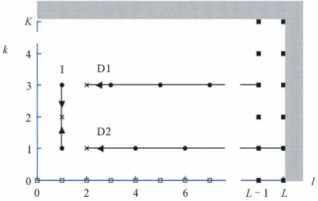
[image:5.595.59.287.499.643.2]Furthermore, it is instructive to consider the flow of information in Chebyshev space, associated with tempo- ral integration and spatial differentiation during iteration of Equation (13); see Figure 1. Note that for differentia- tion, only higher order modes contribute to the value of the Chebyshev coefficient at a specific modal point
Figure 1. Flow of information in Chebyshev space to a mo-dal point (k, l), associated with the coefficient aklm (the
mo-dal point is marked with a cross) from nearby modes when performing integration (I) in time as well as single differen-tiation (D1) or second differendifferen-tiation (D2) in space. Modes that are used for implementing initial conditions (empty squares) and boundary conditions (filled squares) are also indicated (two boundary conditions are shown).
whereas for integration, the Chebyshev coefficient at modal point k samples information from modal points both at k − 1 and k + 1. Modes that contribute to the val- ues of the integral or derivatives are marked. Modes out- side the computational domain (dashed region and be- yond) are defined to give zero contribution. The spatial domain behaviour is consistent with that the solution (13) is defined only to spatial orders less than BC. Thus L− LBC is the number of boundary conditions that should be imposed for all k and m.
L
In the diagram, modal points used for two boundary conditions are shown (filled squares). It is seen that any error occuring at high spatial mode numbers is amplified through the multiplicative terms in Equations (16), (17), and numerical instability could result. Since Chebyshev coefficients usually converge rapidly with mode numbers and since the boundary conditions are considered known, numerical stability is usually not compromised by this effect.
The initial condition is imposed at k = 0 for all modes with 0 ≤l < LBC≤ L and 0 ≤m≤ M and are marked by empty squares. The initial condition may be chosen arbi- trarily. If the initial condition requires many, or all, tem- poral modes for sufficient resolution, care must be taken not to conflict with the boundary conditions applied at high l values. Preferably, initial conditions are chosen so that they satisfy the boundary conditions.
Chebyshev Expansion of Boundary and Initial Conditions
The boundary conditions are implemented into the GWRM in the following way. We chose here to describe the case of Dirichlet boundary conditions; one at each end of a 1D spatial interval. Other types of boundary conditions may straightforwardly be implemented once this case is understood. For systems of equations with many boundary equations, subroutines for handling this are preferably programmed. The boundary conditions are Chebyshev expanded as
0
0 0
1
0 0
, ; ;
, ; ;
K M
km k m
k m
K M
km k m
k m
u t x p t p T T P
u t x p t p T T P
(18)We choose to apply discrete Chebyshev interpolation both for initial and boundary conditions since this pro- cedure has precisely the same effect as taking the partial sum of a Chebyshev series expansion and is easily com- puted [14]. We have generalized the well known one- dimensional Chebyshev polynomial interpolation of a function to three variables in time, physical space and parameter space, being shifted so that t
t t0,1 ,
0, 1
reduced in an obvious way to two variables for Cheby- shev expansion of the boundary and initial conditions discussed here, or further generalized to include more variables.
We thus approximate a function with the finite Chebyshev series
, ;
t x p
0 0 0
, ; K L M klm k l m k l m
t x p c T T T P
(19)with coefficients
1 1 1
1 1 1
2 2 2
1 1 1
, ;
klm
K L M
q r s k q l r m s
q r s
c
K L M
t x p T t T x T p
(20) where * * * , , π 1 cos , 1 2 π 1 cos , 1 2 π 1 cos 1 2q t q t r x r x
s p s p
q
r
s
t B t A x B x A
p B p A
t q K x r L p s M
The Chebyshev approximation given by Equations (19), (20) can be shown to be, under rather mild conditions, an accurate polynomial approximation of [14]. The boundary condition Chebyshev expansion coeffi- cients km
t x p, ;
and km are obtained by using the twodi- mensional version of Equations (19), (20) with the known functions
t p; and
t p; . Clearly, if
t p;
t p; 0 then all coefficients km and km
must be zero. From Equations (3) and (18) we obtain the relations
0 0 1 0 . Lkm klm l
l L
km klm l
l
a T x
a T x
(21)Since
x0 1 and
x1 1,(−1) = 1 to implement the two boundary conditions we use Tl(−1) = (−1)l
and Tl
at the highest modal numbers of the spatial Chebyshev coefficients;
, , , 1, 2 2 k L m km kmk L m km km
a S a S S
S (22)
for L being even (upper sign) or odd (lower sign), re-
0 L
l
(23) The Chebyshev coefficients in Equations (8) and (1 spectively, with L
2 2 01 ,l
klm klm
l
S a S a
lm b an ns3), for the initial condition exp sion, are computed by using the analytical form for u t x p
0, ;
in a two-di-mensional formulation of Equatio 20) in physic- cal and parameter space.
It should be noted that a useful simplification occurs fo
(19), ( r periodic boundary conditions, for which case
, ;0
, ;1
u t x p u t x p . This relation is only satisfied for ev omials. Considerable computation time is thus saved by only computing coefficients aklm
with even values of l.
In summary, initial and boundary conditions are i tia
en Chebyshev polyn
ni-
fully spec-
4) A basic and useful relationship is the identity TmTn = lly transformed into Chebyshev space by use of Equa- tions (19), (20) in suitable dimensional forms. All sub- sequent computations are performed in Chebyshev space, using Equations (13) and equations for the boundary con- ditions of the form (23). When sufficient accuracy in the coefficients aklm is obtained, the solution Equation (3)
is obtained in ysical variables. For periodic boundary conditions, coefficients aklm with l odd can be ne-
glected.
4. Nonlinearities in Spectral Space
ph
Nonlinear terms of the operator D are treated
trally in this method, in contrast to in pseudo-spectral schemes [13], where the nonlinearities are transformed to physical space, multiplied there and then transformed back to spectral space. This procedure causes the prob- lem of aliasing, which is avoided in the present scheme. In the GWRM, as nonlinear products are produced in spectral space, Chebyshev modes that lie outside the modal representation (K, L, M) will be truncated with associated loss of accuracy. As mentioned earlier it can be shown that truncated Chebyshev polynomials, because of their minimax properties, are the most accurate poly- nomial representation to this order [14].
For the sake of simplicity, we now discuss the han- dling of a second order nonlinearity in one-dimensional Chebyshev spectral space. Higher dimension cases are easily obtained from that of one dimension. We also omit the arguments of the Chebyshev functions, which are assumed identical.
Thus we wish to determine the coefficients ck in
0 m m 0 n n 0 k k
m n k
a T b T c T
M
N M N
(2
m n T|m n|
2 , which “linearizes” expressionscon-oducts of Chebyshev polynomials. Since all variable expansions have the same number of modes within the same space (temporal, physical or parameter
T
space), we may assume that NM in Equation (24). After some algebra, the following exact expression is determined:
1 2 M 1 k kc f
0 0
1
m k k m
m
a b
(25)being valid for 0 ≤ k ≤ 2M
km
b|k m|
. Here fk 1 2 for k0,
and for . Th summ
dex o
1
k
f
ld rend
0 k
ultipl
e prime on the in
ation sign d of b
denotes that all occurences of a zero f a an shou er a m ying factor of 1 2. Note that only the coefficients for the employed spectral space are computed (we thus compute ck for 0 ≤ M); other
terms are truncated. The computation is best facilitated by creating a procedure that ca e repeatedly called also when computing coefficients for higher order nonlineari- ties.
5. So
k ≤
lution of Algebraic
s of
nts
ound
wh ) are
im
n b
System
Equations for Chebyshev Coefficie
The GWRM solution to an initial-value problem is f en the Chebyshev coefficients of Equation (13 determined to sufficient accuracy. For a linear problem, the coefficients can be obtained by a simple Gaussian elimination procedure. Nonlinear differential equations, however, lead to nonlinear algebraic equations and these may be difficult to solve numerically [15]. We thus need a robust nonlinear solver that converges both globally and rapidly. Although various such methods already exist [15], we have found it rewarding to develop a new semi-implicit root solver, SIR [16], as described below.
The GWRM is well adapted for solution using itera- tive methods for two reasons. First, Equation (13) can be
mediately cast in the fixed-point iterative form
x x (26) where the solution vector xh
coefficients to be determ d the vector func- ere
ined, an
contains the Chebyshev
qrs
tion
a
reflects the functional forms of Aqrs and Fqrs.
Second, all iterative methods require an initial estimate of the olution vector, and if this deviates much fr the solution to be determined, numerical instability re- sults. For the GWRM, the coefficients that correspond to the solution for the entire time domain (the roots of the equations) may deviate strongly from the coefficients of the initial state. One of the simplest and most frequently used solvers, Newton’s method, features a fairly limited domain of convergence [15,17,18], however. Because the initial guess in the case of the GWRM is precisely the initial condition, there always remains the possibility to reduce the solution time interval
s too om
0,1
t t , for example by using subdomains as described below, so that the solu- tion Chebyshev coefficients becom fficiently close to the initial Chebyshev coefficients. This, incidentally,
shows that a GWRM formulation of a well posed initial- value problem in principle always will lead to a solution, although we do not prove this rigorously at present.
Newton’s method is usually globally improved by the addition of line-search methods, in which the itera
e su
tion st
ulation. Instead of direct iteration, us
A (27) or, in matrix form
ep size is decided from the minima of the function, the roots of which are to be determined. Unfortunately, these methods may land on spurious solutions, corresponding to local minima rather than to true zeroes of the function. We have thus developed the semi-implicit root solver (SIR), being an iterative method for globally convergent solution of nonlinear equations and systems of nonlinear equations. By “global” is here meant that correct global solutions are usually (but not always) found, having the the new feature that they are never local, non-zero min- ima. It is shown in [16] using a set of test problems, that global convergence is at least as good as for Newton-like line-search methods. Convergence is quasi-monotonous and approaches second order in the proximity of the real roots. The algorithm is related to semi-implicit methods, earlier being applied to partial differential equations. We have shown that the Newton-Raphson and Newton methods are limiting cases of the method. This relation- ship enables efficient solution of the Jacobian matrix equations at each iteration. The degrees of freedom in- troduced by the semi-implicit parameters are used to control convergence.
Details of SIR are given in [16]; we here only briefly describe the basic form
ing Equation (26), the semi-implicit method leads in- stead to the problem of finding the roots to the N equa- tions
N
m
x
1
;
mn n n m m
n x
x x x
x
x
x A;
x A x (28)
The system (28) has the same solutions as t system, but contains free parameters in the fo co
he original rm of the mponents mn of the matrix A. These parameters are determined by specifying the values of m xn, the gradients of persurfaces m. The latter gradients control global, quasi-monotonous and su con- vergence. In SIR,
the hy
perlinear
0
m xn
for all m≠ n, whereas
m xm
is finite and is chosen to produce limited step lengths and quasi- convergence; it usually
s zero after some initial iterations. Since New- ton’s method is a limiting case of the present method, namely when all
monotonou approache
s
0
m xn
, rapid second order con- vergence is generally approached after some iteration steps. The relation ton’s method fortunately leads to approximately similar numerical work, essen- tially that of solving a Jacobian matrix equation at each
iteration step.
There are two aspects of the GWRM that are of par- ticular importance for the root solver. First, the algebraic equations to be solved are polynomials of the same order as the nonlinearity of the original differential equations. For example, second order nonlinear pde’s lead to the solution of a system of second order polynomial equa- tions by SIR. Since a large class of problems in physics, formulated as pde’s, feature second (or third) order nonlinearities, there is a potential to device more efficient versions of SIR where this fact has been utilized. Second, most of the computational time in SIR, when applied to the GWRM, is not spent on matrix equation solution, but rather on function evaluation. If the functions n are
formulated and evaluated more economically, computa- tional efficency may be improved.
We conclude this section by stating that the SIR algo- rithm has turned out to be robust and well suited for all G
patial Subdomains
atrix in- he num- WRM applications tried to date. Further development would focus on the possibility to enhance SIR efficiency by economizing the handling and evaluation of the poly- nomial Equation (13).
6. Temporal and S
The number of arithmetical operations due to m version typically feature a cubic dependence on t
ber of unknowns. The root solver, applied to Equation (13), thus may dominate computational time. Applied to Equation (3), straightforward application of GWRM and SIR would require about
K1
3 L1
3 M1
3operations for each iteration when solving Equation (13). Using LU decomposition rath
number of operations is reduced to
er than matrix inversion, the
3
[15]. As shown in the examples of the next section, this may often be an acceptable amount of work.
In more complex calculations, efficiency requires the temporal and spatial domains to be separated into subdo- mains. This enables a linear rather than a cubic depend- ence of efficiency on, for example, the number of spa-tial modes applied to the entire domain, given that the number of subdomains is proportional to L. Assume that the temporal and spatial domains are divided into Nt and
Nx subdomains, respectively. This reduces 3 opera-tions to
3 3
t
N N 3
2
1 1 1 3
3
x t x
t x
K N L N M
N N
operations when solving a particular problem, assu ing that the same total number of modes are sufficient in both
m cases. As an example, for K = L = 11, M = 2 and Nt = Nx = 3there would be a reduction from about 2.7 × 10⁷ to 3.3 ×
105 operations Additionally it should be noted that the
functions m in SIR will become substantially less com-
plex when subdomains are used, with resulting reduced computational effort.
Temporal and spatial subdomains must be implemented differently. For the temporal domain the procedure can be m
only kn
of piece-wise so
ore straightforward. As initial condition for each do- main, we here simply use the end state of the previous one. It should be recalled, however, that a GWRM (as well as any WRM) solution is not per se a Chebyshev approxi- mation of the true solution, but rather stems from a mini- mization of the residual, including information concern- ing the differential formulation of the problem, over the solution domain. Simple averaging (by using a few modes) over regions with strong temporal gradients is thus likely to produce large errors, due to the poorly approximated differential character of the problem. As will be shown, a preferred solution is to use an adaptive scheme, which uses few modes by default in each subdomain, but in- creases this number whenever accuracy so requires. Fur- thermore, the use of temporal subdomains is beneficial for SIR convergence, since the initial condition for each do- main will be closer to the final solution than what would be the case using a single temporal domain instead.
Spatial subdomains must be treated in another fashion. The reason is that boundary conditions are usually
own at the exterior, rather than at interior, boundaries. A computation is not conveniently progressed success- sively through a sequence of spatial subdomains, as for temporal subdomains. Instead the boundary conditions are imposed on the outermost spatial subdomains, and the subdomains are connected at interior boundaries through continuity conditions. The functions themselves and their first derivatives are continuous across each subdomain (interior) boundary. All spatial subdomains are updated in parallel at each solution iteration. Computationally, the choice of procedure is a nontrivial task. Due to the large coefficients, appearing in higher order derivatives (see Equations (16), (17)), derivative matching is sensitive to small errors and numerical instability may result. Instead we have found that a ”handshaking procedure” where the functions are allowed to overlap into neighbouring do- mains, and are doubly connected, yields improved stabi- lity over derivative matching.
Subdomains may also be introduced into the physical parameter domain, if desired. The final set
applications will be published separately.
7. Example Applications of the GWRM
y and ed by
ary differential equations is first so
structure near th
wave equations without and with a fo
earized systems of ideal and resis-tiv
he Match Equation
idly until the nsumes is balanced by the oxygen that We now turn to the important questions of accurac efficiency. In this section, the GWRM is compar example to other methods for solving partial differential equations, that use time discretization in the form of fi- nite differencing. Even though the GWRM generates semi-analytic solutions, it must be comparable to these standard methods with regards to accuracy and efficiency to be of practical use.
To study performance when applied to nonlinear problems, a stiff ordin
lved. Adaptive, temporal subdomains are here showed to provide high accuracy and efficiency.
As a second example the nonlinear, 1D viscous Burger equation is solved. It features a shock-like
e boundary. It is shown that GWRM accuracy is com- parable to that of the (explicit) Lax-Wendroff and (im- plicit) Crank-Nicolson schemes for a similar number of floating operations.
Next we study a problem with two strongly separated time scales. For the
rcing term, the GWRM turns out to be considerably more efficient than both the Lax-Wendroff and the Crank- Nicolson solution methods when tracing the dynamics of the slower time scale.
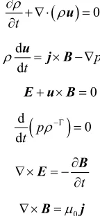
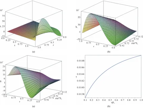
The GWRM is finally applied to the demanding prob-lems of solving the lin
e magnetohydrodynamic (MHD) equations. Similar problems are of key importance when studying the sta-bility of magnetically confined plasmas for purposes of controlled thermonuclear fusion.
7.1. Introductory Example: T
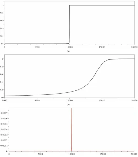
When a match is lighted, the flame grows rap oxygen it co
comes through the surface of the ball of flame. A simple model for the flame propagation in terms of the ball ra- dius u t
is2 3
d du t u u (29) with
0 , 0 2u t . (30) For small values of this prob
stiff through the presen of a ramp
lem becomes very at
ce t1, repre- se
is pro
nting the explosive g wth of the ball towards its steady state size [19]. We have solved th blem by using Equation (25), transforming it to the form of Equa- tion (2), yielding a set of equations corresponding to Equation (13) in which spatial and parameter modes are
omitted. A solution with 0.0001
ro
is presented in
Figure 2. We have imposed an accuracy of = 1.0 × 10⁻⁴. The GWRM solution d with the exact
solution to Equations (29), (30);
is compare
1 a t 1
u t W ae
(31)
1 1
a
where and W
Clearly, for this sm
is the Lambert all value of
W function.
el
the is very and hard
di
ramp
distinct to resolve. Consequently, explicit finite fference methods will need extrem y small time steps to resolve this problem. An optimised Matlab solution to the problem uses implicit methods that may reduce the computational effort to about 100 time steps, taking a few seconds on a tabletop computer. The GWRM solu- tion in Figure 2 uses 69 temporal domains and takes just about the same amount of computational time, but has the additional feature to provide analytical approxima- tions to the solution in each domain. These may be of particular interest in the ramp region. For efficiency, the temporal domain length has been automatically adapted as follows. Since T tn
1, we obtain the criterion foraccuracy
aK1aK
a0 a1
.In performing the computation, a default of 10 time s is assumed and K = 6 is d th hout. If th
is in the transformation from the pla- te
subdomain use roug
e accuracy criterion is satisfied, the subdomain length is doubled at the next domain, and if not it is halved. In the latter case, the calculation is repeated for the same subdomain until the accuracy criterion is satisfied. This goes on as the calculation proceeds in time until near the endpoint, where the subdomain length is adjusted to land exactly on the predefined upper time limit. Due to the stiffness of the problem in Figure 2, the subdomains are concentrated near t = 1.0 × 10⁴ where the subdomain
length may be as small as about 2 time units. The auto- matic extension of the subdomain length in smoother regions saves considerable computational time; at the end of the calculation the subdomain length is several thou- sand time units.
The essential information provided by the computa- tions of Figure 2
au u = 0 to the plateau u = 1 at t = 1.0 × 10⁴. Perhaps
(a)
(b)
(c)
Figure 2. (a) Solution to the match equation (29), with δ = 0.0 K = 6, ε= 0.0001, using initial subdomain length of (2/δ)/10;
with the solutions at lower and higher times t. This is an
tion, high efficiency is also obtained, comparing well with highly optimised
001,
(b) As (a), with ramp region at t = 1/δ enlarged; (c) Absolute error for the computation of (a).
Equation (29) there are quadratic as well as cubic interesting topic for future studies. in
nonlinearities. As a result a global, low mode approxima- tion of the solution is not trivially obtainable. The transi- tion region needs a certain amount of resolution to “tie”
[image:10.595.61.540.84.631.2]M
e on. The one- uation
atlab routines for implicit finite difference methods.
7.2. Accuracy; Burger’s Equation
Burger’s equation is of particular interest since it is nonlinear and contains two time scales as a result of th competition between convection and diffusi
dimensional Burger partial differential eq
2
2
u u u
u
t x x
(32)
Thus contains essential physics, such as convective nonlinearities and dissipation, expected to be encoun- tered also in more complex problem
and MHD. Here
s of fluid mechanics
denotes (kinematic) viscosity. Since th
ti
f transformation [6]
is equation has an analytical solution, it provides ex- cellent benchmarking.
7.2.1. Exact Solu on of Burger’s Equation
The exact solution to Equation (32) is found by first in- troducing the Cole-Hop
2
u
x
to produce a standard diffusion equation in
(33)
t x, and then by using the Fourier method. The result, for the boundary conditions
, 0
u t u t,1
0 is
2 2π
0
2π sin π
,
π
m t m m
mA e m x
u t x
x
2 2π (34)0
cos
m t m m
A e m
with coefficients
1
0
2 cos π d
m
A
x m x x, (35) where
x
0,x . As an example, the initial condi-tion
0,
1
u x x x in
(36) results
3x2 2x3
12 x e
. (37) It shoul
Equation (
d be noted that the sums of the exact solution 34) may need to be carried out over a large number of terms for sufficient accura
poor convergence at low viscosity.
cy, because of the As 0.005 at le
functions
radients are often difficult to resolve in spectral re
condition
ast 100 terms are required to compute a solution that gives a reasonably accurate solution near t = 0. Further- more, in contrast to polynomials or Chebyshev polyno- mials, the exponential and trigonometrical of Equation (34) are costly to evaluate numerically. This is one example of an exact solution that is of limited prac- tical use.
The most challenging aspect of the Burger equation, from the modelling point of view, is the shock-like structure that evolves for weak dissipation. The as- sociated g
presentations. Highly accurate modelling may require a high number of Chebyshev modes. The case we study develops a strong gradient near the boundary x = 1, and is representative of the gradients in, for example, edge pressure or temperature, encountered in magnetohydro- dynamic computations in fusion plasma physics model- ling. The structure may also appear when modelling lo- calized resistive instabilities in tokamak and reversed- field pinch magnetic fusion configurations. It is desired that the GWRM should be able to resolve these structures for limited values of mode numbers. To see the dif- ference as compared to standard modelling, we make comparisons to solutions obtained from the standard explicit Lax-Wendroff and implicit Crank-Nicolson finite difference schemes for partial differential equations [15].
7.2.2. GWRM Solution of Burger’s Equation
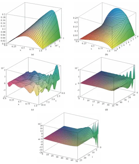
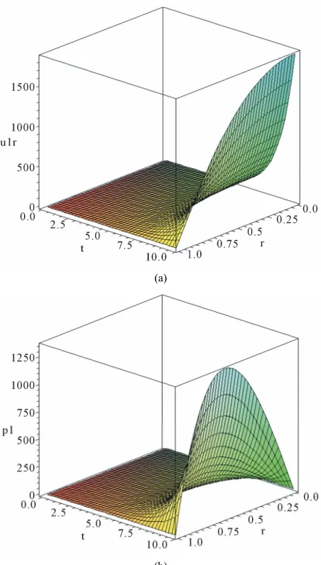
In Figure 3(a), the GWRM solution of Burger’s equation for boundary conditions u t
,0 u t
,1 0 and initial
x x
1 x
iven by
is shown. Nine te he solution is vali
mporal (K
(viscos- = 8), eleven spatial (L = 10) and three parameter
ity) modes (M = 2) were required to obtain an error better than 1% after 7 iterations. T d within the domains g
t0,t1 0,5 ,
x x0, 1
0,1 and
0, 1
0.01,0.05
, and is displayed for fixed t = 2.5.Note that the solution was attained for all viscosities in the given range in a single computation. It is seen that a sharp gradient builds d pro- ues of viscosity. If the number of temporal or spatial modes are reduced somewhat, the same accuracy is retained everywhere except for near the edge x = 1. Since the “exact” Cole-Hopf solution con- verges slowly at these low values of
up r small val
near the e ge, being most found fo
, the obtained GWRM semi-analytical solution is actually computa- tionally more economical to use in applications.
To enable comparisons with explicit and implicit finite difference partial differential equation solvers, we will now fix viscosity to 0.01 and compute the solutions as functions of t and x. The Burger equation, defined as ab
atter tw
odes. With mode nu
ove but now using t1 = 10, is solved using all GWRM,
explicit Lax-Wendroff, and implicit Crank-Nicolson methods [15]. The l o schemes are accurate to second order in both time and space.
For the GWRM solution, two spatial subdomains with internal boundary at x = 0.75 are used. A similar result would be obtained using only one spatial domain with slightly higher number of spatial m
dis-played in Figures 3(b) and (c). The peak near t = 0 in
Figure 3(c) is due to the poor convergence of the exact solution of which 60 terms are used.
7.2.3. Lax-Wendroff Explicit Finite Difference Solution of Burger’s Equation
We now turn to solution of the Burger equation using finite difference methods. Accurate solutions are not edge
gradie p length required
straightforwardly obtained because of the strong nt. Let us estimate the spatial ste
for a global error = 0.001. A second order estimate of the mid-point error resulting from finite spatial differ- encing with spacing x is
1 1
2
2 2
1 2
8
f x x f x x f x
f x
(38)
x
where a prime denotes spatial differentiation. F exact solution it is found that
rom the
max f x = 20
= (2.05, 0.94). A maximum global error of δ = 0.001 thus requires
.3 at (t, x)
x
< 0.02.
and becaus
ma becomes limited, however. A
The Lax-Wendroff finite difference scheme is widely used because of its reliability e it is accurate to second order in both time and space. Since it is ex- plicit, the ximum time step
von Neumann analysis of the Lax-Wendroff method applied to the Burger equation (32) features the limiting cases of strong convection or strong diffusion. When convection dominates the CFL condition t x uc ,
where uc is a characteristic fluid velocity, results. This
condition characterises the required causality on the so- lution grid for hyperbolic problems. When the diffusion term dominates, the problem is parabolic an e step is ited to
d the tim lim t x 2 2
t crit by causality. Computations show that the latter criterion is the more relevant one for the present Burger problem.Recall that accuracy requires x< 0.02 according to Equatiom (38). Th ment with the value
is is in reasonable agree
x
≤ 1/70, that was found numerically. For
0.98
t t
crit, the number of time steps
00 for the given accuracy. Th rror of a Lax-Wen- droff computation is shown in Figure 3(d). High accu-racy is obtained everywhere except near the maximum
Using Maple 12 on the same platform for both methods, the Lax-Wendroff method needs 50% less time than the GWRM. It is thus somewhat more ac-curate for the same number of computational operations in this case. Note, however, that the discussion in Section 3.1 shows that for the case of a single spatial domain, the boundary conditions would be periodical (or homogene-ous) in which case odd spatial mode numbers can be omitted and an eight-fold gain in efficiency would be
attainable. The GWRM solution has also the advantage of being in analytic form whereas the Lax-Wendroff so-lution is purely numeric.
7.2.4. Crank-Nicolson Implicit Finite Difference Solution of Burger’s Equation
Next, we solve the Burger
becomes
spatial gradient.
equation using the Crank- Nicolson method. This scheme allows for arbitrarily the
functi t the previous and
10 e e
large time steps by using an implicit approach where onal values are determined both a
present time steps. On the spatial scale, the resolution
x
≤ 1/70 is, however, still needed to obtain a global accuracy of 0.001. To avoid costly matrix inversion at each time step, due to the implicit finite difference for- mulation, a tridiagonal matrix solution procedure has
n developed [15] that radically speeds up the calcula- tions for linear equations. To be able to use this scheme for the nonlinear Burger equation, we advanced the lin- ear diffusive term using the standard Crank-Nicolson method, but advanced the nonlinear convective term ex- plicitly. As a result, a von Neumann analysis shows that the time step is no longer unrestricted, but must obey the relation
bee
2
2 c
t u
. Note that this relation is inde- pendent of x.
For a time step t = 1/500 and with x = 1/70, an accuracy of 0.001 was achieved for the Burger equation, as shown 3(e). The computer time used was about half t of
in Figure
hat the Lax-Wendroff method. For general
no ord
quation is more economic than the “exact” Cole-Hopf solution for use in applications at low nlinear problems, when a linear higher er term that can be advanced explicitly does not exist, this method may be less accurate however. The reason is that, for making use of efficient tridiagonal matrix solving, the differential equation should be time linearized, which introduces errors.
7.2.5. Conclusions on Solution of Burger’s Equation
Interestingly, we have found that the analytical GWRM solution of Burger’s e
(a) (b)
(c) (d)
(e)
[image:13.595.56.539.80.650.2]
periodic boundary conditions. The GWRM has the addi- tional advantage of providing approximate, analytic solu- tions.
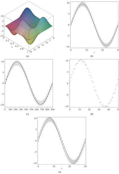
7.3. Efficiency: The Forced Wave Equation
Problems in physics often feature multiple time scales, dyna- whereas it may be of main interest to follow the moics of the slowest time scale. Efficient partial differ-ential equation solvers therefore must be able to employ long time steps, retaining stability and sufficient accu-racy. By omitting resolution of the finer time scales, im-proved efficiency and the possibility to study complex systems are expected. As a test problem, we choose a wave equation with a forcing (source) term, also called the inhomogeneous wave equation:
2 2
2 2 ,
u u
f t x
t x
with boundary and initial conditions
(39)
, 0
,1 0u t u t
0, sin
πu x n x
0, sin
u
x A x
t
Here A, n,, and
inare free parameters, and
,
2 2
sin s
f t x A t x
function. The exact solution is
is the forcing
, cos
π 0.5
sin
π
sin
u t x n t n x A t
sin x (40)for mπ, with m an integer. This problem has the stem and forcing function time scales
separate sy 2
n and 2π. Using the parameter value 1, A10,
π15
, 3π and n3, the ratio of these time scales becomes R
nπ
1 45. Thus he g(40) here in uced a time scale much t forcin term in has trod
f the “unperturbed” s
GWRM, longer than that o ystem.
7.3.1. GWRM Solution of the Forced Wave Equation
We now wish to solve Equation (39) using all
Lax-Wendroff and Crank-Nicolson methods. The prob-lem is thus posed as a set of two first order partial dif- ferential equations:
2
,
U u
2 f t x
t
x
u U t
(41)
with boundary and initial conditions corresponding to those of Equation (39). The GWRM solution, using one
condition, which for this
spatial domain with K = 6 and L = 8, is rapidly obtained within a single iteration with a tolerance of 1.0 × 10⁻⁶ for
(system) time scale and follows the slower (forced) time scale in an averaging sense. This is shown in more detail in Figure 4(b), where the temporal evolutions of both the exact and the GWRM solutions are shown jointly for fixed x. The averaging character of the solution remains at least for all values K≤ 20.
7.3.2. Lax-Wendroff Explicit Finite Difference Solution of the Forced Wave Equation
We now turn to finite difference solution of Equation (39) using the Lax-Wendroff method. Being an explicit method, it must obey the CFL
the coefficient values. It is displayed in Figure 4(a). The solution behaves as desired; it averages over the faster
case becomes t x. We find that sufficient acc is obtained for
uracy
x
≤ 1/30. Thus the maximum allowed time step is 1/30, and the number of time steps becomes 900 for the domain
t t0,1 0,30
. The calculation re-quires about ten times more computer time than the GWRM. It can be seen in Figure 4(c) that the solution initially traces t exact solution, but thereafter follows the slower time scale. The solution appears not to aver- age as accurately as the GWR ov r the fast time scale.
7.3.3. Crank-Nicolson Implicit Finite Difference Solution of the Forced Wave Equation
The Crank-Nicolson method, being implicit, has no time step restriction and no amplitude dissipation and would perhaps intuitively be well suited for the present problem
he
M e
. qua- [6] Additionally, to avoid time-consuming large matrix e tions, the so-called Generalized Thomas algorithm uses a block-tridiagonal matrix algorithm that substan- tially speeds up the calculations at each time step. If the associated sub-matrix equations are solved for, rather than computing inverse matrices, a gain from Gauss elimination O((MN)3/3) operations to O(5M3N/3) opera-
tions is possible, that is the speed gain factor becomes
N2/5. Here the number of equations M = 2 and the num-
ber of spatial nodes N = 30. The handling of a number of sub-matrix equations, required at each time step, is still limiting performance however. With x = 1/30, tem- poral resolution requires at least 50 time steps. Using matrix inversion, the corresponding computation is about three times slower than Lax-Wendroff and thus about 30 times slower than that of the GWRM. A speed gain of a factor three is expected by solving the sub-matrix equa-tions rather than determining inverse matrices, but the GWRM remains considerable faster. It should be noted that the sub-matrices used in the Thomas algorithm are here only 2 × 2 in size. Thus negligible time is spent in matrix inversion; it is rather the extensive use of matrix manipulations in the algorithm that affects efficiency. The solution is shown in Figure 4(d) and in Figure 4(e)
(a) (b)
(c) (d)
(e)
[image:15.595.96.498.84.670.2]