Simulation and Modelling of Smart Beams with Robust
Control Subjected to Wind Induced Vibration
Amalia Moutsopoulou1, Georgios Stavroulakis2, Tasos Pouliezos2 1Department of Civil Engineering, Technological Educational Institute of Crete, Crete, Greece 2Department of Production Engineering and Management, Technical University of Crete, Crete, Greece
Email: [email protected], [email protected], [email protected]
Received May 22, 2012; revised June 28, 2012; accepted July 9,2012
ABSTRACT
This paper presents some recent developments in modelling and numerical analysis of piezoelectric systems and con-trolled smart structures based on a finite element formulation with embedded control. The control aims at vibration sup-pression of the structure subjected to external disturbances, like wind and noise, under the presence of model inaccura-cies, using the available measurements and controls. A smart structure under dynamic loads is analysed and comparison between results for beam with and without control is made. The numerical results show that the control strategy is very effective and suppresses the vibrations of the structure.
Keywords: Smart Structures; Finite Element Formulation; Uncertainty; Robust Performance; Reduced Order Control
1. Introduction
The intelligent material sector has broadly motivated research interest during the last decades. Materials are classified as intelligent if they exhibit the ability to sense a certain stimulus and initiate a reaction to it in a con-trolled manner [1-11]. An intelligent structure is a struc-tural system or member with embedded sensors and ac-tuators, combined with a control system that automates the structure's reaction to external loadings acting on it, by attenuating their influence or improving desirable responses. Development in this scientific discipline is aided by advances in material science as well as in the field of control. Material science research has spurred the development of new materials that can be incorporated in structures to be used as actuators and sensors [9-11].
In this paper, we address the problem of vibrations of intelligent structures. Stimuli may come from external perturbations of the system, disturbances or excitation that may cause structural vibrations, such as wind load-ing or earthquakes. An intelligent structure is expected to be able to sense the vibration and counteract it in a con-trolled fashion, so that vibration of the system be reduced and contained. To that end, a number of intelligent mate-rials may be used as actuators and sensors. [9-11] Piezo-electric materials, memory materials, electrostrictive and magnetostrictive materials are such materials. In this work, we focus on the use of piezoelectric materials, given that they exhibit good sensing and actuation properties.
Among the commonly used optimal control schemes
are LQR, and H. It is known that if the controller is not robust enough, the uncertainties of the system may destroy the efficiency of the controller. The H, control provides better robustness than LQR [12-14]. The aim of this work is to design an H, robust controller for a beam bonded with piezoelectric sensors and actuators and to investigate the behaviour of the controlled beam. First, a detailed shear-deformable (Timoshenko) model for a laminated beam structure is developed. A finite element formulation is presented for the model. Quad-ratic Hermitian polynomials are used for the transverse and rotational displacements, respectively. The differen-tial equations are based on the Timoshenko beam theory [15]. The governing state equation is established and used for the design of the control. The numerical simula-tions carried out on the laminated beam shows that the vibration of the system is significantly suppressed within the permitted actuator voltages. Herein the integration of control into a home-made finite element code developed in MATLAB is presented [16]. The numerical solution of the H feedback controller has been done by using a nonconvex, non differentiable optimization approach with the usage of HIFOO software within MATLAB [14,17]. For the numerical results wind type loads are taken into account. The effectiveness of the technique in the model-ling of the standard uncertainties is also presented.
2. Mathematical Modelling
tions is considered. Four pairs of piezoelectric patches are embedded symmetrically at the top and the bottom surfaces of the beam, as shown in Figure 1. The beam is made from graphite-epoxy T300-976 and the piezoelec-tric patches are PZT G1195N. The top patches act like sensors and the bottom like actuators. The resulting composite beam is modelled by means of the classical laminated technical theory of bending. Let us assume that the mechanical properties of both the piezoelectric mate-rial and the host beam are independent in time. The thermal effects are considered to be negligible as well [5, 6].
The beam has length L, width W and thickness h. The sensors and the actuators have width bS and bA and
thickness hS and hA, respectively. The electromechanical
parameters of the beam are given in the Table 1.
2.1. Reduced Piezoelectric Equations
In order to derive the basic equations for piezoelectric sensors and actuators (S/As), we assume that:
[image:2.595.58.289.367.498.2] The piezoelectric S/A are bonded perfectly on the host beam;
Figure 1. Beam with piezoelectric sensors/actuators. Table 1. Parameters of the composite beam.
Parameters Values
Beam length, L 0.3 m
Beam width, W 0.04 m
Beam thickness, h 0.0096 m
Beam density, ρ 1600 kg/m3
Young’s modulus of the beam, E 1.5 × 10¹¹ N/m2
Piezoelectric constant, d31 254 × 10−12 m/V
Electric constant, ξ33 11.5 × 10⁻³ V m/N
Young’s modulus of the piezoelectric element 1.5 × 10¹¹ N/m2
Width of the piezoelectric element bS = ba = 0.04 m
Thickness of the piezoelectric element hS = ha = 0.0002 m
The piezoelectric layers are much thinner then the host beam;
The piezoelectric material is homogeneous, trans-versely isotropic and linearly elastic;
The piezoelectric S/A are transversely polarized (in the z-direction) [5].
Under these assumptions the three-dimensional linear constitutive equations are given by [4],
11 31
55 0
0 0
xx xx
z
xz xz
Q d
E Q
11 31
(1)
z xx xx z
D Q d E (2) where xx, xz denote the axial and shear stress com-
ponents, Dz, denotes the transverse electrical displace-
ment; xx and xz are a axial and shear strain compo-
nents; Q11, and Q55, denote elastic constants; d31, and ξ33,
denote piezoelectric and dielectric constants, respectively. Equation (1) describes the inverse piezoelectric effect and Equation (2) describes the direct piezoelectric effect.
Ez, is the transverse component of the electric field that is
assumed to be constant for the piezoelectric layers and its components in xy-plain are supposed to vanish. If no electric field is applied in the sensor layer, the direct pie-zoelectric Equation (2) gets the form,
11 31
z xx
D Q d (3) and it is used to calculate the output charge created by the strains in the beam [3].
2.2. Equations of Motion
The length, width and thickness of the host beam are denoted by L, b and h, respectively. The thickness of the sensor and actuator is denoted by hs and ha. We assume
that:
The beam centroidal and elastic axis coincides with the x-coordinate axis so that no bending-torsion cou-pling appears;
The axial vibration of the host beam centreline is considered negligible;
The displacement field {u} = (ux, uy, uz) is obtained based on the usual Timoshenko assumptions,
, , ,
, , 0
, , ,
ux x y z z x t uy x y z
uz x y z x t
(4)
where φ is the rotation of the beams cross-section about the positive y-axis and w is the transverse displacement of a point of the centroidal axis (y = z = 0).
The strain displacement relations can be applied to Equation (4) to give,
xx z xx z
x x
(5)
[image:2.595.60.284.542.732.2]We suppose that the transverse shear deformation is equal to zero [2]. In order to derive the equations of the motion of the beam we use Hamilton’s principle,
1 2
t
t
UW
dt0 (6) where T [6] is the total kinetic energy of the system, U is the potential (strain) energy and W is the virtual work done by the external mechanical and electrical loads and moments. The first variation of the kinetic energy is given by, 2 0 2 1 d 2 2 s A r V h h L h h u u T V t t b z t t
d dz xt t (7)
The first variation of the kinetic energy is given by,
2 11 0 2 1 d 2 2 s A V h h L h h U V b Q z
z d dz xx x
(8)
If the load consists only of moments induced by pie- zoelectric actuators and since the structure has no bend- ing twisting couple then the first variation of the work has the form [6],
0
L
W b
MA dx x
(9)
where MA is the moment per unit length induced by the
actuator layer and is given by,
2 2 11 31 2 2 d d A A h h A
h h xx h h z
M z z zQ
Ad A Az A
V E z E
h
(10)
2.3. Finite Element Formulation
We consider a beam element of length Le, which has two
mechanical degrees of freedom at each node: one transla-tional ω1 (respectively ω2) in direction z and one
rota-tional φ1 (respectively φ2), as it is shown in Figure 2.
The vector of nodal displacements and rotations qe is
defined as [3],
1, ,1 2, 2
re
[image:3.595.60.287.611.723.2]q (11)
Figure 2. Beam finite element.
The beam e (x, t) and the
be
lement transverse deflection ω
am element rotation ψ(x, t) of the beam are continuous and they are interpolated within by Hermitian linear shape functions Hi and Hias follows [4],
4
1 4 1 , , i i i i i ix t H x q t
x t H x q t
(12)This classical finite element procedure leads to the ap-proximate (discretized) variation problem. For a finite element the discrete differential equations are obtained by substituting the discretized expressions 12 into Equa-tions (7) and (8) to evaluate the kinetic and strain energies. Integrating over spatial domains and using the Hamiltons principle 6 the equation of motion for a beam element are expressed in terms of nodal variable q as follows,
m
e
Mq t Dq t Kq t f t f t (13) where M is the generalized mass matrix, D the visc
on ous damping matrix, K the generalized stiffness matrix, fm
the external loading vector and fe the generalized c -trol force vector produced by electromechanical coupling effects. The independent variable q(t) is composed of transversal deflections 1 and rotations 1, i.e., [7]
1
1n n q t
(14)
where n is the number of nodes used in analysis. Vectors
ω and fm are positive upwards. To transform to state-
space co rol representation, let (in the usual manner),
q t nt
x t q t (15)
Furthermore to express f te
as Bu t
we write itas *
e
f u where *
e
f the piezoelectric is for a unit app on the co esponding actuator, and u represents the voltages on the actuators. Furthermore,
force
lied rr
m
d t f t is the disturbance vector [18]. Then,
2 2 2 21 1
2 2 2 2
1 * 1
n n n n
n n n n
e
O I
x t x t M K M D
O O
u t
M f M
(16)
Ax t Bu t Gd t u t
The previous description of the dynamical system will be augmented with the output equation (some d
ments or velocities are measured) [4],
T
isplace-
1
3
n1y t x t x t x t Cx t (18)
3. Statemen
ith known elastic, piezo-electric and viscous properties. A more realistic question
In this formulation u is n × 1 (at most, but can be smaller), while d is 2n × 1. The units used are compatible for instance m, rad, sec and N.
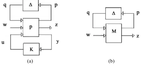
[image:4.595.310.535.87.197.2](a) (b)
Figure 3. Uncertainty modelling.
satisfies
t of the Robust Control Problem
The optimal control problem is initially studied for the
nominal system, i.e., the beam w 1. Since controller K is known. Figure
3(a) can be simplified to Figure 3(b). Given this struc ture it is kn
1) The sy
concerning the robustness of the control in the presence of defects is also addressed. The fact that the system is in subjected to disturbances, such as the wind power, as well as the noise of measurements, is taken into account. The mathematical pattern being used in the design is an ap-proximation of the real one. Further, two control laws for the composite beam are designed in order to suppress the vibrations. Because of its linearity and easy implementa-tion, the linear quadratic regulator (LQR) [13] is pre-sented first. The response of the controlled nominal and damaged beams is investigated. In order to take into ac-count the incompleteness of the information about the eventual damages and external additional influences a robust H controller is designed [12,14]. A system
analysis is made on condition that the system is not accu-rate but includes uncertainty that may be related to some kind of damage [7].
For practical applications both algorithms need several trial-and-error design iterations in order to provide appro-priate control voltages, since the piezoelectric actuators can be depolled by high oscillating voltages. The effec-tiveness of the proposed control strategies is investigated with the help of numerical simulations [3].
3.1. Robustness Analysis
The following three steps are taken in the robustness analysis [13,14,19]:
1) Expression of an uncertainty set by a
mathemati-an
cal model.
2) Robust stability (RS): check if the system remains stable for all plants within the uncertainty set.
3) Robust performance (RP): if the system is robus-tly stable, check whether performance specifications are met for all plants within the uncertainty set.
To perform the robustness analysis, the interconnec-tion of Figures 3(a), (b) will be used.
Δ define the uncertainty, Μ define the nominal sys-tem, w are the inputs (the mechanical force and the noise of the system), z are the outputs (the state vector
d the control vector). The uncertainty included in Δ
-own that [16,19],
stem (M, Δ) is robustly stable if,
11
ˆpn 1
I
j
(19) where,
su
1
ˆ ,detinfI M 0
(20) is the structure singular value of M given the
struc-certainty set
tured un .
2) The system (M, Δ) exhibits robust pe
rformance if,
sup j 1
0
ˆn
I
where,
(21)
0
and has the same structure as Δ but dimensions
nding to (w,z). Unfortunately, only bounds on
μ can be estimated.
To proceed let us assume uncerta nty in the M, D and
K matrices of the form, correspo
i
0 u 0
10
p M p D
m D D I d K K I kp
(23)
with,
def
D
means that we are allowing a percentage devia-tion from the nominal values [4]. With these definidevia-tions Equation (13) becomes,
(24)
This
0q t D q t0 K q t0
where,
u m e
Dq t f t f t
(25)
0
2 2
p
n n
K k
I
aim is to study the response of the composite beam in the presence of defects and damages.
0 0
2 2
2 2
def
u
p p
n n
n n
q t q t q t
D M m D d
I
I
q t
Two kinds of dynamic loading are used as distur-bances:
(
Writing (25) in state space form, gives,
2 21 *
n n
e
u u
O
Periodic sinusoidal loading pressure acting on the side of the structure simulating a strong wind. A si-nusoidal load with an amplitude of 10 N and fre-quency of 6.2832rad/sec, has been considered. 26)
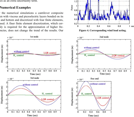
A typical stochastic wind-type load on the side of the structure (Figure 4).
2 2 2 2
1 1
2 2 2 6
1 1
n n n n
n n n n
u
O I
x t x
M K M D
O O
d t q
M M
t u t
M f
t
(27)
In this way we treat uncertainty in the original ma-trices as an extra uncertainty term.
4. Numerical Examples
For the numerical simulations a cantilever composite be
tization, which cer-roximation of higher trend of the results. Our
4.1. Results
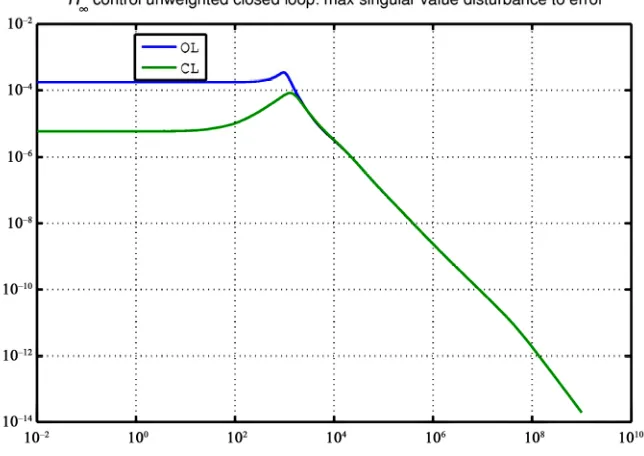
The first load analyzed is sinusoidal load acting on the side of the structure. Figure 5 shows the dynamical re-sponse for the displacements of the uncontrolled and
D
x t Ax t Bu t Gd t G q t
am with viscous and piezoelectric layers bonded on its top and bottom and discretized with four finite elements, is used. A finer finite element discre
tainly is required for the app
quencies, does not change the Figure 4. Corresponding wind load acting.
[image:5.595.69.294.80.298.2]for the displacement with LQR and H∞ control and response without control.
[image:5.595.70.531.319.721.2]controlled beam with LQR control [12,13] and H
control [14,19], for the four nodes of t am. Figure 6
shows the dynamical response for th rotations of the uncontrolled and controlled beam with LQR control and
he be e
H
The beam
control strategy, for the four n of the beam. with
odes
H control keep ilibrium and
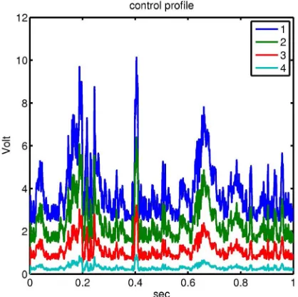
zero ddisplacements, comp bration reduc-tion is achieved. The comparison of the open and closed loop frequency response of the system are shown in Fig-ure 7, as shown in figure, there is a significant improve- ment in the effect of disturbance on error up to the fre-quency of 1000 Hz. Figure 8 shows the control voltages for the four nodes of the beam. The control voltages for
the disturbance rejections of the beam are less than 500 volt.
Comparison with the open loop response for the same plant shows the good performance of the
s in equ lete vi we have
H controller.
Results are very good, and the beam remains in equilib-rium. Reduction of vibrations is observed, while piezo-electric add-ons produce voltage within their tolerance limits (±500 volt).
Then a typical wind load (Figure 4) acting on the side of the structure. The wind load is a real life wind speed measurements in relevance with time that took place in Estavromenos of Heraklion Crete. We transform the wind speed in wind pressure with,
[image:6.595.58.536.253.460.2]or the
Figure 6. Response of the four nodes on the vibrating beam f rotation with LQR and H∞ control and without control.
Figure 7. Singular value for H∞ control strategy.
[image:6.595.138.460.495.723.2]Figure 8. Control profile for the four nodes with H∞ control strategy.
1 2
2
m u
f t C V t (29) where V = velocity, ρ= density and Cu= 1.5.
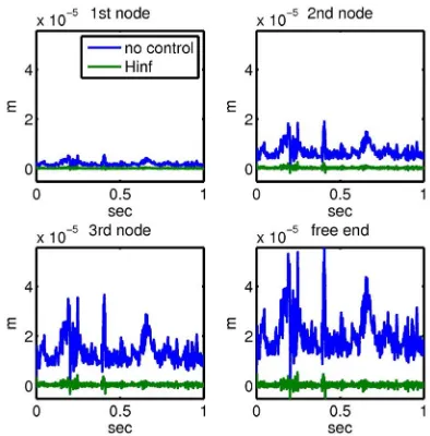
In Figure 9 the structural displacement responses are reported, for the four nodes of the beam. It is possible to see clearly the benefit induced the control on the maxi-mum value of these di ements.
H
splac controller
re-sults are very satisfactory and prove that H control
can reduce smart structures . In Figure 10 we can see the structural r the four nodes of the beam. The m with
vibrations fo rotations
bea H
p
co l keeps in equilibrium and we most zero dis l ents.
In Figure 11 we can see the control profile for the four nodes of the beams. As we can see t
less than 500 Volt, which is the piezo
4.2. Reduced Order Control
The H∞ controller found is of order 24. The fact that
con-troller order, which is equal to the order of the system, is relatively higher than the order of classical controllers such as LQR has led a number of researchers to develop order reduction algorithms. The most widely used such algorithm, known as HIFOO, has been implemented in a Matlab environment, and is the one used in the following procedure [17,20].
The general problem is to compute a controller of re-duced order n < 24 while retaining the performance of the H criterion as well as the behaviour of a full order
ntro acem have al
he voltage is more electric limit.
Figure 9. Responses of the four nodes of the beam without and with H∞ control.
controller for the given system [17,20].
Nonsmooth variation analysis and related computa-tional methods are powerful tools that can be effectively applied to identify local minimizes of nonconvex +optimization problems arising in fixed-order controller design. Our computational methods found a 24th order
controller that stabilized the system. Using the Matlab package HIFOO we can reduce this controller and stabi-lize the system with a 2nd order controller without diffi-
[image:7.595.324.521.387.587.2]Figure 10. Rotations of the four nodes of the beam without and with H∞ control.
Figure 11. Control voltages for the four nodes of the beam using H∞ control.
culty, suggesting explicit formulas for the closed loop system. Furtherm
for the controller and ore, our analytical techniques prove that this controller is locally optimal in the sense that there is no nearby controller with the same order for which the closed loop system has all its poles further left in the complex plane [20].
These approaches can be extended in order to take into account other key quantities of great practical interest, such as optimization of H performance. In particular,
with the help of a MATLAB toolbox called HIFOO (H
Fi
free end of the beam, using hifoo controller (a second order controller). Figure 13 shows the control voltages for the four nodes of the beam [20]. As we can see we need less energy then the 24th controller for reduced
vi-brations.
5. Conclusion
A mathematical formulation and finite element model for the vibration suppression of a cantilever beam with piezo-electric laminated surface and viscous layers and elastic core is presented in this paper. The design of the piezo-electric active control using LQR strategy and
xed Order Optimization) we can reduce the order of the controller and have very good results. Figure 12, shows the response of the uncontrolled and control beam of the
H
con-trol theory for the nominal and damaged sandwich beam has been studied. The numerical results show that the
H control strategy is very effective and suppresses the
vibrations of the beam. The vector of active control forces
Figure 12. Displacement of the free end of the beam without and with hifoo controller.
Figure 13. Control voltages for the four nodes of the beam using hifoo controller.
[image:8.595.68.277.332.540.2] [image:8.595.311.535.517.702.2]subjected to H performance criterion and satisfying
stems dynamic equations such that to reduce the wind excitations is determined. High robust performance and robust stability are achieved. This work clearly dem-onstrates the advantages of using advanced robust control theory for the design of practical smart structure.
6. Acknowledgements
The authors would like to thank the Wind Energy and Synthesis of Energy Systems Laboratory, of the Techno-logical Educational Institute of Crete, for their offer on real life wind speed measurements in relevance with time that took place in Estavromenos of Heraclion Crete.
REFERENCES
[1] K. G. Arvanitis, E. C. Zacharenakis, A. G. Soldatos and
Publishers, Singapore, 2003, pp. 321-415. doi:10.1142/9789812795526_0008
the sy
G. E. Stavroulakis, “New Trends in Optimal Structural Control. Selected Topics in Structronic and Mechatronic System,” World Scientific
[2] G. Foutsitzi, D. Marinova, E. Hadjigeorgiou and G. Stavroulakis, “Robust H2 vi Bration Control of Beams with Piezoelectric Sensors and Actuators,” Proceedings of Physics and Control Conference (PhyCon03), St. Pe-tersburg, Vol. I, 20-22 August 2003, pp. 158-163.
[3] G. Foutsitzi, D. Marinova, E. Hadjigeorgiou and G. Stavroulakis, “Finite Element Modelling of Optimally Controlled Smart Beams,” 28Ih Summer School: Applica-tions of Mathematics in Engineering and Economics, So-zopol, Bulgaria, 2002.
[4] B. Miara, G. Stavroulakis and V. Valente, “Topics on Mathematics for Smart Systems,” Proceedings of the European Conference, Rome, 26-28 October 2006,World Scientific Publishers, Singapore, 2007.
[5] G. E. Stavroulakis, G. Foutsitzi, E. Hadjigeorgiou, D. Marinova and C. C. Baniotopoulos, “Design and Robust Optimal Control of Smart Beams with Application on Vibrations Suppression,” Advances in Engineering Soft-ware, Vol. 36, No. 11-12, 2005, pp. 806-813.
, New York, 1969.
[6] H. F. Tiersten, “Linear Piezoelectric Plate Vibrations,” Plenum Press
[7] N. Zhang and I. Kirpitchenko, “Modelling Dynamics of a Continuous Structure with a Piezoelectric Sensor/Actua- tor for Passive Structural Control,” Journal of Sound and Vibration, Vol. 249, No. 2, 2002, pp. 251-261.
doi:10.1006/jsvi.2001.3792
[8] T. T. Soong and G. D. Manolis. “Active Structures,”
ASCE Journal of StructuralEngineering, Vol. 113, No. 11, 1987, pp. 2290-2302.
doi:10.1061/(ASCE)0733-9445(1987)113:11(2290)
[9] M. D. Symans and M. C. Konstantinou, “Semi-Active Control System for Seismic Protection of Structure: A State-of-the-Art Review,” Engineerings Structures, Vol. 21, No. 6, 1999, pp. 469-487.
doi:10.1016/S0141-0296(97)00225-3
[10] M. Anjanappa and J. Bi, “Magnetostrictive Mini Structures for Smart Structure
Applica-mart Materials andStructures, Vol. 3, No. tors for Smart
tions,” Int. J. S
4, 1994, pp. 383-390. doi:10.1088/0964-1726/3/4/001 [11] K. Chandrashekara and S. Varadarajan, “Adaptive Shape
Control of Composite Beams with Piezoelectric Actua-tors,” Intelligent Materials Systems and Structures 8, 1997, pp112-124e IEEE EMBS, San Francisco, 1-5 Sep-tember 2004, pp. 2758-2761.
[12] O. Bosgra and H. Kwakernaak, “Design Methods for Control Systems,” Course notes, Dutch Institute for Sys-tems and Control, Vol. 67, 2001.
[13] A. Packard, J. Doyle and G. Balas, “Linear, Multivariable Robust Control with a μ Perspective,” ASME Journal of Dynamic Systems, Measurement and Control,50th Anni-versary Issue, Vol. 115, No. 2b, 1994, pp. 310-319. [14] B. A. Francis, “A Course on H∞ Control Theory,” Springer-
Verlag, Berlin, 1985.
[15] J. Friedman and K. Kosmatka, “An Improved Two Node Timoshenko Beam Finite Element,” Computer and Structures, Vol. 47, No. 3, 1993, pp. 473-481.
doi:10.1016/0045-7949(93)90243-7
[16] A. Moutsopoulou, A. Pouliezos and G. E. Stavroulakis, “Modelling with Uncertainty and Robust Control of Smart Beams,” In: B. H. V. Topping and M. Papadra-kakis, Eds., Proceedings of the Ninth International Con-ference on Computational Structures Technology, Paper 35, Civil Comp Press, Stirlingshire Scotland, Civil Comp Press, 2008. doi:10.4203/ccp.88.35
[17] J. V. Burke, D. Henrion and M. L. Lewis, “Overton HI
Control Design, Toulouse, 2006. www.cs.nyu.edu/overton/software/hifoo
[18] C. Sisemore, A. Smaili and R. Houghton, “Passive Damping of Exible Mechanism System: Experimental and Finite Element Investigation,” The 10th World Con-gress of the Theory of Machines and Mechanisms, Oulu, Vol. 5, 1999, pp. 2140-2145.
[19] A. Pouliezos, “Mimo Control Systems,” Class Notes. http://pouliezos.dpem.tuc.gr
[20] J. V. Burke, D. Henron, A. S. Kewis and M. L. Overton, “Stabilization via Nonsmooth, Nonconvex Optimization,”
IEE Automatic Control, Vol. 5, No. 11, 2006, pp. 1760- 1769. doi:10.1109/TAC.2006.884944