ISSN Online: 2161-7198 ISSN Print: 2161-718X
DOI: 10.4236/ojs.2018.81009 Feb. 13, 2018 134 Open Journal of Statistics
Pattern Recognition of Rainfall Using Wavelet
Transform in Bangladesh
Abdur Rahman
1*, Ataul M. Anik
1, Zaki Farhana
1, Sujit Devnath
2, Zobaer Ahmed
31Department of Statistics, Shahjalal University of Science and Technology, Sylhet, Bangladesh 2American International University, Dhaka, Bangladesh
3Ghent University, Gent, Belgium
Abstract
The aim of the study is to explore the regional variation of changing patterns of rainfall in Bangladesh using wavelet transform. The study is completed us-ing rainfall variation of the five regions of Bangladesh as Dhaka, Cox’s Bazar, Rajshahi, Bogra and Sylhet. The duration of the study period was 69 years for Dhaka, 64 years for Cox’s Bazar, 40 years for Rajshahi, 54 years for Bogra and 55 years for Sylhet. The results of the wavelet analysis reveals that, in Rajshahi the amount of rainfall are decreasing in a significant rate among the other study regions. It also explores the annual periodicity of rainfall for all the study regions along with a special 6-month periodicity in the Cox’s Bazar. In addition, this analysis also explores a dominating 3 - 4 year cycle of rainfall in all the study regions. Besides the climate change in Cox’s Bazar and Sylhet are pretty much alarming.
Keywords
Wavelet Analysis, Rainfall, Regional Variation, Bangladesh
1. Introduction
The wavelet transform has attracted much attention in 1984 when Grossman and Morlet developed a theoretical explanation; it is generally used in signal processing [1]. This has an advantage over classical spectral analysis because it allows analyzing different scales of temporal variability and does not need a sta-tionary series as well as a common tool to measure the variations of power within a given data. Some areas of wavelet transform are data compression, nuc-lear engineering, signal and image processing, geophysics and pure mathematics and also in the dispersion of ocean waves, wave growth and breaking, structures
How to cite this paper: Rahman, A., Anik, A.M., Farhana, Z., Devnath, S. and Ahmed, Z. (2018) Pattern Recognition of Rainfall Using Wavelet Transform in Bangladesh. Open Journal of Statistics, 8, 134-145. https://doi.org/10.4236/ojs.2018.81009
Received: November 30, 2017 Accepted: February 10, 2018 Published: February 13, 2018
Copyright © 2018 by authors and Scientific Research Publishing Inc. This work is licensed under the Creative Commons Attribution International License (CC BY 4.0).
DOI: 10.4236/ojs.2018.81009 135 Open Journal of Statistics
in turbulent flows and stream flow characterization [2] [3] [4] [5]. Wavelet transforms are multi resolution representations of signals and images. They de-compose signals and images into multi scale details [6][7][8]. Wavelet expan-sions can describe sharp transitions in images preserved and depicted extremely well [8]. This special treatment of edges by wavelet transform is very attractive in image filtering. At large scales, the filter we are exploring, pass essentially all the signals. However the signal at small scales reduces noise preferentially. To keep the edges sharp, small-scale information is required. If the small-scale data is passing around identified edges, noise is reduced and the identified edges stay sharp. The main key to this technique is to just identity the edges. The small- scale data is passed at positions where the correlation is large and suppressed if the correlation is small.
Bangladesh is one of the most vulnerable countries in the world due to climate change. To overcome the uncertainties it is necessary to evaluate the spatial and temporal changes that have already occurred in our past climate of Bangladesh. However, there don’t seem to be enough studies that are drained this respect to an enormous body of literature that is on the market on future climates from model predictions. Ahmed et al. (1992) [9] studied the trends in annual rainfalls of Asian nation. They over that there was no important trend within the annual rain over the country. Ahmad et al. (1996) [9] report a rise of 0.5˚C in tempera-ture over Asian nation throughout past one hundred years. Rahman et al. (1997)
[10] studied the semi-permanent monsoonal rain pattern at twelve stations of Asian nations, they found no overall trend in seasonal total rain, they detected some trends in monthly rainfalls of the 2 extremely urbanized stations (Dhaka and Chittagong). Mondal associate degreed Wasimi (2004) [11] analyzed the temperatures and rainfalls of the Ganges River Delta at intervals Asian nation and located an increasing trend of 0.5˚C and 1.1˚C per century in day-time most and night-time minimum temperatures, severally. They additionally analyzed seasonal rainfalls of the delta. Their results showed increasing trends in winter, pre-monsoon and summer rainfalls, there was no considerable overall trend in essential amount rain. Supported regional trends in temperatures and rainfalls, they over that the water inadequacy within the time of year may increase and therefore the essential amount may become a lot of essential in future. SAARC meteoric analysis Centre (SMRC, 2003) [12] studied surface climatological in-formation on monthly and annual mean most and minimum temperatures, and monthly and annual rainfalls for the amount of 1961-1990. The study showed associate degree increasing trend of mean most and minimum temperatures in some seasons and decreasing trend in some others. A. Rahman et al. (2015) [13]
Centi-DOI: 10.4236/ojs.2018.81009 136 Open Journal of Statistics
grade per annum. Overall, the trend of the annual mean most temperature had shown a major increase over the amount of 1961-1990. Rahman and Alam (2003) [14] found that the temperature was typically increasing within the June-August amount. Average most associate degreed minimum temperatures showed an increasing trend of 5˚C and 3˚C per century, severally. On the oppo-site hand, average most and minimum temperatures of December-February amount showed, severally, a decreasing associate degreed an increasing trend of 0.1˚C and 1.6˚C per century. Regional variations had additionally been ascer-tained round the average trend (SMRC, 2003) [4]. In a very recent study, global climate change Cell (2009) [15] had analyzed the temperature and sunshine length in the least BMD stations of Asian nation. It had additionally analyzed rain trend at eight stations. Rain information at alternative stations couldn't be analyzed attributable to time and monetary fund limitations and therefore the rain information once the year of 2001 weren't offered for the study. Islam and Neelim (2010) [16] analyzed the most and minimum temperatures of 4 months (January, April, could and December) and 2 seasons solely months of April-May were thought-about because the summer season and therefore the two months of December-January because the winter season within the study. The study found normally associate degree increasing trend in each summer and winter tempera-tures. The rain information of some designated locations were additionally studied by Islam and Neelim (2010) [16]. However, they didn’t build any complete as-sessment of trend in rain in several time scales. Most of their analyses were on straightforward distribution of rain in a very kind of bar graphs.
2. Data
The study deals with rainfall over five weather station of BMD (Bangladesh Me-teorological Department) from five different regions of Bangladesh defined by Cox’s Bazar (South-Eastern zone), Sylhet (North-Eastern zone), Bogra (North- Western zone), Rajshahi (Western zone) and Dhaka (South-Central zone). The reasons behind selecting these stations are availability of the long-time data, minimum missing observations and covering almost all topological region of Bangladesh. The data for this study has been collected from Bangladesh Meteo-rological Department (BMD) which is the authorized government organization for meteorological activities of Bangladesh. The duration of the study period was chosen as 1953-2012 for Dhaka, 1948-2012 for Cox’s Bazar, 1972-2012 for Raj-shahi, 1958-2012 for Bogra and 1957-2012 for Sylhet.
3. Methodology
DOI: 10.4236/ojs.2018.81009 137 Open Journal of Statistics
sliding it along with time. It computes the Fast Fourier Transform (FFT) every time using the only data within given window size which solves the frequency localization problem. But in case of inconsistent treatment frequencies there are some problems in WFT like in case of low frequencies there are so few oscilla-tions in the window that the frequency localization is lost. Meanwhile at high frequencies there are so many high oscillations that the time localization is lost. To measure the stationarity of a time series it is necessary to calculate the run-ning variance using fixed width window. Though there are some disadvantages using a fixed width window but still the analysis could be repeated with a variety of window widths. To solve this problem Wavelet Transform can be used, which transformed or decomposed a one dimensional time series into two diffusive time series simultaneously. Only then it is possible to get information from any periodic signals within the time series and how this time series varies over time [17].
Morlet wavelet is nothing more than a sine wave which is multiplied by a Gaussian envelope. If the width of the wavelet is 10 years then it is possible to find the correlations of the curve. Thus a single number gives a measure of the projection of this wave packet on the data during the different period in different region. A new time series of the projection amplitude versus time can be con-structed by sliding this wavelet along the time series. The scale of the wavelet can be varied by changing its width and thus it is more preferable than a moving Fourier Spectrum. In wavelet analysis a same shape of wavelet is use only the size scales up or down depending with the window size. In application, the Morlet wavelet is defined as the product of a complex exponential wave and a Gaussian envelope [1][2][3][4][5][17]:
( )
2 1
4 2
0 π e e
i o
η ω η
ψ η = − − (1)
where, ψ η0
( )
is the wavelet value at non-dimensional time η and ω0 is thenon-dimensional frequency, equal to 6 in this study to satisfy an admissibility condition; i.e., the function must have zero mean and be localized in both time and frequency space to be admissible as a wavelet. This is the basic wavelet func-tion, but we need to change this wavelet along in time. Thus, the scaled wavelets are defined as,
(
)
1 2(
)
0
n n t t n n t
s s s
δ δ δ
ψ ′− = ψ ′−
(2)
where s is the dilation parameter is used to change the scale, and 𝑛𝑛 is the trans-lation parameter used to slide in time [17]. The wavelet transforms W sn
( )
isjust the inner product of the wavelet function with the original time series [18] [19][20][21][22],
( )
1(
)
*
0 N
n n
n
n n t
W s x
s δ ψ − ′ ′= ′ − =
∑
(3)DOI: 10.4236/ojs.2018.81009 138 Open Journal of Statistics
dates. A two-dimensional picture of the variability can then be constructed by plotting the wavelet amplitude and phase. Then, a time series can be decom-posed into time-frequency phase space using a typical (mother) wavelet. The actual computation of the wavelet transform can be done by the following algo-rithm [23]: 1) choose a mother wavelet; 2) find the FT of the mother wavelet; 3) find the FT of the time series; 4) choose a minimum scale so, and all other scales; 5) for each scale, do:
a) Using Equation (4), or whatever is appropriate for the mother wavelet in use, compute the daughter wavelet at that scale:
(
)
1 2 0(
)
2π ˆ k k s s s t
ψ ω ψ ω
δ
= (4)
where ψˆ0 indicate the FT.
b) Normalize the daughter wavelet by dividing by the square-root of the total variance;
c) Multiply by the FT of time series;
d) Using Equation (5), inverse transform back to real space;
( )
1( )
* 0
ˆ
ˆ e k
N
i n t
n k k
k
W s x
ψ
sω
ω δ−
=
=
∑
(5)where, ωk is the angular frequency, equal to 2πk N tδ for k≤N 2 or equal
to −2πk N tδ for k>N 2. It is possible to compute the wavelet transform in
the time domain using Equation (3). However, it is much simpler to use the fact that the wavelet transform is the convolution between the two functions 𝑥𝑥 and
𝜓𝜓, and to carry out the wavelet transform in Fourier space using the FFT; and e) make a contour plot.
4. Results and Discussions
Wavelet spectra for the length of the study amount was chosen as 1953-2012 for national capital, 1948-2012 for Cox’s Bazar, 1972-2012 for Rajshahi, 1958-2012 for Bogra and 1957-2012 for Sylhet square measure showing Figures 1-5. we elect wave analysis as a result of, applications like normal Fourier remodel anal-ysis to a statistic ought to be solely tried once the statistic fulfils 2 vital characte-ristics as, stationary and also the statistic will be delineated because the summa-tion of various amounted elements (described by straightforward harmonic functions) for the total period. However, most statistic from meteorology don't fulfil each necessities. Ultimately, earth sciences statistic square measure typical-ly no stationary. Several hydrological statistic, like precipitation, gift unregulartypical-ly distributed events with no stationary power over many various frequencies. Thus, their intrinsic temporal structure isn't well delineated by the superposition of a number of frequency elements as derived during a usual analysis.
4.1. Wavelet Power Spectrum
DOI: 10.4236/ojs.2018.81009 139 Open Journal of Statistics
analysis are set as δt=1 month and so=2 months because s=2δt, 0.25
j
δ
= to do 4 sub octaves per octave, and 1 7j j
δ
= in order to do 7
pow-ers-f-two with δj sub octaves each.
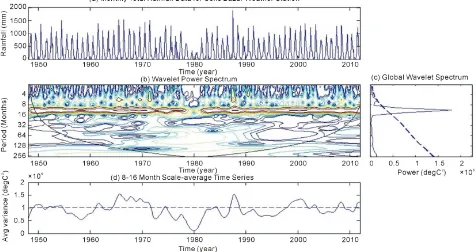
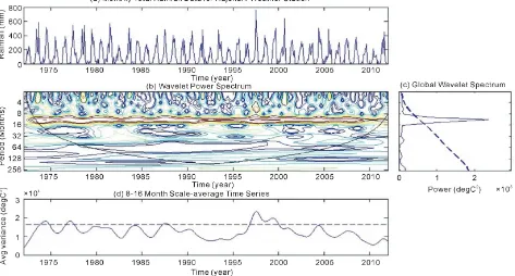
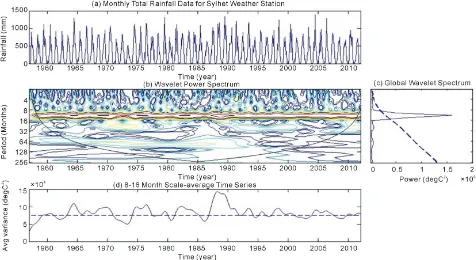
Figures 1(b)-5(b) shows the power (absolute value squared) of the wavelet transform for the monthly rainfall in different regions of Bangladesh presented in Figures 1(a)-5(a). As declared before, the (absolute value square) offers info on the relative power at an explicit scale and an explicit time that shows the par-ticular oscillations of the individual wavelets, instead of simply their magnitude.
Observing Figures 1(b)-5(b), it is clear that there are more concentration of power between the 8 - 16-months band which shows that this time series has a strong annual signal in cox’s bazar. Wavelet power spectrum at 95% significant level presents an important peak for precipitation episodes with characteristic scale of 2 - 4-months. The variance of power in 8 - 16-month band (also con-firmed later by Figures 1(d)-5(d)) also shows the dry and wet years which means when the power decreases substantially it means a dry year similarly for the maximum of power it is a wet year. In the years 1985 and between the years 2006 to 2009 an extreme increase in power can be found which corresponds Dhaka region has a wet year. Since 1956 and between1990 to 2004 a dry period that contains certain reductions can be identified. Errors have occur at the be-ginning and end of the wavelet power spectrum because we are dealing with fi-nite-length time series. We can get rid of that problem by padding the end of the time series with zero before applying the wavelet transform and then remove them afterward. Amplitude decreases near the edges since we pad the time series with zero which introduces discontinuities. The amplitude decreases conti-nuously as the more zero enter the analysis. The region of the wavelet spectrum in which edge effects is essential as it is defined as the e-folding time for the au-tocorrelation of wavelet power at each scale. The peaks of these regions have been reduced in magnitude while padding zero. Thus it is quite unclear that the decrease in cross-hatched region is a true decrease or an artifact of the padding. We don’t need to pad with zeroes for cyclic series. The black contour in the same figure is the 95% significance level, using a red-noise background spectrum. Un-ivariate lag-1 autoregressive process is a simple model for red noise. The correla-tion between the time series and itself is the lag-1 but shifted (or lagged) by one time unit. In this study this shift is one month. Persistent of an anomaly is measured by the lag-1 from one month to the next. The true lag-1 can be com-puted by an approximation using
(
1/2)
1 2 2
α= α α , where α1 is the lag-1
auto-correlation and 𝛼𝛼2 is the lag-2 autocorrelation, which is the same as lag-1 but just
shifted by two points instead of one. Figures 1(b)-5(b) and Figures 1(c)-5(c)
DOI: 10.4236/ojs.2018.81009 140 Open Journal of Statistics
Figure 1. (a) Monthly rainfall in Dhaka for 1953-2012; (b) The wavelet power spectrum using Morlet mother wavelet; (c) The global wavelet power spectrum. The dashed line indicates 5% significance level for the global wavelet spectrum; and (d) Scale- average wavelet power over the 8 - 16 months’ band. The dashed line is the 95% confidence. Wavelet power decreases according to the following order: red, orange, yellow, blue and white.
[image:7.595.61.537.414.666.2]DOI: 10.4236/ojs.2018.81009 141 Open Journal of Statistics
Figure 3. (a) Monthly rainfall in Bogra for 1953-2012; (b) The wavelet power spectrum using Morlet mother wavelet; (c) The global wavelet power spectrum. The dashed line is the 5% significance level for the global wavelet spectrum; and (d) Scale-average wavelet power over the 8 - 16 months’ band. The dashed line is the 95% confidence. Wavelet power decreases according to the following order: red, orange, yellow, blue and white.
[image:8.595.63.536.414.668.2]DOI: 10.4236/ojs.2018.81009 142 Open Journal of Statistics
Figure 5. (a) Monthly rainfall in Sylhet for 1953-2012; (b) The wavelet power spectrum using Morlet mother wavelet; (c) The global wavelet power spectrum. The dashed line is the 5% significance level for the global wavelet spectrum; and (d) Scale-average wavelet power over the 8 - 16 months’ band. The dashed line is the 95% confidence. Wavelet power decreases according to the following order: red, orange, yellow, blue and white.
4.2. Global Wavelet Power Spectrum
Figures 1(c)-5(c) shows the annual frequency of this time series is confirmed by an integration of power over time which shows only one significant peak above the 95% Confidence level for the global wavelet spectrum assuming white-noise (Figures 1(b)-5(b)) represented by the dashed lines. In Figures 1(c)-5(c)
presents an almost significant peak (at the 95% level) centered in the 2 - 4- month band. The most extreme monthly precipitation values for different re-gions of Bangladesh (values above 500 mm in Figure 1(a), 1000 mm in Figure 2(a), 400 mm in Figure 3(a), 200 mm in Figure 4(a) and 1000 mm in Figure 5(a)) correspond to pulses of highly significant power within the 2 - 4-month band (Figures 1(b)-5(b)). We used global wavelet spectrum because it provides an unbiased and consistent estimation of the true power spectrum of the time series and a simple and robust way to characterize the time series variability. Global wavelet spectrum is useful for summarizing a region's temporal variabili-ty and comparing it other regions that does not display long-term changes in hyetograph structures.
4.3. Scale-Average Time Series
frequen-DOI: 10.4236/ojs.2018.81009 143 Open Journal of Statistics
cy by another within the same time series. Figures 1(b)-5(b) made averaging all scales between 8 and 16 months, which gives us a measure of the average year variance versus time. In Dhaka region, in 1985 and between the year 2006 to 2009 corresponds to a wet year and dry period that contains certain reductions can be identified in 1956 and between 1990 to 2004 and after that it was wet pe-riod. In Cox’s Bazar region 1958 and 1960 corresponds to a dry period and years 1965 to 1970, 1988 and 1999 to 2001 corresponds most wet period. In Bogra re-gion, year 1978 to 80, 1988 and 1999 corresponds to wet period and other years corresponds to dry period. In Rajshahi region only in 1998 corresponds to wet period and almost all year it extremely dry period. In Sylhet region, only 1979 and 1986 corresponds to dry period and all the year corresponds to wet period.
5. Conclusion
Climate change in Bangladesh got tremendous momentum since the advent of 90’s in terms of rainfall. The adverse impact of this climate change in Rajshahi region has become the most vulnerable region and this process continues at an increasing rate. Cox’s Bazar and Sylhet region are also in an alarming position. The findings of this study show that Bangladesh is a vulnerable country to cli-mate change in terms of rainfall. Dialogues at both national and international levels should be launched in different forums to ameliorate the adverse factors of climate change. To produce more authentic findings for policy implications, further comprehensive and appropriate research can be undertaken and imple-mented in this very field.
Acknowledgements
We thank the Bangladesh Meteorological Department (BMD) for providing the data which is the authorized government organization for meteorological activi-ties of Bangladesh.
Conflict of Interest
We declare that there is no conflict of interest.
References
[1] Grossman, A. and Morlet, J. (1984) Decomposition of Hardy Functions into Square Integrable Wavelets of Constant Shape. SIAM Journal on Mathematical Analysis, 15, 723-736. https://doi.org/10.1137/0515056
[2] Graps, A. (1995) An Introduction to Wavelets. IEEE Computational Science and Engineering, 2, 50-61. https://doi.org/10.1109/99.388960
[3] Torrence, C. and Compo, G.P. (1998) A Practical Guide to Wavelet Analysis. Bulle-tin of the American Meteorological Society, 79, 61-78.
https://doi.org/10.1175/1520-0477(1998)079<0061:APGTWA>2.0.CO;2
[4] Farge, M. (1992) Wavelet Transforms and Their Applications to Turbulence. An-nual Review of Fluid Mechanics, 24, 395-457.
DOI: 10.4236/ojs.2018.81009 144 Open Journal of Statistics
[5] Smith, L.C., Turcitte, D.L. and Isacks, B.L. (1998) Stream Flow Characterization and Feature Detection Using a Discrete Wavelet Transform. Hydrological Processes, 12, 233-249.
https://doi.org/10.1002/(SICI)1099-1085(199802)12:2<233::AID-HYP573>3.0.CO;2-3
[6] Daubechies, I. (1998) Orthonormal Bases of Compactly Supported Wavelets.
Communications on Pure and Applied Mathematics, 41, 909-996.
https://doi.org/10.1002/cpa.3160410705
[7] Mallat, S.G. (1989) A Theory for Multiresolution Signal Decomposition the Wavelet Representation. IEEE Transactions on Pattern Analysis and Machine Intelligence, 11, 674-693. https://doi.org/10.1109/34.192463
[8] Mallat, S.G. and Zhong, S. (1989) Complete Signal Representation with Multiscale Edge. NYU Tech Rep. No. 483.
[9] Ahmed, S.M.U., Hoque, M.M. and Hussain, S. (1992) Floods in Bangladesh: A Hy-drological Analysis. Final Report No. R01/92, IWFM, BUET.
[10] Rahman, M.R., Salehin, M. and Matsumoto, J. (1997) Trend of Monsoon Rainfall Pattern in Bangladesh. Bangladesh Journal of Water Resources Research, 14-18, 121-138.
[11] Mondal, M.S. and Wasimi, S.A. (2004) Impact of Climate Change on Dry Season Water Demand in the Ganges Delta of Bangladesh. In: Rahman, M.M., Alam, M.J.B., Ali, M.A., Ali, M. and Vairavamoorthy, K., Eds., Contemporary Environ-mental Challenges, CERM, ITN, BUET, WEDC, IDE and Loughborough Universi-ty, 63-83.
[12] SMRC (2003) The Vulnerability Assessment of the SAARC Coastal Region Due to Sea Level Rise: Bangladesh Case. SAARC Meteorological Research Centre, Dhaka. [13] Rahman, A., Jiban, J.H.M. and Munna, S.A. (2015) Regional Variation of
Tempera-ture and Rainfall in Bangladesh: Estimation of Trend. Open Journal of Statistics, 5, 652-657.https://doi.org/10.4236/ojs.2015.57066
[14] Rahman, A. and Alam, M. (2003) Mainstreaming Adaptation to Climate Change in Least Developed Countries (LDCs). Working Paper 2: Bangladesh Country Case Study, IIED, London.
[15] Climate Change Cell (2009) Characterizing Long-Term Changes of Bangladesh Climate in Context of Agriculture and Irrigation. Department of Environment, Dhaka.
[16] Islam, T. and Neelim, A. (2010) Climate Change in Bangladesh: A Closer Look into Temperature and Rainfall Data. The University Press Limited, Dhaka.
[17] Santos, C.A.G., Galvao, C.O., Suzuki, K. and Trigo, R.M. (2001) Matsuyama City Rainfall Data Analysis using Wavelet Transform. Annual Journal of Hydraulic En-gineering, 45, 211-216.
[18] McVeigh, E.R., Honkelman, R.M. and Bronskill, M.J. (1985) Noise and Filtration in Magnetic Resonance Imaging. Medical Physics, 12, 586-591.
https://doi.org/10.1118/1.595679
[19] Hart, H. and Liang, Z. (1988) Bayesian Image Processing in Two Dimensions. IEEE Transactions on Medical Imaging, 6, 201-208.
https://doi.org/10.1109/TMI.1987.4307828
[20] Hu, X., Johnson, V., Wong, W.H. and Chen, C.-T. (1991) Bayesian Image Pro- cessing in Magnetic Resonance Imaging. Magnetic Resonance Imaging, 9, 611-620.
https://doi.org/10.1016/0730-725X(91)90049-R
DOI: 10.4236/ojs.2018.81009 145 Open Journal of Statistics
Images with Wavelet Transforms. Magnetic Resonance in Medicine, 21, 288-295.
https://doi.org/10.1002/mrm.1910210213
[22] Xu, Y., Lu, J., Healy, D.M. and Weaver, J.B. (1991) Filtering MR Images with Wave-let Transforms. 199.
[23] Torrence, C. and Compo, G.P. (1998) A Practical Guide to Wavelet Analysis. Bulle-tin of the American Meteorological Society, 79, 61-78.