Inverse methods and modelling

INVERSE METHODS AND MODELLING

A thesis

presented fo~ the Degree of

Doctor of Philosophy in Electrical Engineering in the

University of Canterbury, Christchurch, New Zealand

by

R,P.

MILLANE

University of Canterbury 1981

ABSTRACT

Three applications of inverse methods are considered,

The theoretical bases of the or inverse scattering techniques used to the interior of penetrable bodies are reviewed

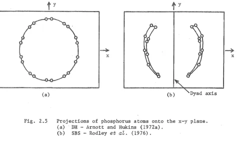
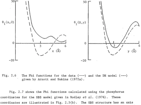
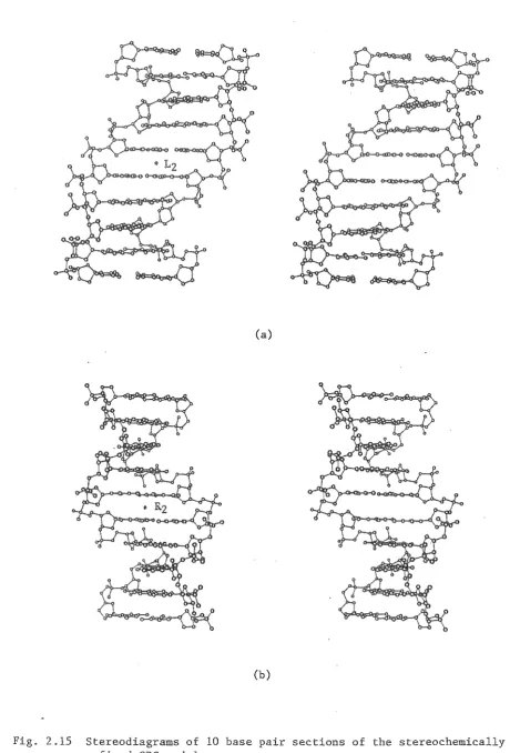
X-ray crystallography is used to the molecular structure of crystals. Two models of the DNA molecule are analysed on the basis of the X-ray diffraction data. The two models are the widely accepted "double helix" and the recently proposed "side-by-side". It is shown that the side-by-side model fits the diffraction data at least as well as the double helix. A stereochemical analysis shows that the side-by-side model is also stereochemically acceptable.

Current methods. for imaging regions of variable refractive index are useful only for weak inhomogeneities, A time domain method for imaging one-dimensional regions of arbitrary variation in refractive index is outlined. It is shown that this method may be applied to. branched transmission line networks. These techniques are applied to both simulated and measured data.

Physiological and clinical aspects of cardiac arrhythmias are reviewed.

A modelling approach to the inverse ?roblem of cardiac arrhythmia

diagnosis is outlined. The important variables describing cardiac conduction are identified and used as· the basis of an interactive computer

model to assist in arrhythmia diagnosis. It is shown that the model can simulate realistic quantitative rhythms, Methods of processing patients' clinical data to identify the model parameters are described. Examples of the use of the model to simulate two patients' arrhythmias are

ACKNOWLEDGEMENTS

I sincerely thank my supervisor, Professor Richard Bates, for his continual encouragement and guidance throughout the course of the work reported in this thesis.

Special thanks are also due to Dr Gordon Rodley and Phil Bones for their considerable assistance with the work reported in chapters 2 and 5 respectively.

My colleagues from the Electrical Engineering Department, in particular Dr Graeme McKinnon, Dr Patrick Heffernan, Brent Robinson, Andrew Seagar and Richard Fright, all provided companionship and assistance.

I would also like to thank Dr Allan McKinnon, Robin McNeil,

Adrian Coronno, Gillian Rodley, Marie Flewellen, Dr Andy Maslowski and Dr Hamid Ikram, all of whom have made a contribution to this thesis.

I am grateful to my family, Stephanie Morris, Kathy McSweeney and my friends and flatmates over the years for their support and for helping to keep me sane.

PREFACE

Direct observation of a physical system is often either undesirable, impracticable or impossible. In such a circumstance one must resort to indirect measurement schemes which involve the measurement of quantities related to those required, rather than those quantities themselves. These indirect measurement methods often fall within the realm of inverse

problems. Inverse problems usually involve the determination of the cause of a phenomenon, given a measurement of its effect. Direct problems, on the other hand, generally involve the determination of an effect, given the cause. Inverse problems are, in general, significantly less well understood than the corresponding direct problems.

This thesis is concerned with three applications of inverse methods. Two of these (chapters 1 to 3) fall within the realm of "inverse scattering" which involves the determination of some of the properties of an object from measurement of radiation scattered by it. The third application (chapters 4 and 5) is concerned with physiological modelling to assist in the inverse problem of cardiac arrhythmia diagnosis. Review material is presented in chapters 1 and 4, and original work is reported in chapters 2, 3 and 5.

Chapter 1 contains most of the theoretical preliminaries required for chapters 2 and 3, and reviews the major inverse scattering techniques for imaging the interior of penetrable bodies. The chapter begins with

derivations of the equations describing electromagnetic and acoustic waves in unbounded space and on guiding structures. This is followed by a

description of the major inverse scattering techniques used in imaging, crystallography, echo-location, sounding and profile inversion.

X-ray crystallography is an inverse scattering technique,used to image the molecular structure of crystals from measurement of their X-ray

vi.

see how well it agrees with that observed. Adjustments are made to the model in an attempt to reduce the discrepancy between the calculated and observed diffraction patterns below an acceptable level. Chapter 2 describes the comparison of a new model for DNA (proposed by Dr Gordon Rodley of the Chemistry department of this University) with the accepted double helix model in terms of the observed X-ray diffraction data. A stereochemical assessment of Rodley's model is also described.

Most practical inverse scattering techniques used to image regions of variable refractive index provide useful results only if there is no need to go beyond simple echo-location principles. These methods are unsuitable for imaging inhomogeneities which are either strong or are of spatial extent which is large in comparison to the wavelength of the radiation. In chapter 3 a method, formulated in the time domain, for imaging plane stratified regions with arbitrary variations in refractive index is described. This method is inherently unstable and data

pre-processing procedures. are described which maximise the stability of the algorithm. Examples of applications to both simulated and measured data are presented. The effects of signal bandwidth and measurement noise are discussed as are the improvements in reconstructions over those which are based on simple echo-location ideas. Applications, with examples, of the technique to branched transmission line networks are also described. The time domain method is discussed in relation to the Gelfand-Levitan technique and the inverse normal mode problem.

Chapter 4 serves as an introduction to chapter 5 and reviews cardiac electrophysiology, cardiac arrhythmias and the clinical measurements which are used to assist in arrhythmia diagnosis.

Cardiac arrhythmias are sometimes life threatening and are often

difficult to diagnose. The inverse problem in cardiac arrhythmia diagnosis is to determine the mechanism and phYSiological basis of an arrhythmia from measurements of the surface and intracardiac electrocardiograms under

various conditions. Because cardiac rhythm processes are so complex and the amount of clinical data measured is relatively small, it is often not possible for a cardiologist to find a unique mechanism for an arrhythmia. When a system is complex and the data obtained is sparse, inverse problems can usually only be usefully solved by model fitting procedures • . Modelling provides a convenient way of including the available

a priori

knowledge in the solution. Chapter 5 describes a modelling approach to arrhythmia

impulses (which control heart rhythm) in the cardiac conduction system are identified. These are used as the basis of an interactive computer model of the conduction system which a cardiologist can use to assist in arrhythmia diagnosis. Means of estimating the model from clinical data are described. Examples of the use of the model to

simulate patients' arrhythmias are

The thesis concludes with chapter 6, which presents conclusions and suggestions for future research.

During the course of the work reported in this thesis the following papers and presentations have been

R,H.T. Bates, G.C. McKinnon and R,P. Mlilane, Conformations of DNA Compatible with Available Diffraction Data, Presented at the Sci. ~Ieeting of the Christchurch Med, Res. Soc., Christchurch, N.Z., July 1978. Abstract: N.Z. Med. J. (1979), ~, 190. R.H.T. Bates, G.C. McKinnon and R.P. Millane, A New Look at B-DNA

Diffraction Data, Research Report~ Electrical Engineering Dept., University of Canterbury, N.Z., Nov. 1978.

R.H.T. Bates, G.C. McKinnon, R.P. Millane and G.A. Rodley, Revised Interpretations of the Available X-ray Data for B-DNA, Pramana

(1980), ~, 233-252.

R.P. Millane and P.J. Bones, A Computer Model of the Cardiac Specialised Conduction System. Presented at the 20th Conf. on Phys. Sci. and Eng. in Med. and BioI., Christchurch, N.Z., Aug. 1980. Abstract: Conf. Proc., p. 37.

R.P. Millane, P.J. Bones, H. Ikram and R.H.T. Bates, Use of a Computer Model to Assist in the Diagnosis of Cardiac Arrhythmias,

Presented at the Ann. Sci. Meeting of the Cardiac Soc. of Australia and New Zealand, Dunedin, N.Z., Sept. 1980. Abstract: N.Z. Med. J. (1980), ~. 404.

R.P. Millane, P.J. Bones, H. Ikram and R.H.T. Bates, A Computer Model of Cardiac Conduction, Australasian Phys. . Sci. Med. (1980),

1,

205~209.

viii.

R.P. Millane and G.A. Rodley, Stereochemical Details of the Side-by-Side Model for DNA, Nucleic Acids Res. (1981), 1765-1773.

R.P. Millane and R.H.T. Bates, Inverse Methods for Branched Ducts and Transmission Lines, Proc. lEE on Communications, Radar and

Processing (1981), in press.

R.P. Millane, P.J. Bones, H. Flewellen, H. Ikram and R.H.T. Bates, Possible Mechanisms for two Variants of the Wolff-Parkinson-White Syndrome Suggested by Computer Modelling, Presented at the Sci. Meeting of the Christchurch Med. Res. Soc., Christchurch, N.Z., Nov. 1981.

R.P, btillane, G.A. Radley and G.F. Radley, Refinement of the Side-by-Side Model for DNA, J. Roy. Soc. N,Z. (1982), in press.

G.A. Rodley, R.P. Millane, G.C. McKinnon and R.H.T. Bates, Use of Axial Pattersons in Assessment of Compatibility of Alternative B-DNA

Structures with Fibre X-ray Data, submitted to J. Mol. Biol. (1981). J.H.T. Bates, W.R. Fright, R.P. Mlliane, A.D. Seagar, A.E. McKinnon and

R.H.T. Bates, Subtractive Image Restoration III: Some Practical Applications, to be submitted to Optik (1982).

ABSTRACT

ACKNOWLEDGEMENTS PREFACE

TABLE OF CONTENTS

CHAPTER 1. INVERSE SCATTERING 1.1 Introduction

1.2 Electromagnetic Scattering 1.3 Acoustic Scattering

1.4 Waves in Ducts and Transmission Lines

i iii v 1 1 4 7 8

1.4.1 Electromagnetic Waves on Transmission Lines 8

1,4.2 Sound Waves in Ducts 10

1.5 1.6 1.7

1.8 1.9

The Born Inverse Scattering Approximation The Rytov Inverse Scattering Approximation X-ray Crystallography

1.7.1 X-rays arid Molecular Structure 1.7.2 Diffraction by Crystals

1.7.3 Structure Determination 1.7.4 Structure Refinement

Bates' Solution to the Inverse Scattering Problem The Gelfand-Levitan Technique

1. 9.1 The Schrodinger Equation and the Scattering Matrix

1.9.2 The Chandrasekhar Transform 1.9.3 The Gelfand-Levitan Equation 1.10 The Inverse Eigenvalue Problem 1.11 The Backus and Gilbert Method 1.12 Summary

CHAPTER 2. THE STRUCTURE OF DNA 2.1 Introduction

2.2 Paracrystalline Analysis 2.3 Fibre Analysis

2.4 Stereochemical Refinement 2.5 Axial Pattersons

2.6 Discussion

CHAPTER 3. 3.1 3.2 3.3

3.4

3.5 3.6 3.7

CHAPTER 4. 4.1 4.2

4.3

4.4

4.5 CHAPTER 5.

5.1 5.2 5.3 5.4 5.5 5.6

CHAPTER 6. 6.1

6.2

6.3

APPENDIX 1 APPENDIX 2 APPENDIX 3 APPENDIX 4

REFERENCES

x,

SOME ASPECTS OF EXACT MACROSCOPIC INVERSE SCATTERING Introduction

Time Domain Macroscopic Inverse Scattering Data Pre-processing

Examples of Time Domain Inverse Scattering Branched Networks

Solutions to the Inverse Eigenvalue Problem Discussion

C.~IAC ELECTROPHYSIOLOGY Introduction

Cardiac Physiology Cardiac Arrhythmias The Electrocardiogram

Intracardiac Electrocardiography MODELLING CARDIAC ARRHYTHMIAS Introduction

Modelling Cardiac Conduction Implementation of the Model

Processing Measured Electrophysiological Data Examples

)

5.5.1 The Wolff-Parkinson-White Syndrome

5.5.2 Patient 1

5.5.3 Patient 2

5.5.4 Comments on the Examples

Discussion

CONCLUSIONS AND SUGGESTIONS FOR FUTURE RESEARCH The Structure of DNA

Macroscopic Inverse Scattering

Cardiac Electrophysiolo Modelling Deconvolution Methods

Time Domain Reflectometer Experiments Branched Networks

A Power Series Formulation of the Inverse Eigenvalue Problem

1, INVERSE SCATTERING

1.1 INTRODUCTION

In many situations of scientific and technical importance, direct observation of a physical system is either impossible or impracticable. In such cases one often wishes to determine the properties of a system from a remote location, Problems of this sort are variously referred to as imaging, remote probing or non-invasive measurement, and they all lie within the realm of inverse problems. The term "inverse problems" is used to distinguish them from If one knows the properties of a and the stimulus applied to it, the direct problem consists of determining the system's response, However in a typical inverse problem, the response of the system to a known stimulus is measured and as many as possible of the system properties are to be determined.

Inverse problems are generally more difficult mathematically,

computationally and conceptually than the corresponding direct problems. One of the main reasons for the conceptual difficulty is that they reverse our classical notion of cause and effect. Many inverse problems belong to the class of improperly-posed problems (Deschamps and Cabayan, 1972) in which the solution may depend uniquely but not continuously on the data. Small errors in the data can lead to large errors in the solution unless particular care is taken. Experimental data inevitably contains errors and noise, so this feature of inverse problems is important in practical situations.

In many imaging applications, wave-like radiation is used to probe the unkno,Yn system. By measuring the resulting radiation field, one hopes to determine some of the of the system. Obviously the

interaction between the system and the radiation must be a function of these properties in order for them to be imaged. Inverse problems of this type, involving measurement of the scattering (diffraction) of radiation _, by material bodies (scatterers) to determine some of their physical properties, are known as

-2-the properties of -2-the scatterer and measurements of -2-the directly radiated and scattered fields. In many practical inverse source problems the source

is located inside the scatterer. Inverse scattering and inverse source problems are often referred to as and respectively

(see Colin, 1972). In some cases both the properties of the scatterer and the source need to be determined from the measurements and this adds another order of difficulty to the problem. An example of this is the determination of the structure of the earth from seismic recordings made at the surface. which requires that at least some of the characteristics of the initially unknovlIl earthquake source also be inferred.

Following Bates (1977), the generalised inverse scattering problem may be described in the following way. Consider a space S partitioned into two

regions T and Q (see 1.1) such that T is exterior to Q and S

=

T U Q

where U denotes set union. The physical properties of the medium in Tare . assumed to be known completely and for simplicity. it is assumed that T

contains free space. A set of functions X describes the inhomogeneities in

the Q. An wave field '¥ is introduced in to Sand

o

the field '¥ is measured at a set of points in the measurement s

region T. The scattered field is defined by

'¥

=

'¥

+

'¥

o s (1.1)

where '¥ is called the Note that '¥ reduces to '¥ when the o

medium in Q is free space, i.e. there are no scatterers. The scattered field contains all the observable information about X.

. 1.1

'¥

s

T

'¥ o

STun

Partitioning of the space S for the

given and X. This operation may be expressed as o

( 1.2)

where the direct scattering operator

A

represents a set of mathematical operations on ~ _o and X. _. The operator

A

describes the interaction between the radiation and the scatterers. The inverse scattering problem is to determine X given ~ and ~ in

T.

which may be expressed as

o s

x

A(~ ,'!' )

o s (1.3)

where

A

denotes the inverse scattering operator. Equations (1.2) and (1.3) illustrate why inverse scattering problems are more difficult than direct problems, because both X and,'!' have to be inferred within

n.

- - s

In most practical situations the' set of functions X must satisfy a number of constraints in order that the scatterers be physically reasonable and are consistent with other independent information. These constraints form the available

a priori knowledge

of X. The

a priori

knowledge plays an essential role in inverse problems by reducing the number of possible solutions X. In fact, in most practical situations, if no

a

priori

information is available, the solution would be so non-unique as to be useless. In dealing with inverse problems the mathematical questions of existence, uniqueness and stability are of prime importance.

,I

There are two general approaches to inverse scattering problems.

-Firstly,

A

(or an approximation to

A)

may be constructed and (1.3) used to determine X. This procedure is what is usually meant by "inverse

scattering". Secondly, X may be modelled as a set of convenient functions with free parameters. These parameters are fitted to the measurements by repeated solution of the direct problem to check the model against the data until they become consistent. In a strict sense methods of this second sort are model fitting procedures rather than inverse scattering techniques. However in most practical situations, solution methods fall somewhere in between these two extremes, depending on the complexity of the problem and the amount of

a priori

information available.

At the present time, most practical methods of solving inverse

and receiving transducers. The "sizes" (or more precisely the "cross-sections") of the scatterers are estimated from the amplitudes of the received pulses. Examples of applications based on these ideas are sonar, radar, seismology and echoradiography. However these techniques assume that the field propagates along straight lines at a known constant speed. If the field passes through a continuously variable medium then ray

curvature, variable propagation speed and diffraction effects may become significant. Inverse scattering theory involves examining the possibility of using more rigorous approaches to the problem. Key comprehensive

references to inverse scattering are Colin (1972), Chadan and Sabatier

(1977), Baltes (1978), Weston (1978), Baltes (1980) and Boerner et al.

(1981) .

In this chapter a number of inverse scattering techniques are reviewed.

In §1.2 and §1.3 the wave equations describing electromagnetic and acoustic

direct scattering are derived. Section 1.4 deals with propagation in ducts and transmission lines. The rest of the chapter deals with the inverse problem. Sections 1.5 and 1.6 describe two important approximate approaches to inverse scattering, and §1.7 deals with the application of one of these to X-ray crystallography. Aspects of three so-called "exact" solutions to the inverse scattering problem are discussed in §1.8 to §1.10. In §1.11

one of the most important model fitting type procedures is described. The relationship between the techniques described in this chapter and those discussed in chapters 2 and 3 is summarised in §1.12.

I

It is worth pointing out that techniques considered in this thesis are applicable to

_""---

scatterers. The problem of the determination of the location and shape of =~=~.;;;;.;;;;...;;;;;..;;;.. or perfectly reflecting bodies is just as important and the reader is referred to Colin (1972) and Boerner

et al, (~981) for references to this topic.

1,2 ELECTROMAGNETIC SCATTERING

The electromagnetic (EM) field is described by (Jones, 1964, ch. 1)

.

I7xg B

-.

17 x H :: _D

+

_J

v

• D "" P and

~vhere the field ~, ~, ~, ~, land p are the electric field

intensity, field intensity, electric flux flux

density, electric current density and charge density They are functions of position denoted by the vector x and time t.

A

dot above a quantity denotes differentiation with respect to time. The constitutive relations

B

D _(1.5)

and

J crE

describe the behaviour of isotropic linear matter in the presence of the EM field where ~, € and cr are the permeability, permittivity and conductivity respectively. Conservation of leads to the continuity

.

'iJ J

+

P

o

(1. 6)

that the medium is source free (i.e. p = J

=

0, which implies

a

=

0) and time-invariant

(£

=

0

=

0) then, making use of (1.5), (1.4)

reduces to

.

'iJxE ::::: _-~!!

'iJxH :=

'iJ.(E:~) 0

and

'iJ.(~) = 0

Taking the curl of (1.7) and using the vector

'iJ x 'iJ x F _ 'iJ ('iJ •

!:)

(1.9) and substituting into (1.11) leads to

o .

Substituting from (1.7) and (1.8) allows (1.13) to be reduced to

:= 0

(1. 7) ( 1.8)

(1. 9)

(1.10)

(loll)

(1.12)

--,

(1.13)

-6-The differential equation for ~ is found by similar reasoning to be

..

172H - )l£~

+

l7(geVln')l)

+

(VIne:) x (\7xg) = 0

It is convenient to define the relative permittivit.y £ by r

(1.15 )

(1.16 )

where £ is the permittivity of free space. Most materials are non-magnetic o

()l = ) l = permeability of free space) so that (1.14) becomes o

where the refractive index V and free space velocity c are defined by

V

and

c

When £ is a function of only one dimension then a scalar wavefunction (1:17)

(1. 18)

(1. 19)

y

=

y(~,t) can be chosen which is the component of § perpendicular to this

dimension and (1.17) reduces to the scalar wave equation

(1. 20)

Furthermore, if £ varies arbitrarily in three dimensions but the spatial rate of change of £ is small enough compared to that of

§.

then the last term in (1.17) may be neglected so that it reduces to

V2E -

(V/C)2

E

=

0 .

-

-Note that the vector components of ~ in (1.21) are uncoupled so that it can be split into three scalar wave equations.

Equation (1.20) is called the time domain or time dependent form of the wave equation. If the field quantities are time harmonic with time dependence exp(iwt), where w is the angular frequency, then (1.20) becomes

(1.22)

where k is the free space wavenumber defined by

'¥(?!,t) given by

00

I

'¥(?!,t) exp(i2TIkct) dt .

_00

Equation (1.22) describes the propagation of EM waves under the same restrictions as described above. Equation (1.22) is often called the reduced wave equation or the Helmholtz equation.

1.3 ACOUSTIC SCATTERING

(1. 24)

Consider the displacement s

=

s(x) of an element of an elastic medium from its mean position. The medium is assumed to be a perfect fluid so that it cannot support shear stresses. The strains developed in the medium are assumeq to be small so that it is linear and strain is proportional to stress (Hookes law). Hookes law may be written as

P

=

-K9·s (1.25)

where P =P(?!. t) is the excess pressure and K is called the bulk modulus of elasticity. The force on this element is given by

-II

(Pg) dA

= -

III

9P dV (1. 26)

A

v

where A and V are the surface area and volume of the element respectively and n is the outward normal to A. Taking the limit as V ~ 0 shows that the force on the element is equal to -9P. Hence Newton's third law for the element is

-9P ps (1.27)

where p is the density. Combining (1.25) and (1.27) gives

0,28)

Since the medium cannot support shear stresses, the vector s must be irrotational (Le. 9x_s

₌

0) and so may be written as the gradient of a scalar '¥, Le.

-8-where ~ is called the _ _ _ _ _ _ -L~ _ _ _ _ ~~ Substituting from (1.29) into

(1.28) gives

where the propagation speed c is given by k

c "" (Kip) 2 •

Since the time invariant part of ~ is of no interest, (1.30) can be integrated to give the wave equation

.

(1. 30)

(1.31)

(1. 32)

Taking the divergence of (1.27) and substituting for ~·s from (1.25) gives

o ,

(1. ~3)

since p is approximately constant for small amplitude disturbances, so the excess pres~ure satisfies the same wave equation. Inspection of (1.21) and

(1.32) shows that, under the appropriate conditions, small amplitude acoustic waves and EM waves satisfy wave equations of the same form.

Equation (1.32) describes acoustic waves which propagate in a gas or fluid. They are scalar waves and are called pressure waves or p-waves. Elastic solids, however, support shear stresses and hence she~r waves or s-waves propagate in addition to p-waves. Seismic waves which propagate in the earth consist of both p-waves and s-waves (Bullen, 1963). The

scattering of s-waves is descr~bed by a vector wave equation and they travel slower than the corresponding p-waves.

1.4 WAVES IN DUCTS AND TRANSMISSION LINES

1.4.1

The propagation of EM waves on transmission lines (for example a line consisting of two separated conductors) may be described in terms of

consisting of one conductor) may also be described non-dispersive transmission line theory. The TEM mode is the only mode which propagates if the highest present is less than the cutoff frequency of the lowest order waveguide mode (Jordan and Balmain, 1968, ch. 7). Transmission line modes are whereas waveguide modes are dispersive (refer to §l.S.l for a discussion of dispersion).

An EM wave on a transmission line may be characterised by the voltage V V(x,t) between the two conductors or the current r

=

r(x.t) flowing in one of the conductors equal to the negative of the current flowing in the other conductor) where the coordinate x denotes position on the line.

A

non-uniform line is

considered, which means that the cross-sectional geometry and the medium in which it is embedded may vary arbitrarily with x. It is assumed that the line is lossless which means that the

and the conductivity of the medium in which.

of the conductors are embedded are zero. Hence the line may be characterised by a distributed capacitance and

inductance per unit length, denoted by C

=

C(x) and L

=

L(x) respectively. The voltage and current on the line satisfy the telegraphist's equations

(Jordan and Balmain, 1968, ch. 7)

av/ax (1. 34)

and

dr/ax

=

CV (1. 35)

Taking partial derivatives of (1.34) and (1.35) with respect to x and t respectively allows I to be eliminated, giving

- (d(lnL)/dx) av/ax - LCV

=

0 (1. 36)

It is convenient to define the characteristic impedance ~

=

~(x) and refractive index V

=

vex) as functions of position on the line by

and

V

!" (L/C) 2

!" c(LC) 2

(1.37)

(1. 38)

where the constant c is the velocity of propagation when the wires are of uniform and cross-section and are embedded in free space.

Equations (1.37) and (1.38) a11mv (1.36) to be written as

10-where

G = G(x)

=

In(s~/c) . (1.40)

1.4.2 Sound Waves in Ducts

Consider the propagation of sound waves in a duct or tube filled with a homogeneous fluid and whose cross-sec.tional shape varies with position x along the axis of the duct or tube. The wave propagating in the duct must be a plane wave if it is to be a function of only one spatial dimension. If the cross-sectional dimensions of the duct do not change too rapidly with x and are small compared to the shortest wavelength of the wave then

the wave motion is approximately planar (Morse, 1948, §24). The propagation can then be accurately described by transmission line theory.

Consider a thin shell of fluid in the duct. Let s

=

sex) be the

displacement (which is in the x direction since the wave is planar) of this shell and let A = A(x) be the cross-sectional area of the duct. Hence for

this elemental shell (1.25) becomes

P

=

-(KIA)

a(As)/ax

(1.41)

and (1.27) becomes

- ap/ax ::: ps (1.42)

Differentiating (1.42) with respect to x and substituting for ds/ax by expanding (1.41) gives

(1.43)

where

H

=

H(x)

InA

(1.44)

and c is the free space propagation speed defined by (1.31). The characteristic of the duct is defined by

l;; ""

ciA.

(1. 45)

Inspection of (1.39), (1.LlO) , (1.43) and (1.44) shows the equivalence between the EM transmission line and the acoustic duct. The refractive

1.5 THE BORN INVERSE SCATTERING APPROXIMATION

The Born approximation to inverse , sometimes called is based on the Born (or Rayleigh-Gans) approximate method of solving the direct scattering problem (Jones, 1964,

§6.13). It is the basis of crystallography which is discussed in

§1.7, The Born approximation is a frequency domain or spectral technique

as it is formulated for the scattering of monochromatic waves described by (1.22), which is repeated here;

(1. 46)

Equation (1.46) may be written in the form

(1.47)

where S : S(~) represents equivalent sources which have been called polarization sources by Bates and Ng (1972) since they represent the polarization of the medium by the total field. Equation (1.47) may be solved for ~ using the Green's function technique (Morse and Feshbach,

1953, ch. 7) so that

~(~,k)

=

~o(~,k)

+

JIf

S(~) G(~,

n

d~ (1. 48)

, \

where ~o is a solution of the homogeneous or free space equation

(1. 49)

and

n

is defined in §1.1. Reference to (1.1) and (1.49) shows that ~ is

o

the incident field defined in §1.1. The free space Green's function, G, for

(1.47) is given by (Cowley, 1975, §1.5)

(1.50)

Subs from (1.47) and (1.50) into (1.48) and making use of (1.1)

and (1.49) allows the scattered field ~ to be written as s

~ (x,k)

s - (1.51)

The direct problem can be solved using (1,51) which is an integral equation for ~) , since ~ and \! are known. However the

-12-using (1.51) to solve the inverse problem for

v

is that ~s is known only

in T but not in Q. The Born approximation (more strictly, the first term

of the Born series - see Cowley, 1975, §1.5) consists of assuming that the

scattering is so weak that

for xf.S

Equation (1.53) may be solved for

v

since ~ is only required in the

s

measurement region

T.

(1.52)

(1.53)

A particularly simple form of (1.53) results if the incident field

is a plane wave

~ (x,k)

=

exp(ik-x)

o - - - (1.54)

where the vector wavenumber k is defined by ~ = ~, A denotes a unit vector A

and k is the direction of propagation of the plane wave. Assuming that ~s

is measured in the far field (

I!I

» I~I

)

then (1.53) may be .solved

using Fourier transforms. Substituting from (1.54) and applying (1.53)

in the far field gives

~

(x k) =

k2exrik!~I)

Iff

(V2(_t;) -1] exp(i(k __ kx_A) ._t;] dt:" • (1.55)

s -' 4rr ~I ~

Q

If ~s is measured at a constant radius from the origin (I~I is constant)

and the observation coordinafes are transformed from x to u (sometimes

called the scattering vector, see Fig. 1.2) defined by

(1. 56)

then (1.55) may be written as

co

F(!:!) =

IIf

(v2(p-l)'exp(i2rr!:!·p

d~.

(1.57)

-CO

F

=

F(!:!) is equal to ~s divided by the scale factor outside the integral

in (1.55) and the region of integration has been changed to all of space

because v2 -1

=

0 outside Q. Equation (1.57) is a Fourier transform and

hence can be inverted to give v explicitly in terms of F:

co

v2

(~)

- 1 =

Iff

F(!:!) exp(

-i2rr~·!:!)

du (1. 58)

2TIu

• 1.2 Definition of the scattering vector u.

For the inverse Born approximation to be useful, (1.55) must hold. This means firstly, that (v-I) must be small so that the scattering is weak and the amplitude of ~ is small in comparison with that of ~ .

s 0

Secondly, (v-l)L, where L is the largest linear dimension of

n,

must be small to ensure that the additional phase accumulated by ~ compared to

.

~ is small. This second restriction is important if L is greater than o

a few wavelengths and can cause large errors in the reconstruction of V if it is violated (Vezzetti and Aks. 1979). Hence the inverse Born approximation can be expected to be useful only if the scatterer is either very tenuous or consists of very small scatterers.

Vezzetti and Aks (1979) describe the following iterative scheme to improve reconstructions based on the inverse Born approximation. The reconstructed V calculated using (1.58) is used to" estimate the average refractive index, <V>, in

n.

In order to help account for the additional phase shift of ~ compared to ~ , the total field on the RHS of (1.51) is

o

replaced by exp(i<v>~·~) rather than ~. The FT relationship (1.58) still

o

-14-1.6 THE RYTOV INVERSE SCATTERING APPROXIMATION

The Rytov approximation to inverse scattering is similar to the inverse Born approximation as it is based on a weak scattering solution to the

direct problem. The difference between these two approximations stems from defining Rytov's scattered $ = ~ (x,k) by

. s s

-~ == 1J! (ln1J! - In~) (1.59)

S 0 0

rather than the conventional scattered field ~ = 1J! - 1J!. In order to

S 0

derive the wave equation satisfied by ~s' the functions y. Yo and Ys are defined by

1J! = exp(y)

1J!o " . exp(y )

and 0

Ys "" Y Yo

} (1. 60)

so that

~s ~oYs

.

(1.61)

Substituting for 1J!0 from (1.60) into (1.49) shows that Yo satisfies

v2y

+

Vy • Vy

+

k 2 =: 0 .

o 0 0 (1. 62)

Substituting for 1J! from (1.60) into (1.46) and making use of (1.62) gives

v2ys

+

2fJy • vy

+

Vy • vy

+

k2 (\)2 - 1) == 0 .

o s s S 0.63)

The Rytov approximation is predicated on the scattering being weak, so that

vy «Vy

s 0

which means that (1.63) reduces to

Making use of (1.61), (1.49), (1.60) and (1.65) shows that Rytov's scattered field satisfies

0.64)

(1.65)

Since the term on the RHS of (1.66) depends only on the incident field, (1.66) may be transformed to an integral equat.ion for (\)2 - 1) similar to (1.53). The equation may be converted to a FT under the conditions described in §1.5. It is claimed (Chernov, 1960, §16) that the Rytov is more accurate for extended scatterers than the Born approximation because it only requires that the relative

amplitude and additional phase changes of ~ must be small . ...

---~---'''-'--However, as shown by Keller (1969), the Rytov approximation is only superior to the Born approximation when the total field

approximates a plane wave. This means that it is only useful when most of the scattering is in the forward direction, or that

"refraction predominates over reflection" (Bates et a~., 1976).

Bates et a~. (1976) describe an extension to the Rytov approximation by taking partial account of the term ~Ys'~Ys neglected in (1.65).

They show that this extension can give increased accuracy for some forward scat computations and that the inverse problem can still be

formulated as an integral equation of the same form as (1.53)!

1.7 X-RAY CRYSTALLOGRAPHY

1. 7.1

This section is concerned with the theory of the diffraction of X-rays by crystals, which is the basis of molecular structure determination. It serves as an introduction to the techniques used in chapter 2 to study the structure of DNA. The minimum distance between atoms in a crystal is about 1 . 5· Q A (1 A Q 10-10 m). X -rays use d . ~n crysta ograp y ave a wave engt 11 h h 1 h 0 f

about 1.5}\ and so are suitable for imaging the molecular structure of crystals. Technological constraints (the short wavelength of X-rays would demand small tolerances) have precluded the construction of an IIX-ray microscopefl _{which would allow direct of molecules at atomic}

resolution. when a crystal is irradiated with the only measurable quantity is the diffraction pattern formed by the scattered

The information contained in the diffraction pattern has to be processed numerically in order to produce an

the resonant frequency of the particles then the scattering is elastic (the scattered and incident X-rays have the same frequency) and is described by Thompson scattering theory (Cowley, 1975, §4.1). Since the scattered

amplitude is inversely proportional to the mass of the particle, scattering the electrons in atoms is much more significa01: than by the protons. The electron density f = f(~) acts like a potential and hence satisfies a wave equation of the Schrodinger form (see §L 9.1)

(1.67)

Because the space occupied by atoms is so small, the scattering is sufficiently weak (most of the incident X-ray beam passes undeflected

through the crystal) that the Born approximation (§l.S) applies. Hence the diffraction pattern F

=

F(~) is the Fourier transform of the electron

density:

F(~) ~

Iff

f(~) exp(i2rr~·~)

dx (1.68)

_co

In crystallographic terminology, the space containing the scattering vector u is called _~~~~~~~~~:

1. 7 .2

A crystal is a collection of atoms whose centres are arranged in a three-dimensional array or The latter is defined as a

collection of points called lattice points. The geometry of the crystal lattice is defined by the unit cell, which is the smallest parallelepiped which can be constructed with lattice points at its corners. By repeating the unit cell regularly and indefinitely in three dimensions to fill all space, the crystal lattice is generated. The ~. band c are defined by the edges of the unit cell. Lattices encountered in this thesis have lattice vectors which are orthogonal and a unit cell of this type is called

---The electron density, f, of a crystal can be written as a convolution (Bracewell, 1978, eh. 3) of the electron density, e, of a single unit cell, with the lattice points. Hence

00

f , y, z) e(x,y,z) €I c(x ~ha) c(y kb) c(z ~Q,c) (1.69) h

denotes convolution. On defining a Cartesian coordinate system (u,v,w) in reciprocal space, (1.68) becomes

00

E(u,v,w) '"

fJf

e(x,y,z) exp(i21T(UX+VY+wz» dxdydz (1. 70)

-00

where E(u,v,w) is the diffraction pattern of a unit cell. However, what is measured is the diffraction pattern F(u,v,w) of the whole crystal, which is obtained by Fourier transforming (1.69) and applying the convolution theorem (Bracewell, 1978, ch. 6), which gives

00

F ( u • v , w) :: E ( u , v , w) ( 1 / ab c )

I

8 (u - h / a) 8 (v - k /b ) 8 ( w 9., / c) . h,k,9.,=_oo

(1.71)

Hence the observed diffraction pattern is equivalent to the diffraction pattern of a single unit cell sampled at the reciprocal lattice points (h/ a, k/b, 9.,/ c). The complex amplitudes of these samples are called the

Fhk9v :::: abc F(h/a.k/b,9.,/c) .

Making use of (1.70) to (1.72) gives c b Q

Fhk9., =

f

J

J

f(x,y,z) exp(i21T(hx/a + ky/b + 9.,z/c» dxdydz 0 0 0

(1. 72)

(1. 73)

'Equation (1.71) is an expression of Bragg's law (Sherwood, 1976) which )

states that significant diffracted intensity occurs only at discrete

angles where the diffracted waves are in phase. If the unit cell contains N atoms then the structure factors are given by

N

L

F

hk9., exp(i21T(hx /a +ky /b + 9.,z /c»

n=1 n, n n n -(1. 74)

where (x ,y ,2 ) are the coordinates of the centre of the nth atom, and

~ n n n

the F

n,hk9., are the structure factors of the nth atom when it is centred at the origin.

It is conventional crystallographic practice to write the reciprocal lattice indices -h, -k, and -9., as

h, k

and ~ respectively. Since the electron density is real it follows that

Fhk9., '" (1. 75)

-18-1. 7.3

Structure determination (the basic goal of X-ray crystallography) involves the determination of the positions of the atoms in the unit cell. Since the electron density of an atom is concentrated close to its n.ucleus, the peaks in the electron density occur at the atomic positions. The

are proportional to the atomic numbers and so the of the atoms. Hence the structure is "solved" if the electron

is determined to sufficient resolution. Fourier transforming (1.73) gives

f(x,y,z)::::

I

Fhki exp(i2TI(hx/a

+

ky/b

+

iz/c»

h.k,i=....oo

and so the electron density is. determined from the structure factors. , f,

(1.76)

The of computing fusing (1.76) is known as ~~~~~~~~~

However technological constraints preclude measurement

diffraction , so what is actually measured are the ~~~~~

intensi ties 1 Fhki 12.• Hence Fourier synthesis can only be used if the

phases of the structure factors can be inferred. This is an of the

~;...,...;...,...o....;...;...;;;...;;;;,,;;.;;;;;;. which is encountered in many branches of science for

If it was not for the phase problem, the determination of molecular structures would be relatively

However crystallograph'ers have developed a number of methods of phase determination which are divid'"'ld into "direct methods!! (see \ llolfson, 1961) and methods" (see Sherwood, 1976, ch. 12). These later methods are used for macromolecular structure determination and are described later in this section.

A useful quantity which can be computed directly from the observed

structure intensities 1Fhkil2. is the Patterson function or Patterson map, P, equal to the FT of the 1Fhkil2 so that

P(x,y,z)::::

L

1Fhldl2 exp(i2TI(hx/a

+

ky/b

+

h/c»

.

(1.77) h,k,i=...ro

for Fhki from (1.73) gives

P(x,y,Z):=

L

A(x-ha,y-kb,z-Q,c) (1.78)

h,k9i=~oo

A(x,y,z)

=

Iff

e(~.n,~) e(~-x.n-y,~-z) dsdnd~

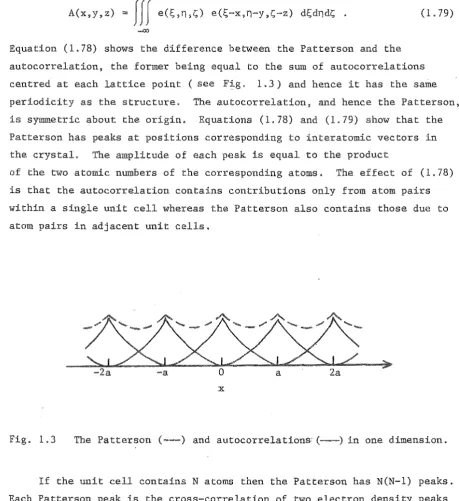
. (1. 79) -m

Equation (1.78) shows the difference between the Patterson and the autocorrelation, the former being equal to the sum of autocorrelations centred at each lattice point (see F:!-g. 1.3) and hence it has the same periodicity as the structure. The autocorrelation, and hence the Patterson, is symmetric about the origin. Equations (1,78) and (1.79) show that the Patterson has peaks at positions corresponding to interatomic vectors in the crystal, The amplitude of each peak is equal to the product

of the two atomic numbers of the corresponding atoms. The effect of (1.78) is that the autocorrelation contains contributions only from atom pairs

~.ithin a single unit cell whereas the Patterson also contains those due to

atom pairs in adjacent unit cells.

-2a -a 0 a 2a

.x

Fig. 1.3 The Patterson (---) and autocorrelations' (--) in one dimension.

If the unit cell contains N atoms then the Patterson has N(N-1) peaks. Each Patterson peak is the cross-correlation of two electron density peaks and so the width of a Patterson peak is the sum of the widths of the two corresponding electron density peaks. Hence the degree to which the

Patterson may be interpreted to give direct information on atomic positions depends critically on N. If N is very small (i.e. about 10 or so) the Patterson can often be unravelled directly, with the aid of independent chemical knowledge, to determine the atomic positions. However biological molecules may contain over 1000 atoms in the unit celL The Patterson then

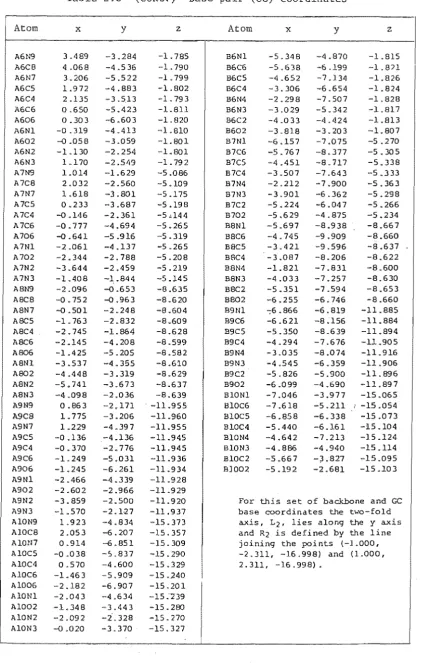
[image:30.549.47.507.64.566.2]

-20~

The main methods of phase determination, particularly for biological macromolecules, are chemical modification methods (Sherwood~ 1976, ch. 12). These all require investigation of the diffraction of at least two

crystals, one of which must contain a heavy atom (an atom with ===..:..;:.;;..::..:;;,;;;.,

a large atomic number). Isomorphous crystals have (nearly) identical crystallographic structure and very similar chemical constituents, The diffraction pattern of an isomorphous crystal in which a small number of atoms have been replaced by heavy atoms is measured and the Patterson is computed. Patterson peaks corresponding to interatomic vectors involving the atoms stand out and this usually allows the positions, of the heavy atoms to be determined. Let F and be the structure factors, at a point in reciprocal space, of the original and the isomorphous sample respectively. Then ::;

F

+

FH so that

1 Fr 12 "" IFI2

+

I

12

+

FF _H

*

+

F*F

H (L80)

where is the structure factor of the heavy atoms minus the structure factors of the atoms which they replaced. Equation (1.80) may be written

( 1.81)

where a and

S

are the phases of F and FR respectively. Now IFI and 1

are known from the diffraction patterns, and the p0sitions of the heavy atoms are found from the Patterson, allowing IFHI and

S

to be computed. Rence

(1.81) can be solved for a, the phase of the structure factor F. Unless the crystal has special symmetry properties, three isomorphous are

to obtain a unambiguously (Sherwood, 1976, ch. 12),

In some cases it is convenient to choose a heavy atom which has an absorption band close to the X-ray wavelength. The X-rays then suffer

(inelastic) scattering by the heavy atom, so the electron densi'ty behaves as a complex quantity and (1.75) is not satisfied. Information from anomalous scattering can assist in phase determination (Ramachandran and Srinivasan, 1970). Once the structure factor phases have been found, the electron density can be computed by Fourier

The atomic positions obtained as described in §1.7.3 are subject to inaccuracies due to errors in the measured structure intensities, errors in

finite number of measured structure factors and uncertainties in inferring the atomic positions from the electron density map. The effect of these errors on the structure can be minimised by refin~ment procedures.

Structure refinement normally proceeds in three stages. Fourier

refinement consists of computing structure factor phases from an estimate of the structure and using these, together with the observed magnitudes, to compute a new structure. The process is repeated until there is no significant change in the phases. This is similar to phase correction techniques used in other branches of image processing (see, for example, Fienup, 1978). Following this, a difference Fourier map is computed which is a Fourier synthesis using the difference between the observed and calculated structure amplitudes. Difference Fourier synthesis is used for the more precise location of atomic positions and identification of missing atoms. Finally the atomic positions are adjusted by minimising

(using least squares techniques) the crystallographic residual (or R-factor) R, given by

R

CI

_{IIF I -IF I I ) / I I F I}

m om c m mOm (1. 82)

where IF I and IF I are the mth structure amplitudes observed and o m c m

calculated respectively. At this stage the best possible estimate of the structure should have been obtained.

Often, particularly with biological macromolecules, high quality crystals cannot be obtained, which means that the diffraction data obtained is also of very low quality. In such cases, often the best that can be done is to propose a model for the structure and refine it using least squares refinement.

Structure determination using X-ray crystallography provides a good example of the essential role of

a priori

knowledge mentioned in §1.1. From chemical analysis the number and types of the atoms in the molecule and their electron density functions are known. Stereochemical

-22~

1.8 BATES' SOLUTION TO THE INVERSE SCATTERING PROBLEM

It was shown in §1.2 and §1,3 that, under appropriate conditions. E}l and acoustic scattering is accurately described by the Helmholtz equation (1. Solutions to the inverse scattering problem described so far have all been approximate as they assume that the scattering is weak. In this section a method proposed by Bates (1975) to exactly solve the inverse scattering problem for the Helmholtz equation is described. This seems to be the only published attempt to solve this problem in more than one spatial dimension. Exact solutions to the inverse scattering problem for the Schrodinger equation are discussed in §1.9.

The method is described for two space dimensions although it is easily extended to three dimensions by invoking spherical Bessel functions and spherical harmonics. A polar coordinate system (r,S) is introduced in S,

and Q is taken to be a circle of radius a circumscribing the scattering region so that

v

v(r,e)

r < a

=

1 r > a

The wavefunction is written as an angular Fourier series

00 tlJ(r,8,k) =

m=~

~ (r,k) exp(ime) m

} (1.83)

(1. 84)

Now ~ can be measured for r ~ a which allows the wave impedance vector Z at r a to be determined. The mth component of Z is defined by

Z (k) = ~ (r.k)/~'(r,k)

I

(1.85)

m m m r=a

where the prime denotes the derivative with respect to r, The inverse scattering problem is to determine V for r < a given Z. Firstly V and ~

are written as series of orthogonal functions satisfying the necessary boundary conditions at r = a. Since V = v(r,8) is equal to unity at r = a, it can be written as a Fourier-Bessel series (Watson, 1966, ch. 18)

co 00

n=~

A

np (g ria) exp(ine) np r < a (1. 86)

where J (0) is the cylindrical Bessel function of the first kind of order n n

and g is the pth zero of J so that

J (g ) "" 0 •

n np

An appropriate series for

W

which satisfies the impedance boundary condition (1.85) is the Dini series (Watson, 1966, ch. 18)

w

(r. 8, k)

m=..co

where the htm(k) are defined by

J (h_n )

=

(h_n la) Z J'(h_n ) • m X,m X,m m m x,m

(1.87)

(1. 88)

(1.89)

Note that the nQ,m can be determined, using (1.89), from the measurements Zm' (1.88) and the fact that the J satisfy Bessel's differential

m

(Watson, 1966, ch.

2), V

2

_W

_{can be written as}

00 00

b_{X,m n} (hn _X,m la)2 J _{m X,m} (hn ria) exp(im8) m=-oo

Substituting from (1.86), (1.88) and (1.90) into (1.22) and using the orthogonality of exp(im8) and J _{m X,m} (hn ria)

00 00

( [k2

I

I

(hQ,tm,/a)2] NQ,tm' oQ,Q,! 0mm'

m=-"" Q,=1

00

+

k2

I

A _{XQ, Q,'}

! ,

J

bQ,m 0

m'-m,p , ,m,m ,m -m,p

where Q,' > 0,

a

XQ"t' ,m,m' ,n,p(k) =

f

J (g _{n np} ria) J _{m X,m} (hn ria) J _m ,(h_{x, m} nf ,ria) r dr • o

a

NQ,m(k)

=

f

[J_m(hQ,mr/a)]2 r dr

o

and 6 is the Kronecker delta defined by ron

(1. 90)

(1.91)

(1. 92)

(1. 93)

6 =: 1

ron m := n

} (1.94)

o

m f:. n

The quantities defined by (1.92) and (1.93) can be computed from the measurements, and (1.91) can be treated as an infinite set of homogeneous,

inverse scattering determinant, must equal zero. The significant property of this determinant is that the only unknowns it contains are the A which

np characterise the inhomogeneity v, If measurements are made at a number, M

say, of values of k then

M

independent determinants are obtained, If

M

is

large then the determinants may be truncated to order M and

solved simultaneously for M values of the A thereby giving an estimate of np

V, However the determinant is very non-linear in the A and the practical np

numerical aspects of the method require further investigation,

At present there is no exact solution to the inverse scattering problem for the in more than one dimension. Although the method described above does not provide a closed form solution, it does go some of the way towards formulating such a solution,

1.9 THE GELFAND-LEVITAN TECHNIQUE

1.9.1

The (SE)

describes the (non-relativistic) quantum mechanical scattering of particles by the potential V = V(~). The wavefunction ~ characterises the particles

I

the wavenumber k is related to their energy. In this section the discussion is limited to the one dimensional form of (1.95).

(1. 96)

which applies to the scattering of plane waves by a plane stratified medium or, with slight modifications, by a circularly symmetric potential.

Equations of the form of (1.96) also describe EM scattering by a plane stratified plasma (Jordan and Ahn, 1979) and monochromatic EM plane,wave scattering by a plane stratified dielectric slab where the angle of incidence than the wavenumber) is the variable (Mittra

et aZ .. , 1972), Fourier (1.96) gives the time domain form

0/ )

'¥ ~ v'¥

o ,

(1.97)

The difference between the SE (1,96) or (1.97) and the Helmholtz equation (HE) (1,22) or (1.20) is that the function describing the inhomogeneity is multiplied by the wavefunction in the former rather than its second time derivative in the latter. This means that for the Schrodinger equation the propagation is dispersive and furthermore that the wavefront travels at the free space velocity c. Both of these

characteristics can be understood by examining the variation of propagation speed with wavenumber, The local propagation speed v inside the scattering region is equal to W/K where K is the local wavenumber. Reference to

(1.96) and (1.22) shows that

v == cO V/k2) for the SE

l

(1. 98)

==

cN

for the HE

J

Hence the SE is because v is a function of k, so that, even in a homogeneous medium. the shape of ~ with time as the different frequency components travel at different speeds. However the HE is non-dispersive because v is independent of k and so the wave shape is constant with time in a homogeneous medium. Examination of (1,98) shows, assuming V ~ 0. that v increases from

°

to c as Ikl varies from Q to 00,

so the wavefront of ~travels at the free space speed c. Hence the depth of penetration of ~ into the scattering region after a particular time is independent of the inhomogeneity V. However for the HE the wavefront travels at a c/v and so the depth of penetration is a function of the inhomogeneity

v.

The scattering of one-dimensional scalar waves may be described with the aid of the scattering matrix (or S-matrix). Consider. the scattering of monochromatic waves by a potential which vanishes at infinity, i.e. Vex) - 0 as x - ±oo. As Ixl approaches infinity, the medium approaches free space and the wavefunction satisfies the free space equation. so that

~ == A(k) exp(ikx)

+

B(k) exp(-ikx) as

} (1.99) C(k) exp(ikx) D(k) exp(-ikx) as

The scattering matrix S :: _{S(k) transforms the incoming waves into the}

outgoing waves:

( Al

=

s

[: 1

'" [ s 11 (k)

sIZ(k)

rl

·D ~ , _{s21 (k)} (k) lB

-26-Applying (1.100) to an incident wave from first the left (x _00) and then the right (x +00) shmvs that _{and s11 (and s12 and} are the

reflection and transmission coefficients respectively from the left (and right). The principle of reciprocity (Jones, 1964, §1.3.2) ensures that

(1.101)

and energy conservation requires that S be

_"

-I , ( 1.102)

where the superscript T denotes matrix transposition and I is the unit matrix. (S*)T is often called the Hermitian conjugate or adjoint of S. Carrying out the operations in (1.102) gives

} (1.103) and

1* s22 = 0 .

It can be shown (Kay, 1272) that (1.101) and (1.103), together with physically reasonable assumptions on the analytic properties of the s,.,

1J

imply that a knowledge of the reflection coefficient s21 (or s12) alone (but not the transmission coefficient alone) determines the remaining coefficients of the S-matrix. The significance of this is discussed in

§3.2. Inspection of (1.96) shows that for large k, the effect of the term

Vo/

is negligible so that

~ 1 and as (1.104)

If the HE (1.26) could be transformed into the SE (1.102) the solutions to both direct and inverse scattering problems formulated for the SE could be appfied to the HE. Such a transformation exists and has been called the

(Bates and Wall, 1976). Consider an inhomogeneity which is confined to the half-space x > 0 so that

v

1 x < 0

"'" v(x) x > 0

The Chandrasekhar transform is motivated by the first order WKB

solution (Heading, 1962), denoted here by ~ ~ ~WKB' to (1.26) which is

x

~

::::

V~

exp( -ik

f \)

(~) d~)

.

WKB _o (1. 106)

A

new coordinateu is' defined by

u x x < 0

} (1.107) x > 0

so

that

du

=

Vdx ( 1.108)

and a new wavefunction $ is defined by

(1. 109)

Equation (1.107) defines the electrical (or optical or acoustic) distance u into scattering region, and the wavefront travels with constant

c with respect to u. Substituting (1.108) and (1.109) into (1.26)

( l.1l0)

which is a SE where the "potentialll _q

q(u) is by

q

o

u < 0

(l.111) u > 0 .

Since

W

is identical to ~ in the free space region (where ~ is measured) then, if the inverse problem for the SE can be solved, q(u) can be

determined from the data. Then v(u) can be computed (in principle) by solving the non-linear differential equation (1.111) and

v

(x) determined using (1.108). The solution to the inverse problem for the SE is described in the following section.

It is worth noting that a similar SE to the HE has not been found.

1.9.3

The Gelfand~Levitan (GL) technique is a method for solving exactly the

inverse scattering problem for the one-dimensional SE. It has received a considerable amount of attention in the more theoretical literature on inverse scattering; probably because it provides an explicit mathematical solut.ion t.o this particular problem, However the method is not

amenable to numerical computation and so there has been very little reported on the processing of real scattering data. The method itself is an outgrowth of the work of two mathematicians, Gelfand and Levitan (1951), on a type of differential equation. Their work has been extended and applied to a number of inverse scattering problems. The technique has also been widely used in the solution of non-linear differential equations (Sabatier, 1978).

Most reported derivations of the GL equation use spectral techniques (see, for example, Newton, 1966, §20.2), however these are not easily understood by non~mathematicians unfamiliar with spectral theory. For this reason a more physically motivated derivation in the time domain

us causality (following Kay, 1960) is given here. Almost. all derivations of the GL equation in the literature gloss over the details (some of which are quite intricate) so I consider it useful to present a fairly detailed treatment here. For convenience, subscripts are used in this section to denote partial derivatives,

Consider the by an inhomogeneous half space x > 0 (see

1.4 (a) described by the SE (1.96) so that the potential V satisfies

Vex) =:: 0 x < 0 • (1.112)

The reflection coefficient from the left, s21(k), which is denoted here by r(k). is measured as a function of k at some point in the free' space region x < 0, Let R(x+ct) be the reflected field in the region x < 0 due to the incident field 8(x~ct) so that the total field in this region is given by

lJ!(x,t) "" o(x ct) + R(x+ct) x < 0 (1.113)

Since no reflected field appears before the incident field strikes the scattering region

at

x 0, causality implies that

• 1.4

x (a)

---

__ .,- - cfl(x, t)

x

(b)

One-dimensional scat by a potential. (a) The potential V.

(b) The form of the wavefunctions ¢ and

'¥ at time t.

The impulse response R(T) is equal to the FT of r(k), i.e.

R(T) ::::

J

r(k) exp( -i21TkT) dk . (1.l15)

So R(T) may be measured directly or computed from a measurement of r(k).

A free space field cfl = cfl(x,t) is defined .;;;.,;:..:::-~;.;;:;;....= x by

¢(x,t) == o(x-ct) +R(x+ct)

, 'it

x (1.116)

and hence satisfies the free space equation

_{- - - - -}

all x

= 0

'it

x (1.117)

Hence ¢ is an extension of '¥ for x < 0 by 0.l13) into the region x > 0 assuming that all of space is free (V

=

0).

An essential step is to assume that the solution '¥ to (1.97) is given by a linear transformation of the solution ¢ of the free space equation