IN NATURAL AND AGRICULTURAL HABITATS AND AN ANALYSIS OF PREDATOR COMMUNITIES USING STABLE ISOTOPES OF CARBON AND NITROGEN
by
Kathlyn Jean McVey
A thesis
submitted in partial fulfillment of the requirements for the degree of Master of Science in Raptor Biology
Boise State University
May 2011
DEFENSE COMMITTEE AND FINAL READING APPROVALS
of the thesis submitted by
Kathlyn Jean McVey
Thesis Title: Trophic Ecology of Burrowing Owls in Natural and Agricultural Habitats and an Analysis of Predator Communities using Stable Isotopes of Carbon and Nitrogen
Date of Final Oral Examination: 10 March 2011
The following individuals read and discussed the thesis submitted by student Kathlyn Jean McVey, and they evaluated her presentation and response to questions during the final oral examination. They found that the student passed the final oral examination.
James R. Belthoff, Ph.D. Chair, Supervisory Committee Peter Koetsier, Ph.D. Member, Supervisory Committee Mark R. Fuller, Ph.D. Member, Supervisory Committee
The final reading approval of the thesis was granted by James R. Belthoff, Ph.D., Chair of the Supervisory Committee. The thesis was approved for the Graduate College by John R. Pelton, Ph.D., Dean of the Graduate College.
iv
I dedicate this thesis to my wonderful family and friends.
Thank you for all your support, kind words, and hours spent on the phone.
v
I would first like to thank the members of my family, both new and old, who provided me with support every step of the way during this long journey. I truly could not have completed my research and thesis without them. I wish to thank my advisor Dr.
James Belthoff for his guidance, patience, and especially flexibility in allowing me to finish my thesis from afar. This thesis would not be complete without the thoughtful input and advice from my committee members Dr. Mark Fuller and Dr. Peter Koetsier whom I thank. I thank my fellow burrowing owl researchers, Matt Stuber and Justin Welty, as their help and camaraderie in the field was invaluable. And to the many other students, volunteers, and friends who offered their assistance in the field, classroom, or at happy hour, I appreciate your support. I would like to thank the Raptor Research Center for providing me a work space and use of vehicles for my thesis research. Thank you to the various sources who helped to fund my research including the USDA Cooperative State Research, Education, and Extension Service; Boise State University; and the Raptor Research Center. Finally, I thank the National Science Foundation GK-12 Fellowship program; the Foothills Learning Center in Boise, Idaho; AmeriCorps; and the US Fish and Wildlife Service for presenting me with opportunities and experiences that have helped shaped my thesis and my life.
vi
Stable isotopes of carbon and nitrogen can provide powerful tools for estimating the trophic positions of animals and determining the source or the primary producer of a food web. I used stable isotopes analysis of carbon (δ13C) and nitrogen (δ15N) to
investigate the trophic position of burrowing owls (Athene cunicularia) in agricultural and natural habitats and trophic relationships of a community of vertebrate predators in the Morley Nelson Snake River Birds of Prey National Conservation Area (NCA), located in southern Idaho.
Burrowing owl populations have declined across much of North America owing to loss of habitat. However, burrowing owls show affinity for nesting near agriculture in some portions of their range, including s. Idaho. I used analysis of 13C and 15N to
investigate burrowing owl food habits and trophic relationships in agricultural and natural habitats in the NCA. δ13C did not differ between natural and agricultural habitats and indicated carbon sources in burrowing owl diet contained primarily C3 plants.
Conversely, δ13C differed between nestling and adult owls, which may indicate that adults provisioned nestlings with a different diet than they consumed. Burrowing owl δ15N values depended on both habitat (i.e., natural or agricultural) and group (i.e., samples from 20 day old juveniles, 30 day old juveniles, adult females or adult males), although owls nesting in natural habitat generally had higher δ15N values than owls nesting in agricultural habitat. Owls in natural habitat potentially fed on more kangaroo rats (Dipodomys ordii), scorpions (Hadrurus spadix) and spiders (Infraorder
Mygalomorphae) and fewer montane voles (Microtus montanus) and crickets (Gryllus spp.), which may help explain elevated δ15N values for owls nesting in natural habitat.
My results corroborated Moulton et al. (2005, 2006), who used traditional food habits analysis and found that burrowing owls nesting in natural and agricultural habitats feed on different prey species in each habitat. As adults in natural areas had higher δ15N values, this may be further evidence that adult owls consumed different prey than they used to provision nestlings. Food webs, of which burrowing owls are a part, for both natural and agricultural habitats were similar despite the introduction of irrigated agriculture into a naturally arid landscape.
I also examined trophic relationships of a community of vertebrate predators in the same area. The NCA has a rich diversity of predators, including sixteen raptor species and an array of mammalian predators. It presents a unique opportunity to examine trophic ecology of predators that may use the same prey resources. I compared my results from analysis of 13C and 15N with results from traditional food habit study methods from Marti et al. (1993). I collected 272 samples from 14 species of vertebrate predator. Predators had a relatively narrow range of δ15N with only 2‰ separating the majority of the species; therefore, the vertebrate predators that I examined occupied a similar trophic position. The food web in the NCA is based on a combination of C3 and C4 plants and illustrates that a mixture of plant species is supporting a community structure of herbivores, omnivores, and predators, rather than a particular species of shrub, forbs, grass, or crop plant. My findings were consistent with the results from Marti et al. (1993), who found, when prey were identified to the class level, mean dietary overlap among vertebrate predators was 82%. As in Marti et al. (1993), results based on
vii
viii
while two species (coyotes, Canis latrans and great horned owls, Bubo virginianus)were sufficiently dissimilar and were excluded from other groups. By pairing stable isotope technology with traditional food habit study methods, my study provides a more complete view of trophic relationships among vertebrate predators.
ix
TABLE OF CONTENTS
ABSTRACT ... vi
LIST OF TABLES ... xii
LIST OF FIGURES ... xiii
CHAPTER 1: STABLE ISOTOPES OF CARBON AND NITROGEN AND THEIR USE IN UNDERSTANDING TROPHIC ECOLOGY ... 1
What Are Stable Isotopes? ... 1
Nitrogen ... 2
Carbon ... 4
Samples for Isotope Analysis ... 5
How to Use Stable Isotopes ... 6
Overview of Chapters 2 and 3 ... 9
Literature Cited ... 15
CHAPTER 2: A COMPARISON OF TROPHIC RELATIONSHIPS OF BURROWING OWLS IN AGRICULTURAL AND NATURAL HABITATS USING STABLE ISOTOPIC ANALYSIS ... 19
Abstract ... 19
Introduction ... 20
Objective 1: Compare Burrowing Owl Food Habits Between Habitats and Among Groups ... 25
Objective 2: Establish Food Webs for Agricultural and Natural Habitats ... 26
Study Species ... 26
x
Methods ... 29
Burrowing Owl Sample Collection and Nest Monitoring ... 29
Plants ... 31
Invertebrates ... 31
Vertebrate Samples Collected from Burrowing Owl Nests Sites ... 32
Vertebrate Samples Collected from Roadway Surveys ... 32
Stable Isotopes Analysis ... 32
Statistical Analysis ... 33
Results ... 34
Food Habits: Differences Between Habitats and Among Burrowing Owl Groups ... 34
Food Webs for Agricultural and Natural Habitats ... 35
Discussion ... 38
Food Habits: Differences Between Habitats and Among Burrowing Owls ... 40
Establish Food Webs Using Stable Isotopes Analysis ... 44
Conclusions ... 50
Literature Cited ... 57
CHAPTER 3: TROPHIC RELATIONSHIPS AMONG VERTEBRATE PREDATORS IN THE MORLEY NELSON SNAKE RIVER BIRDS OF PREY NATIONAL CONSERVATION AREA ... 65
Introduction ... 65
Methods ... 68
Stable Isotopes Analysis ... 69
xi
Results and Discussion ... 70
Summary and Conclusions ... 76
Literature Cited ... 82
APPENDIX ... 86 List of species and δ13C and δ15N values from groups of species found
in Figure 3.2
xii
LIST OF TABLES
Table 2.1 Species sampled in natural and agricultural habitats for stable isotopes analysis. Mean ± SE are presented for each isotope within each habitat. Group headings or species are listed in Figure 2.4 are in gray, and species below each group heading
constitutes group members. ... 55
xiii
LIST OF FIGURES
Figure 1.1 An example of trophic relationships among plants and categories of animals as illustrated by stable isotopes of carbon and nitrogen.
Graph is modified from Bemis et al. (2003). ... 12 Figure 1.2 Carbon isotopes distributed typical of plants species using C3
or C4 photosynthetic pathways. Graph is modified from
O‟Leary‟s (1988). ... 13 Figure 1.3. Conventional display of δ15N and δ13C in a dual isotope plot. This
example, from Inger and Bearhop (2008), indicates how consumers and prey can differ in δ15N and how carbon sources can differ from terrestrial to marine inputs. ... 14 Figure 2.1. Burrowing owl diet delineated by habitat (revised from Moulton
et al. 2005). ... 51 Figure 2.2. Burrowing owl δ13Carbon values (mean SE). Values not sharing
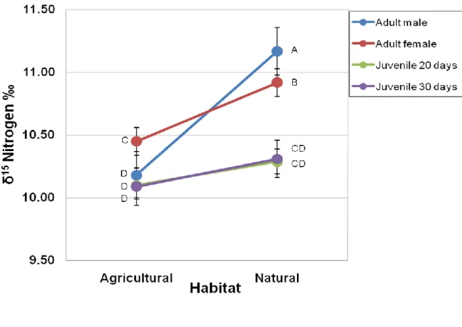
the same letter differ significantly. ... 52 Figure 2.3. Burrowing owl δ15Nitrogen values (mean ± SE). Values not sharing
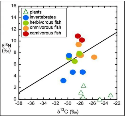
The same letter are significantly different. ... 53 Figure 2.4. δ15Nitrogen and δ13Carbon isotope values for the presumptive food
web of burrowing owls in natural and agricultural habitats.
Mean ± SE are listed for each group or species (see text). Triangles represent samples from natural habitat, and squares represent
samples from agricultural habitat. Primary Producers - green circles;
Primary Consumers - red circle; Secondary Consumers - blue circle;
Higher-level consumers - black circle. ... 54
xiv
identified to species/genus level (from Marti et al. 1993:12). Avian predator name abbreviations correspond to the American
Ornithologists‟ Union abbreviations as follows: NOHA = northern harrier, RTHA = red-tailed hawk, FEHA = ferruginous hawk, GOEA = golden eagle, AMKE = American kestrel, PRFA = prairie falcon, BANO = barn owl, WESO = western screech-owl,
GHOW = great horned owl, BUOW = burrowing owl, LEOW = long-eared owl, NSWO = northern saw-whet owl, and CORA = common raven. Abbreviations for mammals and reptiles are based on scientific names: CALA = coyote, TATA = badger, PIME = gopher snake, and CRVI = western rattlesnake. See text for
scientific names. ... 79 Figure 3.2. Mean (± SE) δ15Nitrogen and δ13Carbon for species of vertebrate
Predator in the Morley Nelson Snake River Bird of Prey National Conservation Area. Number of samples for each group or species is in parentheses. Mean (± SE) δ15N and δ13Cvalues for groups of potential prey species are shown in grey (See Chapter 2 for methods related to prey species isotopes and Appendix for a list of species
within each group of prey species). ... 80
Figure 3.3. Hierarchical clustering (Ward‟s method, dendrogram distance scale) of δ15Nitrogen and δ13Carbon results for the vertebrate predator community in the Morley Nelson Snake River Bird of Prey National Conservation Area. Red lines separate the resulting clusters. Avian predator name abbreviations correspond to the American
Ornithologists‟ Union abbreviations as follows: FEHA = ferruginous hawk, RTHA = red-tailed hawk, AMKE = American kestrel,
PRFA = prairie falcon, WESO = western screech-owl, GHOW = great horned owl, BUOW = burrowing owl, SEOW = short-eared owl, NSWO = northern saw-whet owl, and CORA = common raven.
Abbreviations for mammals and reptiles are based on scientific names: CALA = coyote, TATA = badger, MUFR = long-tailed
weasel, and PIME = gopher snake. See text for scientific names. ... 81
CHAPTER 1: STABLE ISOTOPES OF CARBON AND NITROGEN AND THEIR USE IN UNDERSTANDING TROPHIC ECOLOGY Since their first uses in earth science research, applications of stable isotopes analysis in other disciplines, particularly ecology, have rapidly expanded. Stable isotopes of carbon and nitrogen can provide powerful tools for estimating the trophic positions of consumers in a food web and the carbon flow to such consumers (Kelly 2000, Post 2002, Fry 2006, Inger and Bearhop 2008). Furthermore, the ongoing advances in modeling techniques and laboratory approaches, the incorporation of additional isotopes (sulfur, oxygen, and hydrogen), and the relative decrease in cost of analysis have combined to greatly increase the number of studies using this technique. Stable isotopes analyses have been used extensively to investigate aquatic food webs, but their use in understanding terrestrial ecosystems is more recent. This chapter of my thesis provides an overview of how nitrogen and carbon stable isotopes are used in elucidating trophic ecology, which will facilitate understanding of the field studies that I describe in Chapters 2 and 3.
What Are Stable Isotopes?
Isotopes are chemical elements differing in the number of neutrons. Stable isotopes, unlike radiogenic isotopes, do not decay over time. Stable isotopes generally have one more neutron than a common form of the element and, thus, are heavier.
Naturally occurring stable isotopes are found for biologically important elements, e.g., carbon, hydrogen, nitrogen, oxygen, and sulfur (Fry 2006, Inger and Bearhop 2008). The stable isotopes useful in trophic ecology are found in very low abundances. For instance,
of all the carbon in the world, 98.9% is 12C (i.e., the common form), and only 1.1% is 13C (Rundel et al. 1989). These differences in relative abundance of isotopes can be
measured by mass spectrometry in the laboratory. Continuous-flow isotope-ratio mass spectrometers (CFIRMS) allow multiple isotopes to be analyzed simultaneously, which has greatly reduced the cost of analysis and makes this technique more practical (Inger and Bearhop 2008).
Stable isotope natural abundances are expressed as a delta () in parts per mill (‰), where denotes the difference between a sample and an international standard.
International standards for carbon, nitrogen, and hydrogen are Pee Dee Belemnite, atmospheric nitrogen (air), and Vienna Standard Mean Ocean Water (VSMOW), respectively. The expression for an isotope sample is:
X = [ (RSAMPLE / RSTANDARD) – 1 ] * 1000
where X is the element of interest, RSAMPLE = the ratio of heavy to light isotopes in the sample, and RSTANDARD = the ratio of the heavy to light isotopes in the standard (Kelly 2000, Fry 2006, Inger and Bearhop 2008). Lighter isotopes are more quickly broken down than heavier isotopes and, as a result, many chemical and physical processes lead to isotopic fractionation. Carbon (13C/12C) and nitrogen (15N/14N) are the two isotopes most frequently used in food habits analysis. Their analysis provides results that are useful in determining trophic structure and food webs for a wide variety of organisms and habitats.
Nitrogen
Nitrogen (15/14N) shows predictable bioaccumulation of 2 - 4‰ per step upward in the food chain; thus, it is key to understanding trophic position of a species (Minagawa and Wada 1984, Post 2002). Bioaccumulation occurs as a result of differential
fractionation between the heavy and light isotopes. 14N is more easily digested and excreted in waste products, whereas 15N becomes incorporated into the tissues of the consumer (DeNiro and Epstein 1981, Fry 2006). Thus, a consumer‟s tissues tend to be enriched in15N relative to the plants and animals in its diet. For example, if primary producers (plants) have a δ15N value of 3‰, then one would expect primary consumers (herbivores) to have a δ15N value of around 7‰. Secondary consumers (carnivores) would have a δ15N value of around 11‰ (Figure 1.1, Bemis et al. 2003).
δ15N bioaccumulation or isotopic enrichment factors are known for a variety of animals at many levels of presumptive food chains. Average fractionation of 3.4‰ is a robust and widely applicable assumption of the expected isotopic difference between animals of different trophic levels when applied to entire food webs with multiple pathways (Post 2002). However, choosing a specific enrichment factor between 2 and 4‰ will not dramatically affect the conclusions drawn from comparisons among
organisms in the same food web. Comparing δ15N values across food webs and habitats is generally appropriate when baseline measures of plants, litter, or soil are available to make inter-site comparisons (Nakagawa et al. 2007). Overall, analysis of
bioaccumulation of δ15N values allows one to assign trophic level and relative position in the food chain to a species (Fry 2006). For example, Hyodo et al. (2010) used analysis of nitrogen and carbon stable isotopes to examine trophic relationships of various animal consumers within a tropical rain forest in Malaysia. They found detritovores, omnivores, herbivores, and carnivores had distinct isotope values, and that herbivores derive most of their carbon from the forest canopy layer. O‟Grady et al. (2010) studied several species of ants in a temperate limestone grassland. Using 15N, they were able to tease apart
trophic structure of ant species and found δ 15N values for adult Lasius flavus were higher than expected, which suggested a more predatory diet than was implied in the literature.
Thus, stable isotopes analysis led to new understanding of diets for coexisting species of ants.
Carbon
13C shows less predictable bioaccumulation of between 0.7 - 1.3‰ (O‟Leary 1988) and is more commonly used to determine the primary energy or source of carbon input at the base of the food web. Plant species use three different photosynthetic pathways: C3, C4, and CAM. C3 and C4 photosynthesis are the most common, and each pathway presents itself with a distinct 13C range (Figure 1.2). The plants that use C3
photosynthesis, mainly forbs, are characteristically more depleted in 13C, with an average of -28‰. Grasses, such as corn (Zea mays) and cheatgrass (Bromus tectorum), are C4 plants and are comparatively enriched in 13C, with an average of -14‰ (Figure 1.2, O‟Leary 1988, Rundel et al. 1989). There is very little overlap in the 13C range for C3 and C4 plants; therefore, it is often possible to determine what types of plants are at the base of a food chain of interest (Figure 1.2, DeNiro and Epstein 1978, O‟Leary 1988).
Analysis of carbon isotopes can also determine from what habitat type an animal has been feeding, either marine or terrestrial (Figure 1.3, Hobson 1990, Inger and Bearhop 2008), or which types of plants were the most important to sustaining a food web (Wolf and Martínez del Rio 2003). 13C and 15N are often used in combination to examine food habits of an animal and can elucidate the primary energy source and species‟ relative trophic position for a food web.
Samples for Isotope Analysis
As plant and animal tissues have specific turnover rates, stable isotope values reflect the diet for specific periods of time depending on which tissue(s) are analyzed.
Hobson and Clark (1992a) found that isotope values in whole blood of captive Japanese quail (Coturnix japonica) have a half-life of 11.4 days, so samples of isotopes from blood reflect recent diet. Isotopes in muscle have a slightly longer half-life of 12.4 days. Liver tissue has very short isotopic half-lives of 2.6 days, while bone collagen has a long half- life of about 173.3 days (Hobson and Clark 1992a). Miller et al. (2008) found that for deer mice (Peromyscus maniculatus) in a laboratory setting, nitrogen isotopes have a half-life of 19.8 days in whole blood and 24.8 days for muscle. However, Nagy (1987) suggested care be taken when extrapolating laboratory derived enrichment factors such as those just mentioned to wild populations. He found wild bird metabolic rates are often higher than the basal metabolic rates of caged animals.
Stable isotope analysis of fur, hair, and feathers can yield longer-term dietary information. Isotopes values from feathers in birds reflect the diet from when the feather was growing, as after a feather has emerged from the blood shaft, it is isotopically inert.
The same is true with fur and hair in mammals. Therefore, it is important to know at what time and geographic location the fur or feather grew. For some bird species, it may be more than one year to complete one molt cycle, e.g., barn owls (Tyto alba) have a molt pattern of longer than two years. Therefore, they are a species where sampling two different primary feathers will yield two years of stable isotope values (Cramp 1985, Taylor 1994). When using stable isotopes analysis, it is important to define what time period one is trying to study and choose sample type according to that time frame.
Rates of assimilation or trophic enrichment values may differ based on sample type as well. Miller et al. (2008) found mean enrichment values for deer mice for blood and muscle to be -0.2‰ and -0.7‰ for carbon and 2.3‰ and 2.5‰ for nitrogen,
respectively (no SE was reported). Hobson and Clark (1992b) studied peregrine falcon (Falco peregrines) blood and feather samples and found trophic enrichment values to be 0.2 ± 0.01‰ and 2.1 ± 0.08‰ for carbon and 3.3 ± 0.4‰ and 2.7 ± 0.5‰ for nitrogen, respectively. Tissues such as blood, muscle, and feathers are synthesized at different rates and potentially from different dietary components, as muscle and feathers are composed of protein, and blood is a mixture of sugars, protein, and other solutes. This makes it difficult to draw direct comparisons of isotope values across different tissues, as trophic enrichment factors can vary by tissue type (Inger and Bearhop 2008). However, Croxall et al. (1999) found isotope values derived from blood samples have an advantage of allowing comparisons among birds and mammals more easily than comparing isotope values derived from fur and feathers. Hobson and Clark (1992b) also found that for birds whose diet is animal protein, nitrogen fractionation values do not differ between young and adult birds.
How to Use Stable Isotopes
Mixing models based on stable isotopes analysis can be employed in some cases to further elucidate a species‟ position within an ecosystem and estimate percent of important prey species in a consumer‟s diet. However, complex systems with a diversity of species and sample types make it difficult to apply a mixing model (Kelly 2000, Post 2002, Fry 2006, Inger and Bearhop 2008). Many mixing models have specific
requirements that can be hard to fulfill in a natural study. In addition to adequate
sampling of prey species (O‟Grady et al. 2010) and temporal matching of diet and prey, mixing models usually require a low number of isotopically distinct nutrient sources and information on the isotopic heterogeneity of a species‟ diet or habitat (Inger and Bearhop 2008). Another complication of mixing models is that the output of these models
corresponds to a set of possible solutions, rather than the real solution (Inger and Bearhop 2008).
Plots of δ13C and δ15N values and cluster diagrams are common methods to portray the results of food habits studies and trophic analyses based on isotopes. Carbon and nitrogen stable isotope values are traditionally displayed in a dual isotope plot with δ13C on the x-axis and δ15N on the y-axis (Figure 1.1, Figure 1.3). Isotope plots
demonstrate trophic enrichment between food source and consumer and may elucidate differences in carbon source for species of interest (Figure 1.3). Additionally, cluster analysis of isotope values may be used to group species with similar dietary habits (Davenport and Bax 2002, Roth et al. 2007). Roth et al. (2007) used cluster analysis and found snowshoe hares (Lepus americanus), one of the most common prey items of Canada lynx (Lynx canadensis), were isotopically distinct from all other prey species.
Some studies use an index or reference species with well-known dietary habits as a baseline to better interpret isotope values for species with less well-known food habits (see Herrera et al. 2003).
Perhaps the best approach to understanding diet is to combine stable isotopes analysis with traditional food habit study methods. Traditional approaches to
understanding diet include analyses of stomach contents, fecal materials, or prey remains;
direct observation; and, in some cases, examination of regurgitated pellets where partially
or undigested materials can be identified. While these methods can provide accurate taxonomic information about an animal‟s diet, they may not work well for animals that consume small prey items or forage a great distance from land. Isotope studies can offer novel insights into trophic relationships using a tool that is independent of traditional techniques (Evans Ogden et al. 2005).
Studying food habits using stable isotopes analysis may have some advantages over traditional food habits study methods. Most prominently, isotope samples are a reflection of not only what an animal eats, but what is assimilated and incorporated into the consumer. As animals „are what they eat,‟ stable isotope values in a consumer‟s tissues reflect their diet, and consequently allow one to understand a consumer‟s food habits and trophic level within a habitat. Additionally, some samples for isotopes analysis such as feathers and fur can be collected non-invasively as they are shed throughout the year, while other sample types such as blood, toenail clippings, and muscle can be collected non-lethally. Samples collected during one trip to a nest or roost site can simultaneously yield information about an animal‟s recent and long-term diet, while only disturbing the animal once. Finally, while isotopes are weaker at providing taxonomic detail of diet and cannot typically distinguish diet contributions among
trophically similar prey, they can provide better estimates of the role that soft-bodied prey items play in an animal‟s diet when compared to traditional methods. For instance, stable isotope analysis revealed differences in trophic level between seabirds living on two islands was caused by greater amounts of soft-bodied invertebrate prey consumed by birds on one of the two islands (Hobson et al. 2002).
Stable isotopes analysis can also be used to define trophic structure within an ecosystem and detect changes in diet that may occur across a group of individuals.
Cherel et al. (2007) examined resource partitioning within a guild of air-breathing diving predators and demonstrated that guild structure did not change between summer and winter. Yi et al. (2006) used stable isotopes to categorize animals into trophic groups and found seasonal differences within omnivorous bird species occupying a Tibetan Plateau.
Davenport and Bax (2002) investigated a marine ecosystem off the coast of Australia.
They used cluster analysis of isotope values from fish species and produced groupings of trophic relationships that were supported by stomach contents analysis. Stable isotopes can also be a useful tool to study how alteration of natural landscapes can impact a species‟ food habits. Using stable isotopes analysis, Evans Ogden (2005) found that wintering dunlins (Calidris alpine pacifica) forage extensively in agricultural habitat.
Overview of Chapters 2 and 3
In Chapter 2 of this thesis, I report the results of my use of analyses of δ13C and δ15N to investigate western burrowing owl (Athene cunicularia hypugaea) food habits and trophic relationships in agricultural and natural habitats in the Morley Nelson Snake River Birds of Prey National Conservation Area (NCA) in southern Idaho. Burrowing owl populations have declined across much of North America (Haug et al. 1993, Gervais and Anthony 2003). However, they show affinity for nesting near agriculture in some portions of their range (Rich 1986, Leptich 1994, DeSante et al. 2004, Conway et al.
2006, Moulton et al. 2006, Restani et al. 2008). Using analysis of δ13C and δ15N, I found the food webs, of which burrowing owls are a part, in both natural and agricultural habitats were similar despite the introduction of irrigated agriculture into a naturally arid
landscape. For burrowing owls, carbon isotopes did not differ between natural and agricultural habitats and indicated carbon sources in burrowing owl diet contained
primarily C3 plants. However, δ13C differed between nestling and adult owls, which may signify that adults provisioned nestlings with a different diet than they consumed.
Burrowing owl δ15N values depended on both habitat (i.e., natural or agricultural) and group (i.e., samples from 20 day old juveniles, 30 day old juveniles, adult females or adult males), although owls nesting in natural habitat generally had higher δ15N values than owls nesting in agricultural habitat. Owls in natural habitat potentially fed on more kangaroo rats (Dipodomys ordii), scorpions (Hadrurus spadix), and spiders (Infraorder Mygalomorphae) and fewer montane voles (Microtus montanus) and crickets (Gryllus spp.), which may help explain elevated δ15N values for natural habitat. My results corroborated Moulton et al. (2005, 2006), who found using traditional food habits analysis that burrowing owl nesting in natural and agricultural habitats feed on different prey species in each habitat. As adults in natural areas had higher δ15N, this may be further evidence that adult owls consumed different prey than they used to provision nestlings.
In Chapter 3 of this thesis, I examined trophic relationships of a community of vertebrate predators in s. Idaho. While the NCA has an array of mammalian predators, the diversity of avian predators and density of breeding raptors is unparalleled within North America. Sixteen raptor species regularly breed within the NCA and eight other species use the area while migration or wintering. This rich diversity of species presents a unique opportunity to examine relationships among a variety of vertebrate predators that may use the same prey resources. I compared my results from isotope analysis of
carbon (13C) and nitrogen (15N) with results from traditional food habit study methods in Marti et al. (1993). I collected samples from 14 species of vertebrate predator including five species of owl, two hawks, two falcons, three mammals, one reptile, and one additional bird species. Predators had a relatively narrow range of mean δ15N with only 2‰ separating 13 of the 14 predators; therefore, the species of vertebrate predator that I examined occupied similar trophic positions. My findings were consistent with the results from Marti et al. (1993), who found, when prey were identified to the class level, mean dietary overlap among vertebrate predators was 82%. Pairing stable isotope technology with traditional food habit study methods may provide a more complete view of trophic relationships among vertebrate predators.
Figure 1.1. An example of trophic relationships among plants and categories of animals as illustrated by stable isotopes of carbon and nitrogen. Graph is modified from Bemis et al. (2003).
Figure 1.2. Carbon isotope distribution typical of plants species using C3 or C4 photosynthetic pathways. Graph is modified from O‟Leary (1988).
Figure 1.3. Conventional display of δ15N and δ13C in a dual isotope plot. This example, from Inger and Bearhop (2008), illustrates how consumers and prey can differ in δ15N and how carbon sources can differ from terrestrial to marine inputs.
Literature Cited
Bemis, B.E., C. Kendall, S.D. Wankel, T. Lange, and D.P. Krabbenhoft. 2003. Isotopic evidence for spatial and temporal changes in Everglades food web structure.
Poster presented at Greater Everglades Ecosystem Restoration Conference. Palm Harbor, Florida.
Cherel, Y., K.A. Hobson, C. Guinet, and C. Vanpe. 2007. Stable isotopes document seasonal changes in trophic niches and winter foraging individual specialization in diving predators from the Southern Ocean. Journal of Animal Ecology 76:826- 836.
Conway, C.J., V. Garcia, M.D. Smith, L.A. Ellis, and J.L. Whitney. 2006. Comparative demography of burrowing owls in agricultural and urban landscapes in
southeastern Washington. Journal of Field Ornithology 77:280-290.
Cramp, S. 1985. The Birds of the Western Palearctic. Vol. 4. Oxford University Press, Oxford.
Croxall, J.P., K. Reid, and P.A. Prince. 1999. Diet, provisioning and productivity responses of marine predators to differences in availability of Antarctic krill.
Marine Ecology-Progress Series 177:115-131.
Davenport, S.R. and N.J. Bax. 2002. A trophic study of a marine ecosystem off southeastern Australia using stable isotopes of carbon and nitrogen. Canadian Journal of Fisheries and Aquatic Sciences 59:514-530.
DeNiro, M.J. and S. Epstein. 1978. Influence of diet on the distribution of carbon isotopes in animals. Geochimica et Cosmochimica Acta 42:495-506.
DeNiro, M.J. and S. Epstein. 1981. Influence of diet on the distribution of nitrogen isotopes in animals. Geochimica et Cosmochimica Acta 45:341-351.
DeSante, D.F., E.D. Ruhlen, and D.K. Rosenberg. 2004. Density and abundance of burrowing owls in the agricultural matrix of the Imperial Valley, California.
Studies in Avian Biology 27:116-119.
Evans Ogden, L.J., K.A. Hobson, D.B. Lank, and S. Bittman. 2005. Stable isotope analysis reveals that agricultural habitat provides an important dietary component for nonbreeding Dunlin. Avian Conservation and Ecology 1.3.
http://www.ace-eco.org/vol1/iss1/art3/.
Fry, B. 2006. Stable Isotope Ecology. Springer, New York.
Gervais, J.A. and R.G. Anthony. 2003. Chronic organochlorine contaminants,
environmental variability, and the demographics of a burrowing owl population.
Ecological Applications 13:1250-1262.
Haug, E.A., B.A. Millsap, and M.S. Martell. 1993. Burrowing Owl (Athene cunicularia), The Birds of North America Online (A. Poole, ed.). Ithaca: Cornell Lab of
Ornithology; Retrieved from the Birds of North America Online:
http://bna.birds.cornell.edu/bna/species/061doi:10.2173/bna.61.
Herrera, L.G., K.A. Hobson, M. Rodríguez, and P. Hernandez. 2003. Trophic partitioning in tropical rain forest birds: insights from stable isotope analysis. Oecologia 136:439-444.
Hobson, K.A. 1990. Stable isotope analysis of marbled murrelets: evidence for freshwater feeding and determination of trophic level. Condor 92:897-903.
Hobson, K.A. and R.G. Clark. 1992a. Assessing avian diets using stable isotopes I:
turnover of 13C in tissues. Condor 94:181-188.
Hobson, K.A. and R.G. Clark. 1992b. Assessing avian diets using stable isotopes II:
factors influencing diet-tissue fractionation. Condor 94:189-197.
Hobson, K.A., G. Gilchrist, and K. Falk. 2002. Isotopic investigations of seabirds of the North Water Polynya: contrasting trophic relationships between the eastern and western sectors. Condor 104:1-11.
Hyodo, F., T. Matsumoto, Y. Takematsu, T. Kamoi, D. Fukuda, M. Nakagawa, and T.
Itioka. 2010. The structure of a food web in a tropical rain forest in Malaysia based on carbon and nitrogen stable isotope ratios. Journal of Tropical Ecology 26:205-214.
Inger, R. and S. Bearhop. 2008. Applications of stable isotope analyses to avian ecology.
Ibis 150:447-461.
Kelly, J. 2000. Stable isotopes of carbon and nitrogen in the study of avian and mammalian trophic ecology. Canadian Journal of Zoology 78:1-27.
Leptich, D.J. 1994. Agricultural development and its influence on raptors in southern Idaho. Northwest Science 68:167-171.
Marti, C.D., K. Steenhof, M.N. Kochert, and J.S. Marks. 1993. Community trophic structure: the roles of diet, body size, and activity time in vertebrate
predators. Oikos 67:6-18.
Miller, J.F., J.S. Millar, and F.J. Longstaffe. 2008. Carbon- and nitrogen-isotope tissue- diet discrimination and turnover rates in deer mice, Peromyscus maniculatus.
Canadian Journal of Zoology 86:685-691.
Minagawa, M. and E. Wada. 1984. Stepwise enrichment of 15N along food chains: further evidence and the relation between 15N and animal age. Geochimica et
Cosmochimica Acta 48:1135-1140.
Moulton, C.E., R.S. Brady, and J.R. Belthoff. 2005. A comparison of breeding season food habits of burrowing owls nesting in agricultural and nonagricultural habitat in Idaho. Journal of Raptor Research 39:429-438.
Moulton, C.E., R.S. Brady, and J.R. Belthoff. 2006. Association between wildlife and agriculture: underlying mechanisms and implications in burrowing owls. Journal of Wildlife Management 70:708-716.
Nagy, K.A. 1987. Field metabolic rate and food requirement scaling in mammals and birds. Ecological Monographs 57:111-128.
Nakagawa, M., F. Hyodo, and T. Nakashizuka. 2007. Effect of forest use on trophic levels of small mammals: an analysis using stable isotopes. Canadian Journal of Zoology 85:472-478.
O‟Grady, A., O. Schmidt, and J. Breen. 2010. Trophic relationships of grassland ants based on stable isotopes. Pedobiologia 53:221-225.
O'Leary, M.H. 1988. Carbon isotopes in photosynthesis. BioScience 38:328-336.
Post, D.M. 2002. Using stable isotopes to estimate trophic position: models, methods, and assumptions. Ecology 83:703-718.
Restani, M., J.M. Davies, and W.E. Newton. 2008. Importance of agricultural landscapes to nesting burrowing owls in the northern Great Plains, USA. Landscape Ecology 23:977-987.
Rich, T. 1986. Habitat and nest-site selection of burrowing owls in the sagebrush steppe of Idaho. Journal of Wildlife Management 50:548-555.
Roth, J.D., J.D. Marshall, D.L. Murray, D.M. Nickerson, and T.D. Steury. 2007.
Geographical gradients in diet affect population dynamics of Canada lynx.
Ecology 88:2736-2743.
Rundel, P.W., J.R. Ehleringer, and K.A. Nagy (eds.). 1989. Stable Isotopes in Ecological Research. Springer Verlag, New York.
Taylor, I.R. 1994. Barn Owls. Cambridge University Press, Cambridge, UK.
Wolf, B.O. and C. Martínez del Rio. 2003. How important are columnar cacti as sources of water and nutrients for desert consumers? A review. Isotopes in Environmental and Health Studies 39:53-67.
Yi, X., Y. Yang, and X. Zhang. 2006. Modeling trophic positions of the alpine meadow ecosystem combining stable carbon and nitrogen isotope ratios. Ecological Modelling 193:801-808.
CHAPTER 2: A COMPARISON OF TROPHIC RELATIONSHIPS OF BURROWING OWLS IN AGRICULTURAL AND NATURAL HABITATS
USING STABLE ISOTOPES ANALYSIS Abstract
I used stable isotopes analysis of carbon (δ13C) and nitrogen (δ15N) to investigate burrowing owls food habits and trophic position in agricultural and natural habitats in the Morley Nelson Snake River Birds of Prey National Conservation Area, located in
southern Idaho. I examined patterns of variation in δ13C and δ15N among nestlings, adult females and adult males between and within habitats and explored trophic relationships of a community of plants and animals that included burrowing owls in both natural and agricultural habitats. Food webs for both natural and agricultural habitats were similar in that species could be categorized into functional groups including primary producers, and primary, secondary, and higher-level consumers for each habitat. For burrowing owls, carbon isotopes did not differ between natural and agricultural habitats and indicated carbon sources in burrowing owl diet contained primarily C3 plants. However, δ13C differed between nestling and adult owls, which may signify that adults provisioned nestlings with a different diet than they consumed. Burrowing owl δ15N values depended on both habitat (i.e., natural or agricultural) and group (i.e., samples from 20 day old juveniles, 30 day old juveniles, adult females or adult males), although owls nesting in natural habitat generally had higher δ15N values than owls nesting in agricultural habitat.
Owls in natural habitat potentially fed on more kangaroo rats (Dipodomys ordii),
scorpions (Hadrurus spadix) and spiders (Infraorder Mygalomorphae) and fewer
montane voles (Microtus montanus) and crickets (Gryllus spp.), which may help explain elevated δ15N values for natural habitat. My results corroborated Moulton et al. (2005, 2006), who found using traditional food habits analysis that burrowing owl nesting in natural and agricultural habitats feed on different prey species in each habitat. As adults in natural areas had higher δ15N, this may be further evidence that adult owls consumed different prey than they used to provision nestlings. Through the use of stable isotopes analysis, I investigated food habits of nestling and adult burrowing owls within natural and agricultural habitats in s. Idaho and was able to examine the broad scope of trophic relationships within each habitat.
Introduction
Agriculture has changed much of the landscape in the United States and, as such, many plant and animal communities have been affected. While agricultural practices can provide different types of habitat, such as windrows and fallow fields, they also drive degradation, fragmentation, and outright loss of habitat for wildlife (Carlson 1985, Murphy 2003, Teyssèdre and Couvet 2007). Agriculture can increase soil erosion and pollute surrounding areas (Carlson 1985, Gervais et al. 2000). Additionally, there are often increases in depredation and exposure to pesticides in species of wildlife that live near agriculture (Gervais et al. 2000). Many species of fish and wildlife have declined since the introduction of agriculture into their native habitats (Murphy 2003). Teyssèdre and Couvet (2007) argue that habitat degradation and destruction, caused mainly by agriculture expansion, are the main causes of current biodiversity decline. They contend
ecosystem conversions associated with agriculture expansion between 1990 and 2050 will greatly reduce the number of birds and bird species on the earth.
Despite a multitude of negative effects, some native species associate with
agricultural areas and may even benefit because of them. For example, agricultural fields are important foraging grounds for some wintering bird species. Agricultural habitats contribute 38% to dunlin (Calidris alpina pacifica) wintering diet (Evans Ogden et al.
2005). Fields of corn (Zea mays) and alfalfa (Medicago sativa) provide important migration staging areas for the North American midcontinent population of Sandhill cranes (Grus canadensis, Krapu et al. 1984). Long-distance migratory pink-footed geese (Anser brachyrhynchus) and Greenland white-fronted geese (Anser albifrons flavirostris) also show affinity for agricultural fields and use them as both resting and wintering sites (Fox et al. 2005). Williams et al. (2000) reported red-tailed hawk (Buteo jamaicensis) and Northern harrier (Circus cyaneus) densities were higher in cropland than in rangeland in Kansas. Finally, Chimango caracaras (Milvago chimango) occurred more often than expected by chance on agricultural lands in Western Pampas of Argentina (Goldstein and Hibbitts 2004).
Western burrowing owls (Athene cunicularia hypugaea) can also occur in agricultural areas in certain portions of their range (Orth and Kennedy 2001, DeSante et al. 2004, Rosenberg and Haley 2004, Conway et al. 2006, Moulton et al. 2006, Bartok and Conway 2010), and they frequently nest in higher densities in agricultural landscapes (Rich 1986, York et al. 2002, Rosenberg and Haley 2004). In southern Idaho, burrowing owls are the only species of raptor to show a positive association with agricultural habitat (Leptich 1994). My study was one component of multidisciplinary research that
investigates the effects of the introduction of irrigated agriculture into naturally arid landscapes and the effects of such habitat change on burrowing owls. Specifically, I focused on burrowing owl food habits and explored trophic relationships for owls nesting near agriculture and in more natural landscapes.
As burrowing owl populations have declined across much of North America (Haug et al. 1993, Gervais and Anthony 2003), they are now considered a sensitive species in many western states, federally endangered in Canada, and threatened in Mexico (Klute et al. 2003). Habitat destruction and increased exposure to pesticides, both of which occur from various forms of agriculture, have contributed to burrowing owl declines (Haug et al. 1993, Gervais et al. 2000, Gervais and Anthony 2003). Why then are burrowing owls seemingly attracted to agricultural areas, and how does their position within a community differ when owls nest in natural versus agricultural habitat?
Moulton et al. (2005, 2006) examined why burrowing owls in s. Idaho are attracted to irrigated agriculture areas for nesting. The three hypotheses they evaluated revolved around: (1) greater availability of suitable burrows in agricultural habitat, which provides more nesting opportunities for owls, (2) fewer predators in agricultural habitat, so owls nest in agricultural areas to avoid depredation, and (3) more or better foraging opportunities in agricultural habitat. Burrow availability and predation were not the driving forces behind greater abundance and higher nesting densities in agricultural areas.
Instead, prey diversity and availability appeared to alter burrowing owl nesting behavior, resulting in greater owl nesting abundance in agricultural areas (Moulton et al. 2006).
As a follow up to Moulton et al.‟s (2006) study, I investigated the food habits, trophic position, and food web dynamics of burrowing owls nesting in natural and
agricultural habitats. Based on traditional food habits methods (e.g., examination of regurgitated pellets and prey remains), Moulton et al. (2005) found burrowing owl diet, by biomass, consisted of 75.8 2.6% and 79.1 3.5% vertebrates and 24.2 2.6% and 20.9 3.5% invertebrates in agricultural and natural habitats, respectively. Moreover, burrowing owls nesting in agricultural areas consumed seven species of rodents, of which more than 5% of biomass in burrowing owl diet comprised five species (Figure 2.1). In natural areas, owls ate three species of rodents that each contributed more than 5% of biomass (Figure 2.1; see Moulton et al. 2005, 2006). Montane voles (Microtus
montanus) provided substantial biomass for burrowing owl diet in agricultural areas, but owls did not prey on montane voles in natural habitat primarily because this rodent occurred mainly in agricultural habitat. The biomass contributed by Great Basin pocket mice (Perognathus parvus), which lived in both habitat types, also differed between habitats and was greater in natural habitat (Figure 2.1). Likewise, there were differences for invertebrate prey between habitats. Burrowing owls in agricultural areas consumed more crickets (Gryllus spp.), and owls in natural areas consumed more scorpions (Hadrurus spadix) and sunspiders (Solpugida, Family Eremobatidae; Figure 2.1).
Although Moulton et al. (2005, 2006) and other burrowing owl studies (Tyler 1983, Brown et al. 1986, Haug et al. 1993, York et al. 2002, Rosenberg and Haley 2004, Hall et al. 2009) have quantified food habits, each of these studies based analyses on regurgitated pellets, stomach contents, or prey remains, which are traditional methods for studying diet. Traditional food habits study methods may not work well for predators that include insects and other invertebrates in their diet (Marti 1974, Marti et al. 2007) because pellets comprising invertebrate materials break down rapidly. Plumpton and
Lutz (1993) indicate discrepancies between pellet casting and prey remains analysis.
They found mice and beetles more often in pellet castings, while prey remains indicated a greater occurrence of moths, amphibians, passerines, and other small mammals in the diet. Thus, for a predator such as burrowing owls, pellet casting and prey remains results alone may not capture the full variability and scope of the diet. Therefore, I used an alternative method for investigating food webs for burrowing owls in natural and agricultural habitats, stable isotopes analysis of carbon and nitrogen (Kelly 2000, Post 2002, Inger and Bearhop 2008), to build upon the understanding of burrowing owl diet that Moulton et al. (2005, 2006) provided. As it is frequently difficult to assign castings to individuals at a nest (i.e., to distinguish between those castings produced by nestlings or by adults tending a nest), an added advantage of stable isotopes analysis is that it allowed me to examine the diet of adult males, adult females, and nestlings separately at each nest.
Stable isotopes of carbon and nitrogen can also provide data for estimating the trophic positions of and carbon flow to consumers in food webs (Kelly 2000, Post 2002, Fry 2006, Inger and Bearhop 2008). Nitrogen (15N) shows predictable step-wise
bioaccumulation of 2 - 4‰ and is useful for determining at what step an animal fits in a food web (Minagawa and Wada 1984, Post 2002). Carbon (13C) is useful in determining the source or the primary producer of a food web. This can be accomplished because plants use different types of photosynthesis, C3 and C4 photosynthesis, which have distinct carbon isotope ranges (O‟Leary 1988, Rundel et al. 1989). For example, Hyodu et al. (2010) used stable isotopes analysis to elucidate the food web in a tropical rain forest in Malaysia. They examined four consumer trophic groups (detritovores,
herbivores, omnivores, and predators) in relation to canopy and understory leaves.
Herrera et al. (2003) investigated trophic partitioning of 23 bird species in southeastern Mexico and found most species fed on C3 based foods. Nitrogen stable isotope analysis separated bird into trophic levels, which contained species whose diet included plants, insects, or a combination of both food sources.
Given the advantages offered by stable isotopes analyses, my goal was to further investigate burrowing owl food habits in both agricultural and natural habitats. Using stable isotopes analysis of carbon (13C) and nitrogen (15N), I also wanted to understand relative trophic positions of burrowing owls and their food webs in each habitat, including elucidating primary producers and primary, secondary, and higher-level consumers.
Objective 1: Compare Burrowing Owl Food Habits Between Habitats and Among Groups
My first objective was to determine if burrowing owls occupied similar trophic positions in agricultural and natural habitats, and to compare findings based on stable isotopes analysis to those from traditional food habit studies. I predicted burrowing owls nesting in natural habitats would have higher δ15N value, which would be indicative of a higher trophic level. My prediction was based on the fact that while burrowing owls in both habitats eat a similar proportion of vertebrates, owls in natural areas eat more scorpions and solpugids (Moulton et al. 2005). These latter prey items are secondary consumers and, therefore, likely have increased δ15N values. Ultimately, increased δ15N values of prey would be reflected in burrowing owls who consumed these items.
Additionally, I compared δ13C and δ15N to investigate patterns among 20 day old
nestlings, 30 day old nestlings, adult females and adult males between and within habitats. These comparisons are important because foraging theory predicts that adults should select higher quality prey for provisioning nestlings. Predators that can carry only one prey item, such as burrowing owls, are likely to deliver large prey items to the nest, while feeding themselves on a much broader range of prey sizes (Newton 1979, Orians and Pearson 1979, Rudolph 1982, Sonerud 1992, Davoren and Burger 1999).
Objective 2: Establish Food Webs for Agricultural and Natural Habitats
My second objective was to illuminate a food web for animal communities within agricultural and natural habitats using burrowing owls as a focal species. Using δ13C and δ15N values of plant, predator, and prey species to illustrate food webs, I explored the broad scope of animal food habits in both habitat types and commented on differences in ecosystem dynamics that may have been established because of the introduction of irrigated agriculture.
Study Species
Burrowing owls inhabit prairies, grasslands, steppes, and other open areas (Haug et al. 1993, Poulin et al. 2005, Lantz et al. 2007). Although they frequently nest in well- drained areas, they can also show affinity for nesting near irrigated agriculture (Rich 1986, Leptich 1994, DeSante et al. 2004, Conway et al. 2006, Moulton et al. 2006, Restani et al. 2008), as well as in fragmented suburban and urban areas (Trulio 1995, Conway et al. 2006, Mrykalo et al. 2009). These relatively small owls nest underground in burrows previously made by prairie dogs (Cynomys spp.), ground squirrels
(Spermophilus spp.), American badgers (Taxidea taxus), and other fossorial mammals (Gleason and Johnson 1985, Rich 1986, Green and Anthony 1989, Poulin et al. 2005,
Lantz et al. 2007, Tipton et al. 2008). However, burrowing owls also nest in artificial burrows installed by researchers and wildlife managers (Henny and Blus 1981, Trulio 1995, Smith and Belthoff 2001, Todd et al. 2003, Smith et al. 2005, Barclay 2008).
Artificial burrows typically consist of an underground nesting chamber (e.g., a bucket, tub, or valve box) with a tunnel leading to the surface (Smith and Belthoff 2001).
Female burrowing owls typically lay 8 - 12 eggs per clutch and incubate while their mates provision them. Pairs produce, on average, 0.9 to 4.9 nestlings per nesting attempt (Haug et al. 1993, Kaufman 1996, Smith et al. 2005, Wellicome 2005, Conway et al. 2006, Griebel and Savidge 2007, Welty 2010). Male burrowing owls are the principal food provider during the egg laying, incubation, and early nestling periods (Haug et al.
1993, Plumpton and Lutz 1993, Kaufman 1996, Poulin and Todd 2006). Female burrowing owls contribute the majority of invertebrate prey later in the nestling period and are more likely to forage diurnally and closer to the nest site than their male counterparts (Haug et al. 1993, Poulin and Todd 2006). York et al. (2002) found male burrowing owls have a broader food-niche breadth, consuming more Araneida,
Coleoptera, Dermaptera, Isopoda, and Orthoptera than females. They speculated males build a broader collection of search images related to greater time spent foraging during the breeding season, and this allows male owls to key in on a greater variety of prey items than females.
Burrowing owls occur from British Columbia and Saskatchewan southward into Mexico and are annual migrants in the northern portions of their range (Haug et al. 1993).
Migration routes for Idaho burrowing owls remain relatively unknown (Haug et al. 1993,
King and Belthoff 2001); however, a small number of band returns indicate that at least some Idaho burrowing owls may overwinter in California (Belthoff, unpublished data).
Study Area
I examined trophic ecology of burrowing owls in and near the Morley Nelson Snake River Birds of Prey National Conservation Area (NCA) located in s. Idaho during 2007 - 2008. This 195,325 ha area was established in 1993 by Congress (Public Law 103-64) for the conservation, protection, and enhancement of raptor populations and habitats (Sharpe and van Horne 1998). Precipitation averages 31.7 cm annually (N.O.A.A. 2002), with 12.1 cm occurring during the burrowing owl breeding season (March through July). The topography in the NCA is mainly flat to rolling with a
number of rock outcrops, isolated buttes, and small canyons. The NCA is not intensively farmed, but approximately 5% is irrigated agriculture where the main agricultural crops include alfalfa, corn, sugar beets (Beta vulgaris), and mint (Mentha L.). The NCA was historically dominated by shrub-steppe (Hironaka et al. 1983), but human disturbances and fires have converted much of the area to disturbed grassland, dominated by invasive annual plants species, such as cheatgrass (Bromus tectorum) and tumble mustard
(Sisymbrium altissimum). Plant communities in areas adjacent to agricultural fields are reasonably similar to those in natural habitat. Cattle and sheep grazing occur in the NCA, primarily during winter (USDI 1996, Moulton et al. 2005).
There are approximately 350 artificial burrow sites available for burrowing owls for nesting or roosting within the NCA (Smith and Belthoff 2001, Belthoff and Smith 2003, Moulton et al. 2006, Welty 2010). Artificial burrows allow researchers to readily count, capture, and mark young and adult owls and collect cached prey items. Since
1997, burrowing owl pairs occupied 30 - 60 of the artificial burrows within the NCA each year for nesting (Belthoff and Smith 2003, Belthoff, unpublished data). Burrowing owls nest in many portions of the NCA but are particularly common in regions with irrigated agriculture.
Methods
To examine food webs and trophic relationships of burrowing owls in natural and agricultural habitats, I obtained tissue samples for stable isotopes analysis from owls (nestlings and adults), their prey (vertebrates and invertebrates), their potential predators, and vegetation within the study area. I obtained samples in both 2007 and 2008 during standard monitoring of burrowing owl nests as part of long-term research in the NCA, roadway and walking surveys designed to locate animal carcasses from which tissue samples could be harvested, and vegetation and invertebrate sampling. I collected
samples from March - July, which represented the breeding period for burrowing owls, at all levels of the presumptive food chain (e.g., primary producers, and primary, secondary, and higher-level consumers). I recorded the species, portion of carcass collected, and location (agricultural or natural habitat) for each sample. As burrowing owls frequently cached prey in nest and roost burrows, I was also able to obtain prey samples from these caches. Ultimately, samples were subjected to analysis by mass spectrometry to
determine isotopic ratios for both carbon and nitrogen.
Burrowing Owl Sample Collection and Nest Monitoring
I obtained burrowing owl blood for stable isotopes analysis via venipuncture of a wing vein after capture of owls during regular monitoring of nests. As all nests used for my study were in artificial burrows, I was able to capture juveniles and adult females by
hand after excavating nest chambers. I captured adult males at or near their artificial burrow nests using a variety of trapping techniques (see King 1996, Moulton et al. 2005, Welty 2010). I collected blood from juveniles within each nest at 20 days after hatching and again at 30 days after hatching. For both 20 day and 30 day samples, to minimize the amount of blood needed from each nestling within a nest, I pooled blood from all
nestlings within a nest to generate one 20 day and one 30 day sample for each nest.
When possible, I also obtained blood from each adult tending a nest. Thus, for each nest, I analyzed up to four samples as follows: (1) pooled sample from nestlings at 20 days, (2) pooled sample from nestlings at 30 days, (3) sample from the adult female, and (4) a sample from the adult male. I hereafter refer to these as 20 day, 30 day, female, and male samples for a nest. Samples containing 0.3 to 0.5 ml of owl blood were stored frozen at - 20 °C in 1.5 ml micro-centrifuge tubes until subjected to stable isotopes analysis.
Each owl received a United States Geological Survey (USGS) aluminum leg band (size 4) and 3 colored plastic leg bands (Foy‟s Pigeon Supplies, Beaver Falls, PA) for visual identification in the field. Adult owls with brood patches were classified as females, but I could not determine sex of the nestlings in the field because juvenile burrowing owls are not sexually dimorphic (Haug et al. 1993). Taylor (2005) found burrowing owl offspring sex ratio did not differ from the 0.50 proportion male that would be expected through random segregation of chromosomes at meiosis; therefore, the samples that I pooled from juveniles within each nest likely contained both male and female nestlings.
Haug and Oliphant (1990) and Rosenberg and Haley (2004) measured the typical range of foraging burrowing owls during the breeding season to be 600 m. Therefore, to
facilitate comparisons of burrowing owl diet between agricultural and natural habitat, I considered nests that were < 600 m from an irrigated agricultural field to be in
„agricultural habitat,‟ as owls within this distance had high potential to be foraging within irrigated agricultural fields or in areas directly influenced by such fields. I classified nests that were > 1500 m from agriculture as being in „natural habitat‟ and assumed that owls from these nests rarely if ever foraged in agricultural areas. I excluded nests from analysis if they were 600 - 1500 m from agriculture to avoid potential ambiguity about their habitat status that may arise by including them.
Plants
I collected leaf or whole plant samples of native, non-native, and/or crop plants from around burrowing owl nest sites in both agricultural and natural habitats. I sampled plants that use C3 photosynthesis (C3 plants) and plants that use C4 photosynthesis (C4 plants). Cheatgrass and tumble mustard were the dominant form of ground cover near many burrowing owl nests irrespective of habitat type. Russian thistle (Salsola spp.) and halogeton (Halogeton glomeratus) were common in both natural and agricultural
habitats. Tracks of big sagebrush (Artemisia tridentata) and other small shrubs were located in some natural areas. The dominant agricultural crop grown under irrigation during my study was alfalfa. I pressed plant samples and stored them dry until analysis.
Invertebrates
Invertebrate samples were collected by hand or netted while afield and retrieved from nest or roost burrows after burrowing owls had cached them as prey. I collected samples of as many invertebrate prey items that burrowing owls consume as possible, including herbivorous crickets, grasshoppers, and darkling beetles (Eleodes spp.) and
carnivorous spiders (Infraorder Mygalomorphae) and scorpions. I also collected carrion beetles (Nicrophorus spp.) from carcasses that I found during roadway surveys. I placed invertebrates in glass vials with ethanol and stored them at room temperature until analysis.
Vertebrate Samples Collected from Burrowing Owl Nest Sites
Remains of rodents and other vertebrate prey cached at nest sites served as the primary source of tissue for stable isotopes analysis. From cached mammalian, amphibian, and reptilian prey, I collected a portion of the hind limbs or the rear half of the animal. For avian prey cached by owls, I collected a sample of feathers or muscle tissue. I stored all muscle tissue/limb samples in glass vials and froze them at -20 C and placed feathers in individual paper envelopes until analysis.
Vertebrate Samples Collected from Roadway Surveys
I opportunistically collected tissue samples from species known to prey on burrowing owls and other vertebrates from carcasses I located along roads in the study area. I obtained samples from American badgers, coyotes (Canus latrans), gopher snakes (Pituophis catenifer), black-tailed jackrabbits (Lepus californicus), and Piute ground squirrels (Spermophilus mollis). I stored all muscle tissue samples in glass vials and froze them at -20 C until prepared for stable isotopes analysis.
Stable Isotopes Analysis
In preparation for analysis, I first thawed blood and other frozen samples. For invertebrates, entire animals were analyzed, whereas for vertebrates I dissected a small section of muscle and used that for analysis. Feathers were washed with liquid detergent and distilled water to remove external contaminants (Mizutani et al. 1992). Samples
were loaded into 30 mm aluminum weigh pans and oven dried for 48 hr at 60 C (Cherel et al. 2007). All dried samples were ground into fine powder using a mortar and pestle or cut into small fragments using stainless steel scissors.
I ultimately sent 420 samples to the Colorado Plateau Stable Isotope Laboratory at Northern Arizona University, Flagstaff, AZ for carbon and nitrogen stable isotope
analysis. There, samples were weighed into tin capsules and analyzed on a Carlo Erba NC 2100 elemental analyzer connected to a DeltaPlus Advantage isotope ratio mass spectrometer (Thermo Finnigan) through the Conflo III interface (Thermo Finnigan).
Carbon and nitrogen stable isotope ratios were analyzed simultaneously for each sample.
Repeat analysis of an international laboratory standard (National Institute of Standards and Technology, NIST 1547-peach leaves) was precise to ± 0.06‰ for δ13C and ± 0.10‰
for δ15N (n = 175). Standards for carbon and nitrogen were Pee Dee Belemnite and atmospheric nitrogen (air), respectively. Stable isotope natural abundances were expressed as a delta () in parts per mill (‰), where denoted the difference between a sample and an international standard. The standard expression for an isotope sample is:
X = [ (RSAMPLE / RSTANDARD) – 1 ] * 1000: where X is the isotope in question, RSAMPLE = the ratio of heavy to light isotopes in the sample and RSTANDARD = the ratio of the heavy to light isotopes in the standard (Kelly 2000, Post 2002, Fry 2006, Inger and Bearhop 2008).
Statistical Analysis
I used general linear models and restricted maximum likelihood estimation to examine effects of habitat (agriculture vs. natural) and group on burrowing owl stable isotope ratios, where the levels of group were 20 day (pooled sample from nestlings at 20