Other uses, including reproduction and distribution, or selling or
licensing copies, or posting to personal, institutional or third party
websites are prohibited.
In most cases authors are permitted to post their version of the
article (e.g. in Word or Tex form) to their personal website or
institutional repository. Authors requiring further information
regarding Elsevier’s archiving and manuscript policies are
encouraged to visit:
Consumption smoothing and portfolio rebalancing: The effects
of adjustment costs
$Yosef Bonaparte
a, Russell Cooper
b,c,n, Guozhong Zhu
daThe University of British Columbia at Okanagan, Canada bDepartment of Economics, European University Institute, Italy
cDepartment of Economics, The Pennsylvania State University, United States
dDepartment of Applied Economics, Guanghua School of Management, Peking University, People’s Republic of China
a r t i c l e i n f o
Article history:
Received 10 April 2011 Received in revised form 9 October 2012
Accepted 10 October 2012 Available online 26 October 2012
a b s t r a c t
A household’s response to income and return shocks depends on the costs of portfolio adjustment. In particular, the extent of portfolio rebalancing and consumption smoothing are influenced by the presence of non-convex portfolio adjustment costs. Suppose bonds can be adjusted costlessly while adjustments to stock accounts entail adjustment costs. Due to these portfolio adjustment costs, the household demands both stocks and bonds. A household can buffer some income fluctuations without incurring adjustment costs and engage in costly portfolio rebalancing less frequently. Using the estimated preference parameters and portfolio adjustment costs, the response to income and return shocks is nonlinear and reflects the interaction of portfolio rebalancing and consumption smoothing.
&2012 Elsevier B.V. All rights reserved.
1. Introduction
Household saving and portfolio choices reflect many factors such as: attitude towards risk, the income process they face, their impatience and the costs of portfolio adjustment. In the presence of non-convex portfolio adjustment costs, these choices involve a decision whether or not to undertake portfolio adjustment as well as the magnitude of this adjustment. The central question is: how do households respond to income and return shocks when portfolio adjustment costs are non-convex?
The household optimization problem has two assets: one riskless without adjustment costs, hereafter a bond, and a second risky asset with adjustment costs, hereafter a stock. This allows us to look at consumption smoothing and portfolio rebalancing separately. That is, in response to a shock the household could rebalance its portfolio, holding consumption fixed, or adjust its consumption through a wide variety of asset trades. The nature of this response depends, in part, on portfolio adjustment costs.
These costs of asset trading along with the preference parameters have not been estimated in a setting with multiple assets. These parameters are important for understanding the response of households to shocks to income and asset
Contents lists available atSciVerse ScienceDirect
journal homepage: www.elsevier.com/locate/jme
Journal of Monetary Economics
0304-3932/$ - see front matter&2012 Elsevier B.V. All rights reserved. http://dx.doi.org/10.1016/j.jmoneco.2012.10.012
$We are grateful to the National Science Foundation for supporting this research. We thank the referee and editor for comments and suggest.
We thank the Federal Reserve Bank of Dallas for hosting us during the final stages of this project. Comments and suggestions from seminar and conference participants are greatly appreciated.
n
Corresponding author at: Department of Economics, The Pennsylvania State University, United States. Tel.: þ39 512 475 8704; fax: þ39 512 471 3510.
returns. To match the observed inaction of trading of the risky asset, trading costs have a non-convex component. This opportunity cost of trading, along with two other key parameters, the coefficient of relative risk aversion and the rate of time preference, are estimated via simulated method of moments.1
Our study of how return shocks impact consumption is closely related to the estimation of inter-temporal elasticity of substitution (EIS). Traditionally EIS estimation is based on an Euler equation approach. Results from early studies, such as Hall (1988), conclude that the response of aggregate consumption to movements of stock return is near zero. More recently, Vissing-Jorgensen (2002a), following Mankiw and Zeldes (1991), shows that it is imperative to distinguish between stockholders and non-stockholders in the estimation, because the Euler equation that links consumption growth to stock returns holds only for stockholders. However, in the presence of non-convex adjustment costs, as in our model, the standard Euler equation does not hold even for stockholders.
In terms of responses to income shocks, our model has the distinctive features of the buffer-stock saving model, as in Deaton (1991),Carroll (1992, 1997)and others. Households are impatient and accumulate wealth out of pre-cautionary motives. Consumption changes in response to income shocks, but is less volatile than income; while liquid wealth exhibits high volatility. However, in the traditional buffer-stock saving model, there exists only one asset—a risk-free bond. This makes it impossible for the traditional model to study the impact of income shocks on consumption smoothing and asset rebalancing jointly. The extension to multiple-asset model turns out to be difficult, as demonstrated inHeaton and Lucas (1997), because the return to risky asset is so high that the calibrated model generates near-zero bond holdings.
The portfolio choice literature offers extensive discussions on how labor income risks effect asset allocation. Empirical studies generally find that labor income risk reduces the share of risky assets in household’s financial wealth, as in, for example,Guiso et al. (1996)andAngerer and Lam (2009). Theoretical studies byKoo (1995)andHeaton and Lucas (1997) find that investors hold most of their financial wealth in stocks, despite its riskiness. Koo (1995) and Elmendorf and Kimball (2000)show that an increase in the variance of permanent income shocks leads to a reduction in both the portfolio allocated to stocks and the consumption–labor income ratio. Such a link between income risk and asset allocation is evident in our model.
Furthermore, this paper contributes to an understanding of portfolio choice at the household level.Heaton and Lucas (1997)find it extremely difficult to explain the bond holdings observed in the data. This reflects the high return on stocks relative to bonds and the relatively low correlation of stocks with labor income. Haliassos and Michaelides (2003) introduce stock market entry costs to reduce the demand for stocks. Though, among participants, there can be complete specialization in stock holdings. Introducing a fixed entry cost into the life-cycle asset allocation model, Gomes and Michaelides (2005) simultaneously match stock market participation rates and asset allocation decisions conditional on participation. There, a large part of stock holdings is induced by Epstein-Zin-Weil preferences. Our model focuses on stockholders, and consider the effects of differential costs between components of a household’s portfolio.
Simulation of the estimated model produces a number of interesting results. The model generates a positive demand for bonds for two purposes, both are related to the infrequent adjustment of stock holdings due to adjustment costs. First, when households refrain from stock adjustment, bonds are used to smooth consumption. Secondly, when households make large scale changes to their stock account, bond holdings are adjusted to complement the stock adjustment. For example, after periods of inaction in stock adjustment with returns being automatically reinvested, a household may find it optimal to reduce its stock holdings. In this case the household typically increases bonds on a large scale.
Buffer stock behavior is evident in the multiple asset model. The estimated discount factor is about 0.70, so households hold financial assets for consumption smoothing purposes. The mean wealth–income ratio is 2.42 in the baseline model, which is the buffer stock for a typical household in the estimated model. Both stocks and bonds are used to buffer against income shocks. For small income shocks, a household will respond with variations in bond holdings, without incurring a costly stock adjustment. But, for large enough income shocks, stock holdings and bond holdings are jointly adjusted. Generally speaking, income shocks generate a negative co-movement between stock and bond holdings, for which we find empirical support.
The response of consumption growth rate to stock return movements from the estimated model is close to that in the data. The response rate is 0.213 using our baseline estimates. The effects of return shocks on asset holdings are evident. At the household level, in response to stock return shocks, bond and stock holdings co-move negatively due to inaction in stock adjustment. At the aggregate level, however, bond and stock holdings are clearly positively correlated. That is, a positive return shock increases both stock and bond holdings, and vice versa. Much of the impact of return shocks is absorbed by changes in asset holdings rather than consumption.
2. Model
The model highlights the intertemporal consumption and portfolio choice of a household.2The household’s portfolio consists of two assets. The first is riskless and has a zero trading cost, such as money and bonds. The second asset has a
1A similar methodology is followed byAlan (2006)though her model does not include costs of portfolio adjustment. Rather, she focuses on life-cycle patterns of participation and stock shares.Vissing-Jorgensen (2002b)discusses evidence on both participation and adjustment but does not produce any structural estimates of adjustment costs.
higher return on average, is riskier and more costly to trade. Throughout the first asset is referred to as bonds and the second as stocks.
A household faces both income risk and variations in the return on stocks. Thus the household has a desire to both smooth consumption and adjust its portfolio in response to shocks.
The key aspect of the model comes from the costs of adjusting the household’s portfolio. As bond trading is costless, the household can partially smooth consumption through this asset. But in some states, the agents will choose to adjust its holdings of stocks as well. This will generally lead to both portfolio adjustment and more flexibility in state dependent consumption.
The household solves an infinite horizon stochastic optimization problem.3A model period represents one year. Let
vðy,A1,R1Þbe the value of the household’s problem. The state vector includes current household incomey, the existing
portfolio ofA1and the return vector from the previous periodR1. HereA1¼ ðAb1,As1Þis the vector of asset holdings
from the previous period, whereAb1andAs1are bond and stock holdings respectively. The return vectorR1¼ ðRb1,R s
1Þ
provides information about returns over the next period. Total financial wealth equalsPi¼b,sRi1Ai1. The value of the household’s problem is given by the maximum over the options of adjusting,vaðy,A
1,R1Þ, and not,
vnðy,A
1,R1Þ,
vðy,A1,R1Þ ¼maxfvaðy,A1,R1Þ,vnðy,A1,R1Þg ð1Þ
for allðy,A1,R1Þ. Here adjustment refers to the trading of stocks since the trading of bonds is not costly. If the household opts to adjust its stock account, the valuevaðy,A
1,R1Þis given by
vaðy,A1R1Þ ¼ max
Ab
ZAb,AsZ0
uðcÞ þbER,y09R1,yvðy
0,A,R
Þ: ð2Þ
The consumption level is given by
c¼ X
i¼b,s
Ri1Ai1þyc
X
i¼b,s
AiCðAs1,AsÞ: ð3Þ
HereAiis the purchase of shares of asseti, with asset prices normalized at unity.
There are two costs of adjustment in this problem. The first, represented by the functionCðÞ, captures the direct cost of portfolio adjustment through payments to an intermediary. The second cost of adjustment, parameterized by cin (3), captures the total time cost of making an optimal choice about stock holdings. This cost occurs whenever a household make additions or reductions to stock accounts.4
If there is no adjustment of stock holdings, the value of the problem is
vnðy,A1,R1Þ ¼max Ab
ZAb
uðcÞ þbER,y09R1,yvðy
0,A,RÞ, ð4Þ
where
c¼Rb1A b
1þyA b
, ð5Þ
and
A¼ ðAb,As1Rs
1Þ: ð6Þ
When there is no adjustment of the risky asset, the household optimally adjusts its bond holdings. This is seen in(5), where consumption depends on the interest earnings on bonds as well as the purchases of bonds. The evolution of shares reflects the adjustment of bonds as well as no adjustment in stock holdings. By assumption, dividends on stocks are reinvested without the payment of any adjustment cost, the transition forAis given in(6).
Notice that the choice of next period’s bond holdings is bounded below byAbwhile the holdings of stocks must be non-negative.5IfAbo0, the household is able to borrow. The estimation ofAbis described below.
This problem includes both consumption smoothing and portfolio adjustment. It allows the household to partially smooth consumption through adjustment in their holdings of bonds. In addition, households can adjust their portfolio composition at a cost. We return to a discussion of the properties of these policy functions after estimating our model.
The cost of trading stocks takes a particular form: a proportion of income. As noted, this captures a time cost of trading. Below, we explore an alternative fixed cost of adjustment and compare estimates and properties of the consequent policy functions.
3To the extent that portfolio shares and asset market participation have life-cycle patterns, a life-cycle considerations may be of additional interest. 4Thus, in contrast to the related literature on rational inattention, e.g.Abel et al. (2007)andAlvarez et al. (2010), the household faces costs of trading rather than costs of becoming informed about the current state.
3. Parameterization and estimation
This section first discusses the parameterization of our problem. This includes the processes we use for income and returns to form the conditional expectations underlying the value functions in(1). We then discuss our estimates of key parameters.
3.1. Exogenous processes and financial trading costs
The Appendix provides a detailed discussion of the data used in our study to estimate the stochastic processes for income and returns as well as the moments used for our simulated method of moments estimation. In addition, we estimate direct trading costs for stocks.
Income and returns. The income process for stockholders is estimated directly from the Panel Study of Income Dynamics
(PSID). The persistence of income shocks is estimated at 0.842 with a standard deviation of the innovation to an AR(1) process of 0.29. We estimate the income process for stockholders because our model abstracts from stock market participation so that every household is a stockholder.
The stock return comes from Shiller (http://www.econ.yale.edu/shiller/data.htm). This return includes both dividends and capital gains. The estimated serial correlation of annual returns is not significantly different from zero. We use two return states, 9.17% and 21.83%, with equal probabilities to approximate the stock return process.6This implies an average annual return of 6.33% with a standard deviation of 15.5%.
The non-stochastic return on bonds is set at 1.02. We discuss below the implications of allowing stochastic bond returns.
Trading costs. We allow the direct costs of trading stocks to vary depending on whether stocks are bought or sold
CbðAs1,AsÞÞ ¼
n
b0þn
b1ðAsAs1Þ þn
b2ðAsAs1Þ2 ð7Þif the household buys stock so thatAs4As1. If instead the household sells stock, then
CsðAs1,A s
ÞÞ ¼
n
s 0þn
s1ðAs
1A s
Þ þ
n
s 2ðAs
As1Þ2: ð8Þ
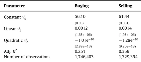
We take the estimates for these parameters fromBonaparte and Cooper (2010)who use monthly household account data to estimate these transactions costs for the buying and selling of common stocks. Their estimates are summarized in Table 1. As noted byBonaparte and Cooper (2010), only the fixed costs of trade are economically significant. Moreover, as these costs were estimated from the 1991–1996 time period which preceded the PSID data, the actual fixed costs of traders may be less than those estimated here.
3.2. Estimation
The preference parameters,ð
g
,bÞ, along with the opportunity cost of stock adjustment,c, are estimated using simulated method of moments. The estimates of trading costs fromTable 1as well as the stochastic processes for income and returns are inputs into this estimation. Finally, we discuss the procedure used to determine the borrowing limit,Ab.3.2.1. Moments
The estimation procedures seeks to match four moments. The data appendix provides detailed information about the sources and calculation of these moments. These moments are for stockholders only which is consistent with our model.
Table 1
Estimated trading costs.
Parameter Buying Selling
Constantni
0 56.10 61.44
ð0:05Þ ð0:061Þ
Linearni
1 0.0012 0.0014
ð1:63e06Þ ð1:93e06Þ
Quadraticni
2 1:01e10 1:28e10
ð2:88e13Þ ð9:26e13Þ
Adj.R2 0.251 0.359
Number of observations 1,746,403 1,329,394
The table reports estimates of the trading costs for buying and selling stocks. In parenthesis are the standard errors.
The first moment is the adjustment rate for shareholders of 46.7% biannually. This moment is particularly informative about the cost of stock trading, one of the key elements in our model. We calculate it from five waves of the PSID survey in the period of 1999–2007. The survey asked stockholders whether they bought or sold any non-IRA stocks since the previous interview. Within our sample, the percentage of stockholders that had positive answers ranged between 53% and 68% over the waves. This represents the gross adjustment rate. For these gross-adjustors, PSID further asked whether they put money into stocks, or took money out of them, or put about as much in as they took out. About 16.2% of the gross-adjustors reportedly put about as much in as they took out. On net, 46.7% of the stockholders either increased or decreased stock holdings, biannually from 1999 to 2007.7This net adjustment is consistent with the definition of stock adjustment in
our model. In contrast, the gross adjustment includes rebalance between different stocks which is not considered in our model.8
It should be noted that the 46.7% biannual adjustment rate is not convertible into a 23.5% annual adjustment rate, unless totally different households undertake stock adjustment in the two years. It might be, for example, that the same set of households adjust in both years, implying that the annual adjustment rate from PSID should also be 46.7%. We take this time aggregation into account in our estimation.
Bonaparte and Cooper (2010) calculate an adjustment rate of 71% from the Survey of Consumer Finance (SCF). The survey asks stockholders who own brokerage accounts how many times they bought or sold stock over the past year. InBonaparte and Cooper (2010), a stockholder is said to make stock adjustment if she bought/sold stocks at least once. The 71% annual gross adjustment rate is significantly higher than the 46.7% biannual gross adjustment rate in PSID. Notice that the SCF adjustment rate is for stockholders that own brokerage accounts, while the PSID adjustment is for all non-IRA stock holders. A higher adjustment rate in the SCF implies that stock holders that own brokerage accounts are more active traders.
The second moment is the portfolio composition of stockholders. We interpret bonds as the sum of deposits in transaction account and CDs, directly held bonds and saving bonds in the SCF. The data counterpart of stocks in the model is the amount invested in stocks (directly and indirectly) reported by SCF stock holders. Our measurement of stock share is ratio of mean stock holdings to mean financial wealth (stockþbond). The time series average of stock shares is 0.684. This moment is informative about the households’ degree of risk aversionð
g
Þand the opportunity cost of stock tradingðcÞ.The existing literature has found that a large coefficient of relative risk aversion is required in order to induce households to hold bonds due to the equity premium. We show that a smaller
g
coupled with a modest portfolio adjustment cost,c near unity and CðÞ small, induces sizable bond holdings, bringing the portfolio composition in the model close to the data.For the third moment, we follow the literature on intertemporal consumption and study the response of consumption growth to stock return movements. This moment, termed the ‘‘EIS’’, is computed from the consumption of shareholders, as inVissing-Jorgensen (2002a), with a point estimate of 0.298.
The fourth moment is the mean financial wealth–income ratio and is 2.43 in the data. This moment is important for estimating the discount factorband relative risk aversion
g.
9Intuitively a highbis associated with a high wealth–incomeratio because households value future consumption. Similarly a high
g
leads to high buffer-stock saving, hence a high wealth–income ratio.To estimate the parameters, we solve
G¼min ðg,b,cÞ
ðMsMdÞ0WðMsMdÞ: ð9Þ
HereMdare the moments from the data andMsare the simulated values of those moments for a given set of parameters,
ð
g
,b,cÞ.Wis the weighting matrix. Ideally, the weighting matrix should be the inverse of the variance–covariance matrix of moments from the data. But we are unable to calculate this weighting matrix because our moments come from different data sources. We use an identity matrix in the baseline estimation. In a robustness check, we use the inverse of the diagonal matrix whose entries are the variances of data moments. We demonstrate inSection 4.2that the estimates are robust to this alternative weighting matrix.The simulated moments are obtained by solving the household’s dynamic optimization problem through value function iteration. The solution method is described in the Appendix. Through simulation, a panel with 500 households and 800 time periods is created.10The simulated moments are calculated from this panel in exactly the same manner as they are calculated in the actual data. In particular, the adjustment rate is calculated bi-annually in the simulated data as it is in the PSID.
Throughout this analysis, we focus on financial wealth, ignoring housing and other durables. Further, the portfolio share relates to financial assets alone. The consumption measure includes the service flow from housing. This is consistent with a
7Bilias et al. (2010)also look at inaction in the PSID in an earlier sample but do not estimate adjustment costs. They look at the trading frequency of all respondents in the sample, including non-stockholders. As a results, they document much less frequent trading.
8Stock holdings in our model should be interpreted as the composite of individual stocks, such as the S&P 500. 9This is confirmed by the elasticity of moments with respect to parameters reported inTable 3.
model in which housing is rented by households who hold a portfolio of financial assets. This is also the outcome of a model in which the housing stock is held by households and is costlessly adjusted.
3.2.2. Results
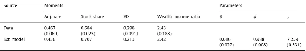
The results are presented inTable 2. The standard errors for the baseline estimates are computed from the matrix of numerical derivatives of the moments with respect to the parameters combined with the inverse of the variance matrix of the data moments, followingAdda and Cooper (2003). Moments from simulated data are indicated by the ‘‘Est. Model’’ row. These results are for the case of Ab¼0 so that households are unable to borrow on their bond accounts. The restriction ofAb¼0 comes from estimating this lower bound along with the other parameters of the model.11In the end, the best fit was with the tightest borrowing constraint ofAb¼0.
The simulated moments are all reasonably close to the actual data moments. The wealth–income ratio is met almost exactly. In contrast toHeaton and Lucas (1997), our model generates positive demand for low return riskless bonds. The share of bonds in total financial wealth is about 29%. The major reason for the increased demand for bonds is the costs of stock trading.
The estimation indicates that a discount factor of near 0.7 is necessary to match these moments. Traditional buffer-stock saving models, as inDeaton (1991)andCarroll (1992), typically use low discount factor. With a low discount factor, neither stocks nor bonds would be demanded in the absence of uninsurable income risks, thus the role of stochastic labor income is important here.Cagetti (2003)also estimatesbby matching wealth accumulation in the data and model, and reportsbvalues around 0.85.12Our estimate is lower for a number of reasons. First, wealth definition is narrower in our paper and income definition is broader, thus wealth–income ratio is lower.13Second, we include high return stocks in the model in addition to low return bonds, while in traditional buffer stock saving models as well asCagetti (2003), only low return bonds are available.
The estimate of
g
indicates a curvature of about 7.2, which is not the same as the inverse of the estimated EIS from the data. In the model with adjustment costs, there is no direct link between the inverse of the EIS and preference parameters. As we discuss below, the response of aggregate consumption growth to variations in the return depends on both the extensive (the choice of adjusting or not) and the intensive margins.The point estimate of the adjustment costs is 1c¼0:012. With average income of about $72,000 in the data used to estimate the trading costs reported in Table 1, this part of the adjustment costs is about $864. Combined with the estimated fixed cost of financial trades, the total fixed cost is around $920.
Table 3reports the elasticities of the moments with respect to the parameters. The table shows that wealth–income ratio is extremely sensitive tob. A 1% increase inbleads to almost 4% increase in wealth–income ratio. The adjustment
Table 2
Baseline estimation results.
Source Moments Parameters
Adj. rate Stock share EIS Wealth–income ratio b c g
Data 0.467 0.684 0.298 2.43
(0.069) (0.023) (0.091) (0.188)
Est. model 0.436 0.707 0.213 2.42 0.686 0.988 7.239
(0.027) (0.008) (0.531)
The table reports baseline estimation results. Stock share is the ratio of total stock over total financial wealth. EIS is the response of aggregate consumption growth to stock return from linear regression. Wealth–income ratio is the ratio of total financial wealth to total income. An identity matrix is used for estimation. In parenthesis are standard errors of moments and parameters, using the inverse of moment variances as a weighting matrix.
Table 3
Elasticities of moments to parameters.
Parameter Adjustment rate Stock share EIS Wealth–income ratio
b 0.803 0.033 1.079 3.875
c 24.35 4.625 5.242 0.797
g 0.226 0.833 0.316 1.731
The table reports the elasticities of moments to parameter values, defined as the percentage change of moments in response to a 1% change in parameter values.
11This was accomplished by re-estimating the model at different values ofAb 40.
12Alan (2006)also estimates the discount factor from a simulated method of moments approach. That analysis uses age dependent stock market participation rather than the financial wealth–income ratio.
rate is most responsive toc. Recall that ascincreases, the adjustment cost decreases. A 1% increase incleads to a 24.4% increase in adjustment rate, a 4.6% increase in stock share, and a 5.2% increase in EIS. These again highlight the importance of adjustment cost in our model. Although we emphasize that the inverse of
g
does not equal the inter-temporal elasticity of substitution, a higherg
is associated with less inter-temporal substitution. This is shown in the last row of the table—a higherg
leads to lower EIS and stock adjustment rate. The lower adjustment rate implies less consumption smoothing because a large part of stock adjustment is for the purpose of consumption smoothing, a point that will be further discussed inSection 5. Finally, a higherg
leads to a lower stock share and higher wealth–income ratio due to risk aversion.4. Robustness
This section examines the robustness of our findings. It includes estimation of alternative models of adjustment costs and the use of alternative moments due to measurement issues. Some additional simulations with different parameter-izations are also reported.
4.1. Alternative models of adjustment costs
The model assumes an adjustment cost that is proportional to income, reflecting the time cost of adjustment. Yet for some investors, the costs of adjustment may be better modeled as the payment of a fee to a broker who in turns makes the trades on behalf of the investor.14Or, as inBonaparte and Fabozzi (2011), investors may choose between two forms of adjustment: either a time cost or a fixed cost.
To study these alternatives, we revise the value of adjustment to be
vaðy,A
1R1Þ ¼ max AbZAb,AsZ0,n2f0,1g
uðcÞ þbER,y09R1,yvðy
0,A,RÞ, ð10Þ
with
c¼ X
i¼b,s
Ri1Ai1þy
n
ð1cÞyð1n
ÞFXi¼b,s
AiCðs1,sÞ: ð11Þ
From(11), if
n
¼1, we are back in the baseline formulation with the cost of adjustment being proportional to income. We call this the ‘‘Proportional AC’’ model in the discussion that follows. If, however,n
¼0, the adjustment costs is fixed atFunits of the consumption good. We term this the ‘‘Fixed AC’’ model. Finally, if we allow
n
2 f0,1gas a control, as in(10), then households have an additional control—the choice of the form of adjustment. In general, lower income households will choose the proportional cost while higher income households will choose the fixed adjustment cost technology. This is termed the ‘‘Mixed AC’’ case.There are two interesting dimensions to these alternative models of adjustment costs. The first has to do with the estimation of the parameters and the moment implications. We discuss that now. The second has to do with how the household responds to income shocks, a point we return to inSection 5.3.
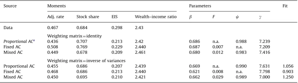
From the top section of Table 4, in the ‘‘Fixed AC’’ model, the estimates of bothb and
g
are close to the baseline estimates.15Since income has a mean of 1, the fixed cost estimateFis the fraction of average income lost in trading. It is about 0.7%. In the baseline model, the estimate of c¼0:988 implies that the income lost due to adjustment was 1.2%, higher than the fixed cost estimate.16The ‘‘Mixed AC’’ allows the household to choose between the forms of adjustment. The parameter estimates are not very different from the baseline either since the fixed cost of 0.012 is close to the estimated fraction of average income paid.
4.2. Alternative weighting matrix
Since we obtain data moments from different sources, it is impossible to calculate the inverse of the variance– covariance matrix of the moments which is often used as the optimal weighting matrix. Nevertheless, we can calculate the variances of data moments, and use the diagonal matrix whose entries are the inverse of these variances. The variances are 0.0048, 0.0005, 0.0082 and 0.0352 for adjustment rate, stock share, EIS and wealth–income ratio respectively. These are the squares of the standard errors of the data moments inTable 2. Using their inverses as weights, we put much more weight on stock share, and less weight on the wealth–income ratio compared to the identify matrix. Results are reported in the bottom section ofTable 4.
The results from re-estimating the baseline model are reported in the row labeled ‘‘Proportional AC’’ in the bottom section ofTable 6. Compared with results in the top section, neither the model moments nor parameter values exhibit
14We are grateful to the referee for suggestions which led to the development of this section.
15The top section ofTable 4reports results from using the identity matrix while the bottom section, discussed below, reports estimates using a weighting matrix.
large changes. The estimated value ofbis a bit lower and the curvature of the utility function a bit larger. The adjustment rate and stock share are slightly better matched, because they are given more weight. The fit (distance from model and data moments) of the model is 1.056. If the diagonal weighting matrix is the optimal one, with one degree of freedom, the
p-value is 0.3042 and the model is statistically rejected.17
The remainder ofTable 4continues with the alternative models of adjustment costs, now estimated with a weighting matrix. As with the baseline specification, the weighting matrix leads to modest changes in the estimates, notably a reduction inb. The ‘‘Fixed AC’’ model actually fits the moments a bit better while the ‘‘Mixed AC’’ case fits the moments worse relative to the baseline.
4.3. Measurement
As discussed at some length in Appendix, our moments come from different sources and thus there is no consistent sampling frame.18In particular, the SCF, which is the source for our stock share and wealth–income ratio moments, is
known for oversampling of rich households. The SCF provides weights to all the respondents, with the rich ones receiving smaller weights so that the weighted sample is nationally representative. As discussed inKennickell (2008), the wealthy are oversampled in the SCF in part to offset the low response rate from the rich respondents, and to obtain more precise information about the wealthy. But, the adjustment rate moment comes from the PSID where oversampling of the wealthy is not an issue.
In general, as long as the choice of weights is consistent between the calculation of moments from the real data and the simulated data, the choice between weighted and unweighted sampleper seis not problematic for a simulated method of moments approach. However, for our exercise, as the data come from different sources, differences in these data sets and thus in the sampling frame that underlies the moments calculated from them could be problematic.
We are less concerned here for a few reasons. First, there is no response problem in simulated data. Thus if the oversampling in the SCF is partly to compensate for low response rates, then the unweighted moments from SCF is actually more consistent with the adjustment rate from PSID and simulated moments in the sampling frame. Second, as we will demonstrate, the parameter estimates are largely robust to changes in the ways the moments are measured. The one exception is that our estimate ofbis, not surprisingly, sensitive to the measured wealth–income ratio.
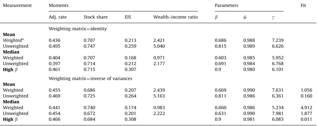
As noted earlier, the baseline model matched the means of stock share and wealth–income ratio from a weighted SCF sample. Alternative moments for the SCF, with and without weighting and matching medians rather than means, are presented in Table 5. Since the weighting is an attempt to offset oversampling of wealthy households, the weighted wealth–income ratios are lower for both means and medians compared to the unweighted. The median shares are lower than the average shares, indicating some skewness in the distribution. The big difference in these moments comes from the wealth–income ratio, not from the shares.
Table 6presents the estimation results from these alternative SCF moments. The simulated moments for the various SCF measures should be compared with the actual moments reported inTable 5. The top section of the table is for the identity weighting matrix and the bottom section uses the inverse of the variances as weights.
Table 4
Robustness of estimation—alternative adjustment cost.
Source Moments Parameters Fit
Adj. rate Stock share EIS Wealth–income ratio b F c g
Data 0.467 0.684 0.298 2.43
Weighting matrix¼identity
Proportional ACa 0.436 0.707 0.213 2.42 0.686 n.a. 0.988 7.239
Fixed AC 0.508 0.769 0.229 2.440 0.687 0.007 n.a. 7.209
Mixed AC 0.449 0.678 0.209 2.461 0.680 0.012 0.983 7.416
Weighting matrix¼inverse of variances
Proportional AC 0.455 0.686 0.207 2.439 0.669 n.a. 0.990 7.631 1.056
Fixed AC 0.468 0.686 0.213 2.440 0.621 0.008 n.a. 7.798 0.903
Mixed AC 0.450 0.695 0.210 2.421 0.662 0.029 0.989 7.000 1.250
The ‘‘Proportional AC’’ case includes only proportional adjustment costs. This is the same as the baseline when the identify matrix is used. The ‘‘Fixed AC’’ rows report results from estimatingðb,F,gÞ. The ‘‘Mixed AC’’ rows report results from a model in which households can choose between fixed adjustment cost (F) and proportional adjustment costc. The last column labeled ‘‘Fit’’ reports the distance between model and data moments, weighted by the inverse of variance of the data moments.
aThis is the baseline case.
Except forb, the parameter estimates are fairly robust across these competing ways of calculating the SCF moments. As the median weighted wealth–income ratio is low relative to the other cases, the estimate of b is much lower. The opposite is true for the mean unweighted case where the high financial wealth–income ratio translates into a higher estimate ofb.
To further gauge the importance of the measurement of the wealth–income ratio, we drop this moment and re-estimate the model to see how the results change. Since that moment pinned downb, we setb¼0:90 and estimated
ðc,
g
Þfrom the remaining three moments.The results, reported in the row labeled ‘‘Highb’’, indicate a value ofc a bit below the baseline estimate and less curvature than the baseline. Model moments change slightly towards a better fit.
The bottom section ofTable 6reports this estimation exercise using the alternative weighting matrix. Again, compared with the results using identity matrix, no significant difference is found. For the ‘‘Highb’’ case, the fit is 0.0011 and thep
value is 0.92. Had the diagonal matrix been optimal, we could not reject the model at 10% level.
4.4. Alternative parameterizations
In the following experiments, we explore how the simulated moments change as we vary the exogenous processes, including mean income level, stochastic process of income shocks and bond return. The results are reported inTable 7.
Table 5
Alternative SCF moments.
Measurement Stock share Wealth–income ratio
Mean
Weighted 0.684 2.430
Unweighted 0.7215 5.028
Median
Weighted 0.572 0.973
Unweighted 0.566 2.195
The ‘‘Stock Share’’ and ‘‘Wealth–Income Ratio’’ moments from the SCF are computed in two ways. Either by taking both time series and cross-sectional means or by taking the means over time of the cross-sectional median. In the table, the first method is labeled ‘‘Mean’’ and the second is labeled ‘‘Median’’. The moments are calculated with and without sample weights. For the medians, SCF weights are added up, and the median household is the household that corresponds to the half of the sum of weights.
Table 6
Robustness of estimation—different SCF moments.
Measurement Moments Parameters Fit
Adj. rate Stock share EIS Wealth–income ratio b c g
Weighting matrix¼identity Mean
Weighteda 0.436 0.707 0.213 2.421 0.686 0.988 7.239
Unweighted 0.495 0.747 0.259 5.040 0.815 0.989 6.626
Median
Weighted 0.404 0.707 0.168 0.971 0.603 0.985 5.952
Unweighted 0.397 0.714 0.212 2.177 0.691 0.984 6.768
Highb 0.461 0.715 0.307 0.9 0.980 6.101
Weighting matrix¼inverse of variances Mean
Weighted 0.455 0.686 0.207 2.439 0.669 0.990 7.631 1.056
Unweighted 0.469 0.725 0.264 5.163 0.811 0.986 6.361 0.160
Median
Weighted 0.441 0.740 0.174 0.983 0.660 0.986 5.234 4.912
Unweighted 0.454 0.672 0.201 2.222 0.631 0.990 7.981 1.877
Highb 0.466 0.684 0.308 0.9 0.981 6.083 0.011
The different experiments labeled as rows correspond to the four different measures of the SCF moments reported inTable 5. The other moments used are the same as inTable 2. The row labeled ‘‘Highb’’ drops the wealth–income ratio moment and setsb¼0:9. In this experiment the parametersðc,gÞare estimated from three moments, excluding the wealth–income ratio and using the weighted mean for the share. The last column labeled ‘‘Fit’’ reports the distance between model and data moments, weighted by the inverse of variance of the data moments.
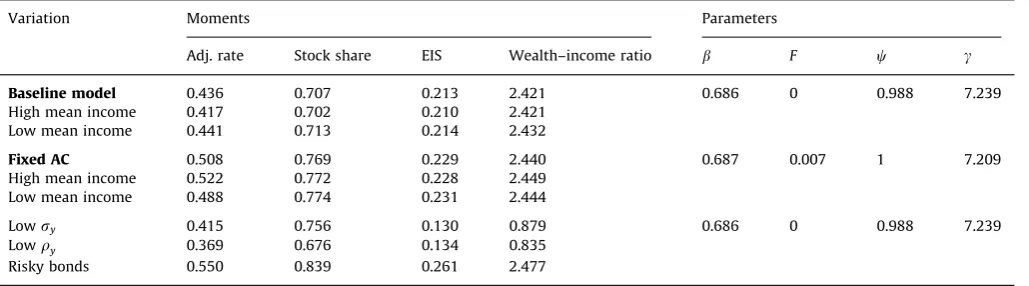
The first two blocks of the table show how the moments respond to changes in mean income level, using the baseline estimates and the ‘‘Fixed AC’’ cases.19The ‘‘High Mean Income’’ treatment increases average income by 20% and the ‘‘Low Mean Income’’ treatment reduces it by 20%. Else, the same stochastic progress for income, explained in Appendix, is used. Given that the adjustment cost is proportional to income, adjustment is more costly for the high income group than for the low income group. But, the gains to adjustment will also depend on mean income through the size of the portfolio. As seen in the top block ofTable 7, the first effect dominates—the adjustment rate is a bit lower for the high mean income treatment and a bit higher for the low mean income treatment relative to the baseline. There is some response in other moments as well. None of these effects is large.
But in the fixed adjustment cost model, the pattern reverses. Given that the cost of adjustment is independent of income, the high mean income households adjustment more frequently while the low income households adjust less frequently. These responses to income differentials are slightly larger than they were (and in the opposite direction) in the baseline case.
The procedure used to generate our approximation of the household income process is outlined in Appendix. The process we use is more persistent and more volatile than in some other studies. For example,Heaton and Lucas (1997) assume a serial correlation of 0.53 and standard deviation of income innovations equal to 0.24. We study how the simulated moments change with alternative income processes. The ‘‘Low
s
y’’ case replaces the income process estimatedin the PSID with one in which the innovation to the income process is 0.20 rather than 0.29 in the baseline. The portfolio choice literature has both empirical evidence and theoretical argument that less risky labor income should be associated with less saving and more investment in risky assets. This is also found in our model—from the baseline case, the financial wealth–income ratio decreases from 2.421 to 0.879, and the stock share rises from 0.707 to 0.756 in the ‘‘Low
s
y’’. So whilewe can still generate bond holdings, it is clear that this share is sensitive to the volatility of the income process due to the presence of portfolio adjustment costs.
The ‘‘Low
r
y’’ case replaces the persistence parameter of income shocks of 0.842 with 0.60. This has very similar effects as the experiment with less volatile income innovations. This is partly by construction since the reduction in the serial correlation generates less volatile income, given the same standard deviation of the income innovations. Still, in this case the stock share remains close to that in the estimated model as does the adjustment rate. But the wealth–income ratio is much lower.The last row ofTable 7, labeled ‘‘Risky Bonds’’, reports moments when the return on bonds is stochastic. The bond process is estimated from Shiller data for the sample period of 1947–2007. The mean return is 2%, the standard deviation of the innovation is 0.0266 and the serial correlation is 0.57. This contrasts with the zero serial correlation of stock returns. The moments change from the addition of these shocks to the model.20Not surprisingly, the stock share rises since bonds are no
longer safe and the adjustment rate increases as well due to the additional uncertainty. But the financial wealth–income ratio changes only slightly, indicating that risks of bonds return change the portfolio composition, but not total savings.
5. Responses to shocks
Given these estimates: how do households respond to income and return shocks? This is a traditional question of the consumption and portfolio choice literature and is a main question of this study. Our answer differs because of the presence of portfolio adjustment costs.
Table 7
Robustness of moments.
Variation Moments Parameters
Adj. rate Stock share EIS Wealth–income ratio b F c g
Baseline model 0.436 0.707 0.213 2.421 0.686 0 0.988 7.239
High mean income 0.417 0.702 0.210 2.421
Low mean income 0.441 0.713 0.214 2.432
Fixed AC 0.508 0.769 0.229 2.440 0.687 0.007 1 7.209
High mean income 0.522 0.772 0.228 2.449
Low mean income 0.488 0.774 0.231 2.444
Lowsy 0.415 0.756 0.130 0.879 0.686 0 0.988 7.239
Lowry 0.369 0.676 0.134 0.835
Risky bonds 0.550 0.839 0.261 2.477
‘‘Fixed Cost’’ denotes model of fixed adjustment cost. ‘‘High Mean Income’’ is the same as the baseline income process with a 20% higher mean. ‘‘Low Mean Income’’ is the same as the baseline income process with a 20% lower mean. The ‘‘Lowsy’’ case reduces the standard deviation of the income innovation to 0.20 from the baseline of 0.29. The ‘‘Lowry’’ case reduces the serial correlation of the income process to 0.60 from the baseline of 0.842. The ‘‘Risky Bonds’’ case introduces a stochastic process for bonds with a mean of 2%, a standard deviation of the innovation of 0.0266 and a serial correlation of 0.57.
19As suggested by the referee, these differences may reflect income differentials across households of different education levels.
We first present and discuss the policy functions of our estimated model. We then turn to simulation results to display the properties of these policy functions.
5.1. Policy functions
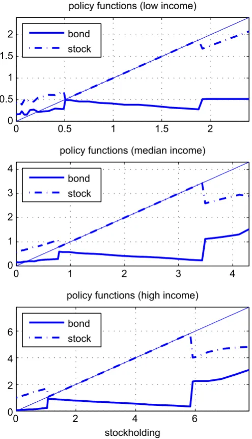
Fig. 1shows the decision rules (policy functions) for future stock and bond holdings as a function of current stock holdings. Here, the measure of current stock holdings includes the realized return on stocks: in the notation of the model this isAs1Rs
1. The decision rules are shown for three different realizations of income. Current period’s bond holdings are
fixed at the average of the simulated panel and the return state is at its mean of 6.33%.
The decision rules are plotted together with the 451line. Given the inaction in stock adjustment created by the non-convex adjustment costs, future stock holdings can be the same as current stock holdings, indicated by decision rules which coincide with the 451line.21
The upper panel is for a household whose income realization is at the low level, one standard deviation below the mean. The middle panel is for a household whose income realization is at the mean. The lower panel is for a household whose realized income is one standard deviation above the mean.
As indicated in these policy functions, there is a sizable inaction region for stock adjustment for all three income states. It is only in the tails of the current stock holdings that adjustment in this margin occurs. Over these regions of inaction, in
0 0.5 1 1.5 2
0 0.5 1 1.5 2
policy functions (low income)
bond stock
0 1 2 3 4
0 1 2 3 4
policy functions (median income)
bond stock
0 2 4 6
0 2 4 6
policy functions (high income)
stockholding bond
stock
Fig. 1. Policy functions. This figure shows the policy functions for three different income states. Current stock holdings (including current returns)
are shown along the horizontal axis. Future stock and bond holdings are indicated along the vertical axis.
which the stock return is re-invested automatically, bond holdings are decreasing functions of the stock holdings. As the value of the stock account increases, households will consume at a higher level. This is financed through reducing bond holdings.Thus bond holdings are valuable even though the bond return is much lower than the stock return.
The size of the inaction region also depends on the income shock. In the high income state, the critical values of current stock holdings defining the inaction region are higher, and the inaction range is broader. In the regression of simulated data below, adjustment probability decreases with income, which is consistent with the policy rules here. It is optimal to increase stock holdings when income is in the high state, which is partly done by the ‘‘inaction’—the automatic reinvestment of stock return. By contract, when low income states necessitate running-down of stock holdings, it needs to be done through adjustment.
When adjustment of the stock account does occur, the bond holdings move in the opposite direction. For example, when households in high income state find it optimal to reduce their stock accounts for higher consumption.They also increase bond holdings so that consumption can be smoothed out of bonds in the future inaction periods.
As indicated inFig. 1, the bond policy function is very non-linear even though the adjustment costs only apply to stocks. Of course, once the adjustment cost is paid for stocks, then the choice of bond holdings is quite different from the states of no adjustment in stocks.22
5.2. Simulation results
To illustrate the choice problem of households, we study some simulation results. This enables us to see the response to households to income and return shocks. These responses indicate how households use their portfolios to smooth consumption and rebalance their portfolio in response to income and return variations.
The figures, which summarize the simulations, show stock holdings, bond holdings and consumption as control variables over time. Further, the stock holdings series are marked by diamonds in periods of inaction.
5.2.1. Response to income shocks
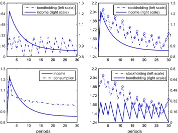
Given the presence of adjustment costs, the response to income shocks is nonlinear. Accordingly we distinguish the response of the household to a relatively small income shock as shown inFig. 2, from the response to a large income shock, as shown in Fig. 3. A small income shock is a realization that is one-third of standard deviation away from the mean income, while a large income shock is one standard deviation away. For either exercise, we set the initial stock holdings and bond holdings to the mean levels in the simulated data.
bondholding (left scale) stockholding (left scale)
stockholding (left scale)
5 10 15 20 25 30
0 0.16 0.32 0.48 0.64 0.8
5 10 15 20 25 300.8
0.9 1 1.1 1.2 1.3
income (right scale)
5 10 15 20 25 30
1.24 1.4 1.56 1.72 1.88 2.04 2.2
5 10 15 20 25 300.8
0.9 1
1.1 1.2 1.3
income (right scale)
5 10 15 20 25 30
0.8 0.9 1.1 1.2 1.3
periods
income consumption
5 10 15 20 25 30
1.24 1.56 1.72 1.88 2.04 2.2
periods
5 10 15 20 25 300
0.16 0.32 0.48 0.64 0.8
bondholding (right scale)
1
1.4
Fig. 2.Small income shock. The figure plots the dynamics of stock holdings, bond holdings and consumption in response to a small income shock.
The stock return is fixed at the average level (6.33% per year). Diamonds mark inaction of stock account adjustment.
As indicated in the top left panel ofFig. 2, a household’s bond holdings increase with an small income shock. From the bottom left panel, there is also an increase in consumption at the time of the shock. Since the income shock is relatively small, stock holdings do not instantly change, as indicated by the top right panel. Instead, stock holdings build through the reinvestment of dividends without any adjustment (as indicated by the diamonds). In the subsequent periods, bond holdings are decreased to fund consumption. After a few periods, the stock account has grown enough to warrant an adjustment. At the time of adjustment (periods 5, 10, etc.), the stock account falls and the bond account increases, as shown in the bottom right panel. This interaction between the bond and stock accounts is reminiscent of the standard Baumol–Tobin model of money demand.
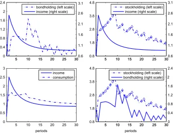
The response to a large income shock is somewhat different. Looking at the top right panel ofFig. 3, the large income shock induces an immediate stock adjustment. The increase in the stock account is accompanied by a decrease in the bond account, shown in the top left panel. From period 2 until period 9, the stock account is not adjusted. Bond holdings are increased in period 2 through 5 as income realizations are still high, then it is reduced, again to finance additional consumption from gains in the stock market. Since then the usual dynamic of portfolio rebalancing occurs again, as shown in the bottom right panel. Responses of consumption to large and small income shocks are very similar.
Thus these figures combine two effects. The first is the response of consumption and asset holdings to the income shocks. The second is the ongoing interaction between the stock and bond accounts. Due to the adjustment costs, there is a natural dynamic of infrequent adjustment between the stock account and the bond account (portfolio rebalancing) along with the financing of consumption from the bond account (consumption smoothing). It is particularly interesting to note how the changes in bond holdings complement stock holdings, which leads to a negative comovement between the two assets in general. In the presence of two assets, consumption is very effectively smoothed, although it has a slightly larger variation in response to a larger income shock.
5.2.2. Response to return shocks
We now study the response of households to return shocks. This is illustrated inFig. 4. For this simulation, income is held at its mean and initial stock holdings and bond holdings are both the averages of the simulated panel.
Households generally increase (decrease) their stock holdings, bond holdings and consumption in response to a positive (negative) shock to stock return. Nevertheless, the adjustment in asset holdings is large relative to consumption. This response shows both consumption smoothing and portfolio rebalancing at work. The positive comovement of consump-tion with stock return is echoed by the positive coefficient from regressing consumpconsump-tion growth rate on stock return.
However, the comovement of return with either stock or bond holdings is complex. The upper-right panel shows that stock adjustment is very infrequent. During the inaction, the bond account is adjusted, either in the same direction as the return or the opposite. The correlation coefficient between bond holdings and stock holdings is 0.2666, indicating that the negative comovement dominates, which is clear in the lower-right panel. For example, suppose stock holdings are high
5 10 15 20 25 30
0 0.4 0.8 1.2 1.6 2 2.4
5 10 15 20 25 300.6
1.1 1.6 2.1 2.6 3.1 bondholding (left scale) income (right scale)
5 10 15 20 25 30
0.8 1.8 2.8 3.8 4.8
5 10 15 20 25 300.6
1.1 1.6 2.1 2.6 3.1 stockholding (left scale) income (right scale)
5 10 15 20 25 30
0 0.5 1 1.5 2 2.5 3 periods income consumption
5 10 15 20 25 30
0.8 1.8 2.8 3.8 4.8 periods
5 10 15 20 25 300
0.4 0.8 1.2 1.6 2 2.4 stockholding (left scale) bondholding (right scale)
Fig. 3. Large income shock. The figure plots the dynamics of stock holdings, bond holdings and consumption in response to a large income shock.
and there is a high stock return. If a household decides not to adjust its stock account, it is always optimal for the household to reduce bond holdings to finance consumption.
Fig. 5shows the aggregate implications of this experiment. The aggregate level response of control variables to return shocks is quite different. The difference in correlations are shown inTable 8.
There are two points to note. First, at the aggregate level, both stock and bond holdings are more correlated with the return, but consumption is less correlated with the return. This shows that aggregate consumption is smoother as it is less responsive to the stock return, which in turn is made possible by the higher responsiveness of asset holdings to stock return.
bondholding (left scale) stockholding (left scale)
stockholding (left scale)
10 20 30 40
−0.1 0.1 0.3 0.5 0.7 0.9 1.1 1.3
10 20 30 400.9
1.1 1.3 1.5
stock return (right scale)
10 20 30 40
0.75 1.25 1.75 2.25 2.75
10 20 30 400.9
1.1 1.3 1.5
stock return (right scale)
10 20 30 40
0.8 0.9 1 1.1 1.2 1.3 1.4 1.5 periods stock return consumption
10 20 30 40
0.75 1.25 1.75 2.25 2.75 periods
10 20 30 40−0.1
0.1 0.3 0.5 0.7 0.9 1.1 1.3
bondholding (right scale)
Fig. 4.Return shocks and individual decisions. The figure plots the dynamics of individual stock holdings, bond holdings and consumption in response
to shocks to stock return. Income is fixed at its mean level.
bondholding (left scale)
10 20 30 40 1.3 1.8 2.3 2.8 3.3 3.8
10 20 30 400.9 1.1 1.3 1.5 stockholding (left scale)
consumption (left scale) stockholding (left scale) 10 20 30 40
0.5 0.7 0.9 1.1 1.3 1.5 1.7
10 20 30 400.9 1.1 1.3 1.5
stock return (right scale) stock return (right scale)
10 20 30 40 1 1.2 1.4 1.6 1.8 periods
10 20 30 400.9 1.1 1.3 1.5
stock return (right scale)
10 20 30 40 1.3 1.8 2.3 2.8 3.3 3.8 periods
10 20 30 400.5 0.7 0.9 1.1 1.3 1.5 1.7
bondholding (right scale)
Fig. 5. Return shocks and aggregate decisions. The figure plots the dynamics of aggregate stock holdings, bond holdings and consumption in response
Second, at the aggregate level the correlation between stock and bond holdings is clearly positive. In fact, it equals 0.875 in contrast to the negative correlation found at the household level. The aggregate correlation has a different sign since the aggregation smooths over the lumpy portfolio adjustment at household level.23
At the aggregate level, we can calculate adjustment rate at any point of time. We find that the adjustment rate is positively correlated with return. This is due to economics of scale—high return increases portfolio size, which makes adjustment more worthwhile. Since a larger portfolio implies more consumption, the adjustment rate and consumption are also positively correlated. The comovement of consumption and stock returns, amplified by the adjustment decision, underlies the regression results used as a moment inTable 2.
5.3. Regression results
For further evidence on the structure of household decision rules, we study the state-dependence of bond holdings, stock holdings and consumption as well as the adjustment decision through a regression structure. Although the regressions are only coarse approximations, they are illustrative of the forces at work.
We characterize the decision rules for the baseline, the fixed adjustment cost and highbmodels introduced earlier. The comparison between the baseline and fixed cost models shows how the decisions depend on the structure of adjustment costs. The comparison between baseline and highbmodel mostly shows how the decisions are affected by wealth–income ratio. These regressions are run at the household level from the same simulated panel used to calculate our moments. Results are reported inTables 9 and 10. Since all the regression coefficients are highly significant, standard errors are not reported in the tables.
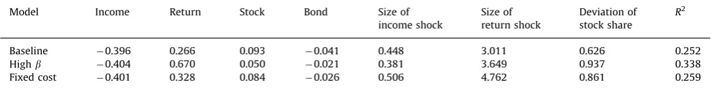
5.3.1. Extensive margin decisions
Table 9reports the extensive margin decision—whether to adjust stock account or not. The decision is regressed on four state variables (income, stock return, stock holdings and bond holdings) and three nonlinear transformation of state variables. ‘‘Size of income shock’’ is defined as the absolute distance of realized income from mean income:9yy9wherey is the mean income in the simulated data. ‘‘Size of return shock’’ is defined as the absolute distance of realized stock return from mean return, multiplied by the stock share:9Rs
Rs9As
=ðAsþAbÞ. ‘‘Deviation of stock share’’ is defined as the absolute distance of stock share from the average stock share in simulated data.24This regressor is included because we interpret
non-adjustment as being in the inaction region, and the average stock share is a proxy for the center of inaction region. For each of the three models, the coefficients have the same signs. Adjustment is less likely in high income states. When income is high, it is optimal to increase stock holdings, which is automatically done as the stock return is reinvested. The adjustment probability increases with stock holdings and stock return, because the benefit of adjustment increases
Table 8
Individual and aggregate correlations.
Data corrðRs,As
Þ corrðRs,Ab
Þ corrðRs,cÞ
corrðAs,AbÞ
Individual 0.455 0.149 0.534 0.267
Aggregate 0.567 0.216 0.430 0.875
This table shows the correlations at the individual and aggregate levels in response to stock return shocks. Income shock is shut down, with income level being fixed at the mean.
Table 9
Regression—adjustment decision.
Model Income Return Stock Bond Size of
income shock
Size of return shock
Deviation of stock share
R2
Baseline 0.396 0.266 0.093 0.041 0.448 3.011 0.626 0.252
Highb 0.404 0.670 0.050 0.021 0.381 3.649 0.937 0.338
Fixed cost 0.401 0.328 0.084 0.026 0.506 4.762 0.861 0.259
The table reports regression of adjustment decision on state variables: income, stock return, stock holdings and bond holdings. Three nonlinear transformation of state variables are also included in the regression. ‘‘Size of income shock’’ is defined as the absolute distance of realized income from mean income. ‘‘Size of return shock’’ is defined as the absolute distance of realized return from mean return, multiplied by stock share. ‘‘Deviation of stock share’’ is defined as the absolute distance of stock share from the average stock share in simulated data. All the regression coefficients are highly significant and standard errors are not reported. The ‘‘Baseline’’ model is presented inTable 2, the ‘Highb’’ model is presented inTable 6and the ‘‘Fixed Cost’’ model is presented inTable 4.
with stock holdings due to economies of scale. Bond holdings are a cushion against income and return shocks, so it decreases the likelihood of adjustment.
Both the size of income and return shocks have positive impacts on adjustment. These results are consistent with the patterns of consumption smoothing and portfolio rebalancing illustrated above. The adjustment probability increases with the deviation of stock share. When a household’s stock share is far from the mean, it is likely to be out of the inaction region, and adjustment becomes necessary.
Compared with the baseline model, the highbmodel has a much larger coefficient on the deviation of stock share. This is again because the benefit of adjustment increases with portfolio size, thus households in the highb model are less tolerant to deviation from the optimal share. Further, with a large portfolio, the income shock becomes less important, but the return shock becomes more important. This is also reflected in the regression coefficients.
In the fixed cost model, since the estimated adjustment cost is smaller than in the baseline, adjustment decision is more sensitive to income shocks, return shocks and deviation of the stock share.
5.3.2. Intensive margin decisions
Table 10 reports the regressions results on the intensive margin. The regressors are state variables plus a constant. We split households into adjustors and non-adjustors. This is consistent with the households optimization problem—after a household chooses to adjust or not, it makes decisions on the intensive margin as well. Each regression yields a very high R-squared, indicating highly linear decision rules.
Adjustors and non-adjustors have quite different decision rules. The most distinctive difference is with bond decisions. For adjustors, bond holdings are positively correlated with stock holdings and stock return, which is due to the usual portfolio rebalancing. But, for non-adjustors the correlation is negative, which echoes the mechanism illustrated in the policy functions (Fig. 1). Namely, during periods of inaction households run down bond holdings to finance consumption induced by stock returns.
For adjustors, bond holdings are much less responsive to income than for non-adjustors who rely on bonds to absorb income shocks. Consumption of adjustors is more responsive to income and stock return shocks. But the difference is small, reflecting consumption smoothing.
All the regression coefficients have the same signs across different models, except that bond holdings decrease with income in the fixed cost model. As noted inHeaton and Lucas (1997), labor income has a relative low risk and functions like bonds. When the adjustment cost is not proportional to income, income is a good substitute for bond holdings. In addition, the income shock is persistent. Thus in the fixed cost model, it is optimal to reduce bond holdings when income is high. A parallel effect is the much higher response of stock holdings to income shocks in the fixed cost model. Compared with the baseline, the highbmodel’s consumption is much less responsive to income, but more responsive to stock return. This is again due to the higher wealth–income ratio which dwarfs the importance of income relative to
Table 10
Regression—intensive margin decision.
Choice Income Return Stock Bond R2
Adjustor
Consum.
Baseline 0.389 0.265 0.139 0.114 0.984
Highb 0.246 0.620 0.065 0.047 0.990
Fixed cost 0.388 0.274 0.150 0.094 0.986
Bond
Baseline 0.094 0.852 0.348 0.593 0.857
Highb 0.007 4.530 0.255 0.700 0.975
Fixed cost 0.028 0.824 0.291 0.679 0.908
Stock
Baseline 0.562 0.786 0.607 0.348 0.908
Highb 0.210 0.441 0.069 0.042 0.982
Fixed cost 0.647 0.815 0.654 0.286 0.945
Non-adjustor
Consum.
Baseline 0.373 0.226 0.148 0.099 0.984
High beta 0.210 0.441 0.069 0.042 0.982
Fixed cost 0.358 0.259 0.159 0.084 0.985
Bond
Baseline 0.626 0.226 0.148 0.921 0.997
High beta 0.790 0.438 0.068 0.977 1.000
Fixed cost 0.642 0.258 0.159 0.937 0.996
asset return. Consumption response to stocks holdings appears to be smaller, but this is due to the large-scale stock holdings in the high b model. Measured by the regression coefficient multiplied by stock holdings, the response of consumption to stock holdings is much larger in the highbmodel.
These basic patterns hold when we use parameters from the alternative measure of SCF moments and alternative weighting matrix. In summary, we find the consumption smoothing and portfolio rebalancing mechanisms presented here are robust.
5.4. Substitution between stocks and bonds—data evidence
One of the most notable phenomena in the simulation results is the substitution between stock and bond holdings, which is a direct result of the infrequent adjustment of the stock account due to non-convex adjustment costs.
Specifically, when the stock account is not adjusted, bond holdings are adjusted for consumption smoothing purposes. This typically results in a negative correlation between changes in stock holdings and bond holdings, because the stock return is positive on average and non-adjustment means an increase in the stock account. The negative correlation also arises when stock holdings are too high and adjustment takes place. In this case stock holdings are reduced, while bond holdings are replenished.
We look at PSID data and find evidence supporting this negative correlation. Since 1999, the PSID provides wealth supplements bi-annually. Thus we employ the panel structure of data on stock holdings, bond holdings and income to study their correlations. Data description and sample selection criteria are given in Appendix.
We pool data from different years and regress income, bond holdings and stock holdings on age, age-squared, education dummies and sex-of-head dummy. The residuals, denotedyi,t,Bi,tandSi,trespectively, are income, bond holdings and stock
holdings with demographics controlled for, and thus are comparable with simulated data. DefineDBi,t¼Bi,tBi,t1, then
DBi,t is the change in bond holdings, which can be obtained from PSID data. We also obtainDyi,t andDSi,t from the data,
and calculate correlations betweenDyi,t,DBi,tandDSi,t. The same correlations are also calculated from the simulated data.
Notice thattrepresents two years because surveys take place every two years.
Table 11 reports the correlations both in the data and the model, together with bootstrapped standard errors. The correlation between changes in stock holdings and bond holdings is negative,0.338 in the data and0.534 in the model, both are statistically significant. The correlations betweenDyt andDSt are positive and statistically significant, both in the
data and model.
The correlation betweenDyt andDBt is slightly negatively in the data, not statistically significant at 5% level. In the
model it slightly positive. The explanation for the low correlation is offered inFigs. 2 and 3. Bond holdings increase with small income shocks, but decreases with large income shocks, so the net effect is small.
6. Conclusion
Portfolio adjustment costs influence a household’s responses to income and return shocks. The opportunity cost of stock trading, along with the discount factor and curvature in preferences, are estimated via simulated method of moments. The presence of adjustment costs is necessary to match both the portfolio share of stock in financial wealth and the low stock adjustment rate.
A household’s response to shocks comes in two forms: portfolio rebalancing and consumption smoothing. The response is highly nonlinear. The stock account is adjusted in response to large income shocks while the bond account buffers consumption from smaller shocks. Our simulation results reveal a strong negative correlation between stock and bond holdings at the household level. When households refrain from adjusting stock accounts to avoid costs, their stock account is increased due to the re-invested dividend, but the bond account is run down to finance consumption. On the other hand, when stock adjustment occurs, the bond account is replenished. Evidence in the PSID supports such substitution.
Shocks to stock returns lead to mild variations in consumption, but large-scale changes in both bond and stock holdings. Due to inaction in stock trading, household stock holdings and bond holdings exhibit slightly negative correlation
Table 11 Correlations.
Variable Data Model
Dyt DBt DSt Dyt DBt DSt
Dyt 1 1
DBt 0.062 1 0.090 1
(0.036) (0.003)
DSt 0.117 0.338 1 0.180 0.534 1
(0.015) (0.072) (0.003) (0.005)