Effect of NTL on Power System Losses at Industrial Load

(1)

Effect of NTL on Power System Losses at Industrial

Load

Deepak Madan

Deptt. of Electrical & Electronics Engg, DVIET, Karnal (Haryana),

India

Meenakshi Dhakla

Asstt. Prof., Deptt. of Electrical & Electronics Engg, DVIET, Karnal

(Haryana), India

Balvinder Dhull

Deptt.of Electrical Engg, AIET,

Faridkot (Punjab), India

Abstract–Merely generating more power is not enough to meet present day requirements. Power consumption and losses have to be closely monitored so that the generated power is utilized in an efficient manner. This illegal electricity usage may indirectly affect the economic status of a country. Also the planning of national energy may be difficult in case of occurrence of T& D Losses. The T&D Losses have been quite high in India. The reasons cited for such high losses are; lack of adequate T & D capacity, too many transformation stages, improper load distribution and extensive rural electrification etc. In addition defective metering, un-metered supply, and pilferage have resulted in high Non-Technical Losses (NTL). The purpose of this paper is to investigate NTL in power systems. These are losses in power systems that cannot be predicted or calculated ahead. Non-technical losses can also be viewed as undetected load of customers that the utilities don’t know. When an undetected load is attached to the system, the actual losses increase while the losses expected by the utilities will remain the same. In this paper, Residential & Industrial loads (operated at 11KV known as primary distribution system) are considered at node1 and node2 respectively in 3-bus system & NTL load is added to the industrial load and power system losses are measured.

Keywords–NTL, Power System Losses, Industrial Load.

I. I

NTRODUCTION

Economic Progress of any country depends on the fundamental amenities, skilled and available employees. Electricity is one of the basic infrastructures which accelerate the growth rate. This makes energy resources extremely significant for energy country in the world. In bringing energy needs and energy availability into balance, there are two main elements such as energy demand and energy supply. In this regard, every country should put efforts to attain such a balance and hence conduct research and development studies to develop its own energy conservation programs for the existing and new energy resources. India is immerging nation with respect to industrial and economic developments. In India, average T&D losses; have been officially indicated as 23 percent of the electricity generated. However, as per sample studies carried out by independent agencies including TERI, these losses have been estimated to be as high as 50 percent in some states. In a recent study carried out by SBI Capital Markets for Delhi Viduit Board DVB, the T&D losses have been estimated as 58%. This is contrary to claims by DVB that their transmission and distribution losses are between 40 and 50 percent. The T&D losses in the advanced Countries of the world ranging from 4-12%. However, the T&D losses in India are not comparable with advanced countries as the system

operating conditions are different in different countries [1]. With the setting up of State Regulatory Commissions in the country, accurate estimation of T&D Losses has gained importance as the level of losses directly affects the sales and power purchase requirements. Today policy system is administered through Electricity Act, 2003. The Act substituted all previous electricity acts and offered open access, competition, development of market mechanisms and independent tariff setting and regulation. It also paved the way for greater private sector participation into a hitherto public sector dominated space. The bulk of power distribution in India consists of the erstwhile SEBs and is still state owned. This state owned power distribution continues to lose large sums of money every year because of high AT&C losses. A key intent of the unbundling mandate of the Act was to eventually privatize distribution in order to speed up their return to health.

Acc to J.P. Navani et.al [2] India faces endemic electrical energy and peaking shortages. These shortages have had a very detrimental effect on the overall economic growth of the country. The measurement of NTL and its effects on power systems as a whole using existing analytical tools would be possible only if information about the NTL loads themselves is available to the analyst. Accurately estimating losses in distribution systems is becoming increasingly important, as regulatory thinking shifts from input-based to output based methods. Also private companies become more involved in the distribution segment of the electricity industry. Thus this need is particularly important in developing countries, where total losses are generally high, especially prior to the incorporation of the private sector. The problem is that it is precisely in these situations where needed data for accurately estimating the total losses and particularly their breakdown into technical and nontechnical components are generally lacking. The information would have to include either the NTL load’s power consumption profile comparable to the legitimate loads being analyzed at the same time, as well as the NTL power factor, or p.f contribution at same time.

(2)

V. Kumar and A. Chandra presented a report on Global Information system in distribution system which compare GIS from other information systems and make it valuable from explaining events, predicting outcomes and planning strategies for distribution system management [4].

Nizar et al. showed the comprehensive studies on NTL, load profile and data mining techniques which are used to reduce the non-technical loss activities [5,]. In this paper, the load contribution factor of consumer is analyzing by their differences in their consumption behavior. The main objective of this study was to use the load profiling methods and data mining techniques to detect and forecast the non-technical losses in the distribution sector .Dong et al. presented load profile of electricity consumers, using the knowledge discovery in data base procedure[6,]. In this paper the current load profiling method were compared using data mining technique, by analyzing and evaluating these classification techniques. The objective of this study was to deter mine the best load profiling method and data mining technique to classify, detect and predict NTL in distribution sector, due to faulty metering and billing errors, as well as to gather knowledge on consumer behavior and preferences so as to gain a competitive advantage in the deregulated market.

In this paper residential load is connected at Bus 1 & Small Industrial load (operated on 11 KV supply) is connected at Bus 2 for analysis of NTL. Bus1 is selected as a “slack bus” with constant voltage also known as reference bus in the system where known voltage and phase angle necessary for analysis of the system. In this paper, NTL load is added to the industrial load at node 2 and power system losses are measured.

II. L

OSSES

I

N

P

OWER

S

YSTEM

Energy losses arise as power flows through the network to meet customer load demands. Some of the input energy is dissipated in the conductors and transformers along the delivery route. These losses are inherent in the processing and delivery of power but can be minimized to maximize returns. Losses represent a considerable operating cost, estimated to add 6.8% to the cost of electricity and some 25% to the cost of delivery. The accurate estimation of electrical losses enables the supply authority to determine with greater accuracy the operating costs for maintaining supply to consumers. The losses in the electrical system is given by:

ΣPGen= ΣPDist+ ΣPlosses

Where ΣPGen is the total Power Generated in System, PDistis Distributed Power and Plossesis the losses in Power System. The System Losses of an Electrical Distribution Network can be divided into two main groups the technical losses and the non-technical losses:

Technical losses

Technical losses occur in Transmission and Distribution networks are due resistance, inductance and capacitance of Network. As physical properties of any system can be controlled so these losses are controllable and possible to compute. According to Davidson et al. [7] Technical

losses are due to the current flowing in a conductor generating heat and affecting resistance, causing electricity loss. These Technical losses are termed as :

 Copper losses

 Dielectric losses

 Induction/radiation losses.

Copper or Resistive Losses:

All conducting parts of T&D networks has resistance and causes I2R (heat loss) in conducting bodies. These copper losses occurred in all type of conductor because of finite resistance of the conductor. Since such losses are variable they are generally referred to as the ‘variable’ power losses. I2R losses are influenced by temperature as follows:

I2Rt= I 2

R10(1+α (t-10 o

C)) W/m

Where αis the temperature coefficient (typically 0.004 /m˚C), R10is the resistance (Ω) of the conductor at 10°C, I in amps (A) and t is the temperature in ˚C of the conductor.

Dielectric losses:

These losses occurred due to the heating effect on the dielectric material between the conductors. The heat produced is dissipated into the surrounding medium.

Induction losses:

Induction losses are occurred due to change in magnetic field about a conductor produces induced current and this induced current causes heat losses in that conductor. Thus power is lost in form of heat loss in nearby conductor.

According to Neethling et al.[8], others factors impacting technical losses are:

 Voltage levels

 Type of load (residential, commercial, indl., mixed)

 Transformation points

 Installed capacity

 Length of the circuits etc.

Technical losses represent 6-8 % of the cost of generated electricity and 25% of the cost to deliver the electricity to the customer. In order to reduce the technical losses it will result in two important savings such as Cost saving due to reduction in generation & decrease in Max.demand. [9].

Non Technical losses

In power system Non-technical losses exists due to external actions, or the situation in which technical losses cannot be measured accurately. Non–technical losses are more difficult to measure because these losses are generally unaccountable and not measured by the system operators and thus have no recorded information. Non-technical losses are dominant in the lower sections of the electricity distribution network and are losses due to:

 unauthorized line tapping

 meter tampering

 damage to cables and other electrical equipment

 inaccurate estimations of non metered supplies

 faulty meters

(3)

the customer. The non-technical losses are almost impossible to calculate from first principles as these losses are depended on human intervention on the electrical energy distribution network. Therefore to calculate the non-technical losses an indirect approach is needed. The indirect approach to calculate the non-technical losses of an electrical distribution network is given by:

PNonTech =∑PGen -(∑PDist+∑PTech losses)

The non-technical and technical losses of the distribution network is interconnected and calculated as the total losses of the electrical distribution network. The magnitude of each of these losses needs to be accurately estimated and practical steps taken to minimize them. Therefore it is necessary to derive calculated estimated values for either the technical or non-technical losses in the network. As mentioned the non-technical losses are impossible to calculate, thus the technical losses must be derived and quantified for an electrical distribution network. From the utility perspective, both these losses need to be reduced to their optimal level.

III. P

OWER

S

YSTEM

A

NALYSIS

For the distribution level, the total system loss is given by the difference between the energy generated or delivered and the energy sold. The energy used in power station or substation auxiliaries is deducted from the losses to obtain the system losses:

System loss = Energy delivered - Energy sold / Energy delivered * 100 The value obtained from above equation includes both technical losses and a component of non-technical losses. NTL cannot be computed easily, but can be estimated from preliminary results, i.e. the result of technical losses are first computed and subtracted from the total losses, with the balance as NTL. The technical losses can be calculated using appropriate load flow studies using Matlab Software.

The information about the sources delivering power and loads are needed to determine expected losses in the power system using load-flow analysis software. The difference in energy consumed by consumer & energy recorded by meter is called actual energy losses, which is shown on the bills. The inconsistency between expected losses and actual losses would yield the extent of nontechnical losses in that system.

Fig.1. Single-Line Diagram of a Simple Two-Bus Power System.

Figure 1 above shows a simple power system having two buses or nodes, generator is connected at node 1, and load is connected at other node. For the simulations purpose, the voltage, current, power, and power factor of the generator have known values and the current going through the transmission line. The loss in the transmission

line is easily computed using the current and transmission line parameters like resistance & reactance values. The values of load power & power factor are unknown, but at that point the information at the generator side is sufficient to determine the happenings to the transmission line using the following formulas:

I* = Sload/Vload and Ploss= VI*

With Sload, Vload, Ploss, I, and R are the load apparent power, load voltage, power loss in the transmission line, current in the transmission line, and transmission line resistance, respectively, while I* is the complex conjugate of the current. If two-bus is expanding by one step it would yield a three-bus system shown in Figure 2 below.

Fig.2. Three-Bus Power System From above figure, acc to KCL,

I1=I2+I3

As in the two-bus case, the current in Transmission Line 1 is measured. To determine the current in Transmission Line 2 (ie I2), however, the current going into Load 1 must to be known. This means there has to be a meter at Load 1with the same capabilities as the meter at the generator in order to compute I2at desired times.

IV. C

OMPUTATION OF

P

OWER

S

YSTEM

U

SING

L

OAD

F

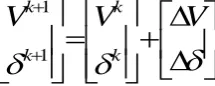
LOW

As all power flow calculations are done using iterative numerical methods using load flow studies. In this paper, the MATLAB simulation that is used to find the solutions to the test system power flow is based on the Newton-Raphson method in polar formulation. For power flow applications, variables P and Q are given, and Vand δ are to be calculated. To obtain final values of the V and δ vectors, first, an initial set of estimated values for the values of V and δ are assumed with one bus voltage and angle kept constant – the slack bus. The initial estimates are then used to compute the variation of the variables results from the initial iteration, ∆V and ∆ δ. The variations ∆V & ∆ δ are then used to make the next estimate.











































 



V

k k

1 1

The vectors Vk+1 and δk+1 are values for the k+1th iteration, Vk and δk are results from the previous kth iteration. The real and reactive power at any bus p for node p & q are given by [10].

Pp =Real Vp*

Ypq

Vq

n

q



(4)

= 1

|

cos(

)

q

p

pq

Ypq

Vq

Vp

n q













=|VpVpYpp|cos( )+

|

cos

)

1

q

p

pq

Ypq

Vq

Vp

n p q q











  And

Qp = Img Vp*

Ypq

Vq

n

q



1

=

|

sin

(

)

1

q

p

pq

Ypq

Vq

Vp

n q













=|VpVqYpq|sin + _| _|_sin( ₎

1 q p pq Ypq Vq Vp n p q q





 



 

For p=1,…..n-1 as the nthbus is a slack bus. Now the linear equation in the polar form becomes:











































|

4

3

2

1 V

J

Q

P



Where J1, J2,J3 and J4 are the elements of jacobian matrix which can be calculated from above eqns as follows.The variations vectors∆V and∆ δ are computed by using the following equation :

















V

= - 1

k p k k p J Q

P

                  

The matrix [Jk] is called the system Jacobian matrix, that can be divided into 4 quadrants as follows:

 

J

=





































































|

Vp

Qp

p

Qp

Vp

Pp

p

Pp



And elements for each quadrant are computed as follows: a.)

_













p

Pp



is an n ×n matrix. The diagonal

elements are calculated as follows:















p

Pp



= -



  n p q q 1

| Vp VqYpq| sin ( + − )

b)

|

|Vp

Pp



is an n ×n matrix. The diagonal elements are calculated as follows:

|

|Vp

Pp



= 2 |Vp Ypp| cos +



  n p q q 1

| Vq Ypq| Cos

( + − ) c.)

_













p

Qp



is an n x n matrix. The diagonal elements

are calculated as follows:

p

Qp





=



  n p q q 1

VpVqYpq|Cos ( + − )

d.)

_













|

| Vp

Qp

is an n ×n matrix. The diagonal elements are calculated as follows:

|

|Vp

Qp



= 2 | VpYpp| sin +



  n p q q 1

| VqYpq | sin

( + − )

Once the components described above are set in place, the iterative process is started. The initial estimate of the

solutions are entered as and then used to calculate

the first variation vector The second iteration’s estimates are thus obtained and then used to calculate the next estimates. The process is repeated until the solution converges. The solution is generally considered converged once the variation vector becomes small enough to fall within a tolerance value. Also, the initial values entered for the slack bus is one per-unit in magnitude and zero degrees in phase shift. The power loss is then given by; Ploss=Re[





n

p 1



Vp

(





n

p 1



Vp

Ypq)*] =





n

q 1



 n

q 1 VpVq YpqCos ( δp– δq– pq)

V. S

IMULATION

R

ESULTS OF

L

OSSES AT

B

US

2

The diagram for a two-bus system is shown in Figure 3 below where the electrical properties needed to complete a load-flow calculation for power loss in the transmission line are given below.

Fig.3. Single-Line Diagram of a Two-Bus, Two-Load Power System with Known Load and Known Transmission Line Data (Each bus can be the Slack Bus)

Specifications of the two-bus test system

(5)

 Conductor size =95mm2, Diameter of String=2.52mm, Number of strings=19

• Transmission Line Resistance = 5 km * 0.340589 Ohms/conductor/km (at 500C) * 3 conductors

 Reactance = 5 km * 0.356424

Ohms/cond./km(Single circuit)*3conductors

Figure 4 shows the load profile of each load at 2 bus varies with time and has a different pattern over a period of 24 hours.

Fig.4. Load Demands for the Two-Bus Power System The two bus system has been used to be a source for a simple load-flow calculation program written in MATLAB to determine the losses for the transmission line. The incurred Active & Reactive Power losses in Transmission lines without NTL is shown in Figure 5 below.

Fig.5. Active Power Losses & Reactive Power Losses at Bus 2

In this case bus 1 is used as the slack bus, the maximum active power loss in the transmission line is around 380

watts at 15 hrs and that of reactive power loss is 400 VARs at the same time without addition of NTL Load.

The extra load may be simulated in a simplistic way by adding a profile of demands to the bus 2 load in the form of adding KVA values to the original demand and reducing the total power factors by subtracting a power factor “contribution” for each value of added load. The power factor (pf) contributions chosen here were negative because the NTL load is assumed to be Inductive, i.e., motors or light fixtures. The profile of the added NTL, the total load at bus 2 are shown in Figure 6.

Fig.6. NTL Contribution to Industrial Load at Bus 2 The simulation is run with bus 1 as the slack bus. The NTL pf contribution is negative at all times because the NTL load is assumed to be inductive. After the simulation was completed and evaluated, some notable results were evident. The Active & Reactive power losses along with NTL in transmission line are shown in Figure7.

Fig.7. Active Power Losses Reactive Power Losses with NTL at Bus 2

In this case where bus 1 is used as the slack bus, the maximum active power loss in the transmission line is around 400 watts at 15 hrs and that of reactive power loss

0 50 100 150 200 250 300 350

1 3 5 7 9 11 13 15 17 19 21 23

0 5 10 15 20 25

0 100 200 300 400

Time(Hrs)

A

ct

iv

e

P

ow

er

L

os

s

(W

at

ts

) REGULAR POWER LOSS IN WATTs

0 5 10 15 20 25

0 100 200 300 400

Time(Hrs)

R

ea

ct

iv

e

Po

w

er

L

os

s

(V

A

R

s) REGULAR REACTIVE POWER LOSS IN VARs

0 50 100 150 200 250 300 350

1 3 5 7 9 11 13 15 17 19 21 23

0 5 10 15 20 25

0 100 200 300 400 500

Time(Hrs)

Ac

tiv

e P

ow

er

Lo

ss

wi

th

NT

L

NTL POWER LOSS IN WATTs

0 5 10 15 20 25

0 100 200 300 400 500

Time(Hrs)

Re

ac

tiv

e P

ow

er

Lo

ss

w

ith

N

TL

(6)

is 420 VARs at the same time because NTL is added at bus 2.

VI. C

ONCLUSION

As NTL cannot be computed & measured easily, but it can be estimated from preliminary results, i.e. the result of technical losses are first computed and subtracted from the total losses, with the balance as NTL. The technical losses are calculated using appropriate load flow studies using Matlab Software. The low voltage distribution systems of 11KV are not as thoroughly measured because of the costs of the added metering. This is the reason that power flow solutions are used to estimate the states at various points in the system. The conclusion is that if data about NTL loads is available to analyst only then the measurement of NTL and its effects on electrical power systems can be determined. The data is to include, either the NTL load power consumption profile comparable to the legitimate loads, being analyzed at the same time, as well as the NTL power factor, or power factor contribution. In this paper, I have considered a two-bus system with loads at both buses and either of one bus can be selected as a “slack bus” with constant voltage and phase angle necessary for analysis of the system. The extra load was simulated in a simplistic way by adding a profile of demands to the bus 2 load in the form of adding KVA values to the original demand and reducing the total power factors by subtracting a power factor “contribution” for each value of added load. The pf contributions chosen here were negative because the NTL load is assumed to be Inductive. The load profile of each load varies with time and has a different pattern over a period of 24 hours. To make the test loads more realistic they are represented as two sets of power demands with different operation schedules comparable to residential and industrial area. In the case where bus 1 is used as the slack bus, the maximum active power loss in the transmission line is around 380 watts at 15 hrs and that of reactive power loss is 400 VARs at the same time. As NTL is added at node 2 and node 1 is used as the slack node, the maximum active power loss in the transmission line is around 400 watts at 15 hrs and that of reactive power loss is 420 VARs at the same time. Thus, it may be concluded that as NTL load is added to the system, total losses will increase which further creates costs for SEBs in the form of lost revenues.

R

EFERENCES

[1] “Electricity Scenario in India”, A report issued by Central Electric Authority, Ministry of Power, Government of India, 2008.

[2] J.P. Navani, N.K Sharma, Sonal Sapra, "Technical and Non-Technical Losses in Power System and Its Economic Consequence in Indian Economy" International Journal of Electronics and Computer Science Engineering, vol. 1, pp.757-761, 2011.

[3] Yoginder Alagh, “Transmission and Distribution of Electricity in India Regulation, Investment and Efficiency”, IRMA, 2010 [4] V. Kumar and A. Chandra, “Role of Geographical Information

Systems in distribution management”, Central Electricity Authority, New Delhi. March 2010.

[5] Nizar A.H.; Dong Z.Y.; Jalaluddin, M.:, Raffles, M.J.;” Load Profiling Method in Detecting NTL Activities in A power

Utility,”, IEEE International Conference on Power System and Energy, Vol . 2, PP. 82-87, Nov. 2006.

[6] Dong Z.Y.; Zhao, J.H.,” Load Profiling and Data Mining technique in Electricity Deregulated Market,”, power Engineering Society General Meeting, IEEE Vol . 2, PP.7-9, 2006.

[7] IE Davidson and A Odubiyi, “Technical loss computation and economic dispatch model forT&D systems in deregulated ESI”, Power Engineering Journal, p 55, 2002.

[8] DC Neethling and RK Dutkiewicz,”International and regional energy policy development, focusing on end use of energy”, Enerconomy, p 93, 1993.

[9] N.Krishnaswamy,”A holistic approach to practical techniques to analysis and reduce technical losses on Eskom power networks using the principles of management of technologies”, Management of technology, Technology leadership program, p 28-33, 2000.

[10] L.P.Singh, “Advanced Power System Analysis & Dynamics,” New Age International Publishers, India,

A

UTHOR

’

S

P

ROFILE

(A) Deepak Madan

is postgraduate student in Electrical & Electronics Engineering (power electronics & drives) at Kurukshetra university, Kurukshetra, Haryana, India. He received his B.Tech degree in Electrical Engineering from Punjab Technical University in 2010. E-mail Id : [email protected]

(B) Meenakshi Dhakla

received her B.E. degree in Bio-Medical Engineering from Deenbandhu Chhotu Ram University of Science and Technology, Murthal in 2009, the M.Tech. degree in Instrumentation and Control Engineering from the same University in

2011. Presently, she is an assistant professor, with Department of Electrical and Electronics Engineering, Doon Valley Institute of Engineering and Technology, Karnal.

E-mail Id : [email protected]

(C) Balvinder Dhull