doi:10.5194/gmd-10-1091-2017
© Author(s) 2017. CC Attribution 3.0 License.
Development of a probabilistic ocean modelling system based on
NEMO 3.5: application at eddying resolution
Laurent Bessières1, Stéphanie Leroux2, Jean-Michel Brankart2, Jean-Marc Molines2, Marie-Pierre Moine1, Pierre-Antoine Bouttier2, Thierry Penduff2, Laurent Terray1, Bernard Barnier2, and Guillaume Sérazin1,2 1CNRS/CERFACS, CECI UMR 5318, Toulouse, France
2Univ. Grenoble Alpes, CNRS, IRD, IGE, 38000 Grenoble, France
Correspondence to:Laurent Bessières ([email protected]) Received: 5 July 2016 – Discussion started: 19 September 2016
Revised: 16 December 2016 – Accepted: 4 January 2017 – Published: 10 March 2017
Abstract.This paper presents the technical implementation of a new, probabilistic version of the NEMO ocean–sea-ice modelling system. Ensemble simulations with N members running simultaneously within a single executable, and in-teracting mutually if needed, are made possible through an enhanced message-passing interface (MPI) strategy includ-ing a double parallelization in the spatial and ensemble di-mensions. An example application is then given to illus-trate the implementation, performances, and potential use of this novel probabilistic modelling tool. A large ensemble of 50 global ocean–sea-ice hindcasts has been performed over the period 1960–2015 at eddy-permitting resolution (1/4◦) for the OCCIPUT (oceanic chaos – impacts, structure, pre-dictability) project. This application aims to simultaneously simulate the intrinsic/chaotic and the atmospherically forced contributions to the ocean variability, from mesoscale tur-bulence to interannual-to-multidecadal timescales. Such an ensemble indeed provides a unique way to disentangle and study both contributions, as the forced variability may be es-timated through the ensemble mean, and the intrinsic chaotic variability may be estimated through the ensemble spread.
1 Introduction
Probabilistic approaches, based on large ensemble simula-tions, have been helpful in many branches of Earth-system modelling sciences to tackle the difficulties inherent to the complex and chaotic nature of the dynamical systems at play. In oceanography, ensemble simulations have first been in-troduced for data assimilation purposes, in order to
explic-itly simulate and, given observational data, reduce the uncer-tainties associated with, for example, model dynamics, nu-merical formulation, initial states, atmospheric forcing (e.g. Evensen, 1994; Lermusiaux, 2006). This type of probabilistic approach is also used to accurately assess ocean model sim-ulations against observations (e.g. Candille and Talagrand, 2005), or to anticipate on the design of satellite observational missions (e.g. Ubelmann et al., 2009).
Performing ensemble simulations can be seen as a natu-ral way to take into account the internal variability inherent to any chaotic and turbulent system, by sampling a range of possible trajectories of this system (independent and iden-tically distributed). For example, long-term climate projec-tions, or short-term weather forecasts, rely on large ensem-bles of atmosphere–ice–ocean coupled model simulations to simulate the probabilistic response of the climate system to various external forcing scenarios, or to perturbed initial con-ditions, respectively (e.g. Palmer, 2006; Kay et al., 2015; Deser et al., 2016).
Grégorio et al., 2015; Sérazin et al., 2015). The evolution of this chaotic ocean variability under repeated climatological atmospheric forcing is sensitive to initial states. This suggests that turbulent oceanic hindcasts driven by the full range of at-mospheric scales (e.g. atat-mospheric reanalyses) are likely to be sensitive to initial states as well, and their simulated vari-ability should be interpreted as a combination of the atmo-spherically forced and the intrinsic/chaotic variability.
On the other hand, NEMO climatological simulations at ∼2◦resolution (in the laminar non-eddying regime) driven by a repeated climatological atmospheric forcing are almost devoid of intrinsic variability (Penduff et al., 2011; Grégo-rio et al., 2015). Because∼1/4◦-resolution OGCMs are now progressively replacing their laminar counterparts at ∼1– 2◦resolution used in previous CMIP-type long-term climate projections (e.g. HighResMIP, Haarsma et al., 2016), it be-comes crucial to better understand and characterize the re-spective features of the intrinsic and atmospherically driven parts of the ocean variability, and their potential impact on climate-relevant indices.
Simulating, separating, and comparing these two compo-nents of the oceanic variability requires an ensemble of tur-bulent ocean hindcasts, driven by the same atmospheric forc-ing, and started from perturbed initial conditions. The high computational cost of performing such ensembles at global or basin scale explains why only a small number of stud-ies have carried out this type of approach until now, and with small ensemble sizes (e.g. Combes and Lorenzo, 2007; Hirschi et al., 2013).
Building on the results obtained from climatological simu-lations, the ongoing OCCIPUT project (Penduff et al., 2014) aims to better characterize the chaotic low-frequency intrin-sic variability (LFIV) of the ocean under a fully varying at-mospheric forcing, from a large (50-member) ensemble of global ocean–sea-ice hindcasts at 1/4◦ resolution over the last 56 years (1960–2015). The intrinsic and the atmospheri-cally forced parts of the ocean variability are thus simulated simultaneously under a fully varying realistic atmosphere, and may be estimated from the ensemble spread and the en-semble mean, respectively. This strategy also allows investi-gation into the extent to which the full atmospheric variabil-ity may excite, modulate, damp, or pace intrinsic modes of oceanic variability that were identified from climatological simulations. OCCIPUT mainly focuses on the interannual-to-decadal variability of ocean quantities having a potential impact on the climate system, such as sea surface tempera-ture (SST), meridional overturning circulation (MOC), and upper ocean heat content (OHC).
This paper presents the technical implementation of the new, fully probabilistic version of the NEMO modelling sys-tem required for this project. It stands at the interface be-tween scientific purposes and new technical developments implemented in the model. The OCCIPUT project is psented here as an application, to illustrate the system re-quirements and numerical performances. The mathematical
background supporting our probabilistic approach is detailed in Sect. 2. Section 3 describes the new technical develop-ments introduced in NEMO to simultaneously run multiple members from a single executable (allowing the online com-putation of ensemble statistics), with a flexible input–output strategy. Section 4 presents the implementation of this prob-abilistic model to perform regional and global 1/4◦ ensem-bles, both performed in the context of OCCIPUT. The strat-egy chosen to trigger the growth of the ensemble spread, and the numerical performances of both implementations are also discussed. Section 5 finally presents some preliminary results from OCCIPUT to further illustrate potential scientific appli-cations of this probabilistic approach. A summary and some concluding remarks are given in Sect. 6.
2 From deterministic to probabilistic ocean modelling: mathematical background
The classical, deterministic ocean model formulation can be written as follows:
dx=M(x, t )dt, (1)
wherex=(x1, x2, . . ., xN)is the model state vector,tis time,
andMis the model operator, containing the expression of
the tendency for every model state variable. An explicit time dependence is included in the model operator since the ten-dencies depend on the time-varying atmospheric forcing.
Computing a solution to Eq. (1) requires the specification of the initial condition att=0, from which the future evolu-tion of the system is fully determined. OCCIPUT investigates how perturbations in initial conditions evolve and finally af-fect the statistics of climate-relevant quantities. This problem may be addressed probabilistically by solving the Liouville equation:
∂p(x, t )
∂t = −
N X
k=1
∂ ∂xk
M(x, t )p(x, t ), (2)
t x
p(x,t )0 p(x,t )1 p(x,t )2
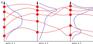
Figure 1.Schematic of an ensemble simulation (red trajectories),
as an approximation to the simulation of an evolving probability distribution (in blue).
In addition to uncertainties in the initial condition, it is sometimes useful to assume that the model dynamics them-selves are uncertain. This leads to a non-deterministic ocean model formulation, in which model uncertainties are de-scribed by stochastic processes. One possibility is, for in-stance, to modify Eq. (1) as follows.
dx=M(x, t )dt+6(x, t )dWt (3)
In this equation,Wtis anM-dimensional standard Wiener
process, and6(x, t )is anN×Mmatrix, describing the in-fluence of these processes on the model tendencies. Equa-tion (3) does not include all possible ways of introducing a stochastic parameterization in a dynamical model, but it is sufficient to include the implementation that is described in this paper (in particular, to include the use of space-correlated or time-space-correlated autoregressive processes by ex-panding the definition of x in Eq. 3). With this additional
stochastic term, Liouville equation transforms to Fokker– Planck equation:
∂p(x, t )
∂t = −
N X
k=1
∂
∂xk
M(x, t )p(x, t ) (4)
+ 12
N X
k=1 N X
l=1
∂2 ∂xk∂xl
Dkl(x, t )p(x, t )
,
whereDkl(x, t )=PMp=16kp(x, t )6lp(x, t ). The probability
distributionp(x, t )is thus affected by the stochastic diffu-sion tensorD(x, t )during its advection in the phase space by local model tendencies.
However, since Eqs. (2) and (4) are partial differential equations in anN dimensional space, they generally cannot be solved explicitly for large size systems. Only an approxi-mate description ofp(x, t )can be obtained in most practical situations. A common solution is to reduce the description of p(x, t )to a moderate size sample, which can be viewed as a Monte Carlo approximation to Eqs. (2) and (4). This ap-proach is illustrated in Fig. 1. The computation is initialized by a sample of the initial probability distributionp(x, t0)(on the left in the figure), and each member of the sample is used as a different initial condition to Eqs. (1) and (3). The classi-cal model operator can then be used to produce an ensemble
of model simulations (red trajectories in the figures), which provide a sample of the probability distribution at any future time, e.g.p(x, t1), orp(x, t2).
This Monte Carlo approach is very general and can be also applied to any kind of stochastic parameterization (not only the particular case described by Eq. 3). It was first applied to ocean models in the framework of the ensemble Kalman filter (Evensen, 1994) to solve ocean data assimilation problems.
In summary, Eq. (1) describes the problem that is classi-cally solved by the NEMO model; Eq. (3) is a modification of this problem with stochastic perturbations of the model equations that explicitly simulate model uncertainties; in this paper, this problem is solved using an ensemble simula-tion, which provides identically distributed realizations from the probability distribution, and thus a way to compute any statistic of interest.
3 Performing ensemble simulations with NEMO The NEMO model (Nucleus for a European Model of the Ocean), described in Madec (2012), is used for oceano-graphic research, operational oceanography, seasonal fore-casts and climate studies. This system embeds various model components (see http://www.nemo-ocean.eu/), including a circulation model (OPA, Océan PArallélisé), a sea-ice model (LIM, Louvain-la-Neuve ice model), and ecosystem models with various levels of complexity. Every NEMO component solves partial differential equations discretized on a 3-D grid using finite-difference approximations. The purpose of this section is to present the technical developments introduced in our probabilistic NEMO version, and to make the connec-tion between these new developments and existing NEMO features.
3.1 Ensemble NEMO parallelization
The standard NEMO code is parallelized with MPI (message-passing interface) using a domain decomposition method. The model grid is divided in rectangular subdomains (i=1, . . ., n), so that the computations associated with each subdomain can be performed by a different processor of the computer. Spatial finite-difference operators require knowl-edge of the neighbouring grid points, so that the subdomains must overlap to allow the application of these operators on the discretized model field. Whenever needed, the overlap-ping regions of each subdomain must be updated using the computations made for the neighbouring subdomains. The NEMO code provides standard routines to perform this up-date. These routines use MPI to get the missing information from the other processors of the computer. This communica-tion between processors makes the conneccommunica-tion between sub-domains in the model grid.
00 00 11 11 00 00 11 11 00 00 11 11 00 00 11 11 00 00 11 11 00 00 11 11 00 00 11 11 00 00 11 11 00 00 11 11 00 00 11 11 00 00 11 11 00 00 11 11 00 00 11 11 00 00 11 11 00 00 11 11 00 00 11 11 00 00 11 11 00 00 11 11 00 00 11 11 00 00 00 11 11 11
1 2 3 n−1 n
S ubdomains
E nsemble members
1
m
m−1
2
O ne MPI communicator
O ne MPI communicator
for each subdomain
for each ensemble member
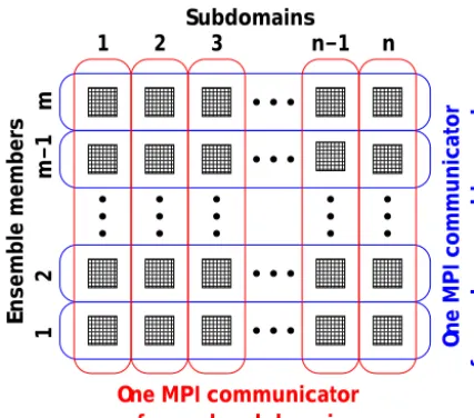
Figure 2. Schematic of the double parallelization introduced in
NEMO: each processor (black squares) is dedicated to the com-putations associated with one model subdomain and one ensem-ble member. There is one MPI communicator within each ensemensem-ble member (in blue) to allow communications between neighbouring subdomains as in the standard NEMO parallelization, and there is one MPI communicator within each model subdomain (in red) to allow communication between ensemble members (e.g. to compute ensemble statistics online if needed). The total number of proces-sors is thus equal to the product of the ensemble size by the number of subdomains (m×n).
processor is associated with a subdomain and knows which are its neighbours.
Ensemble simulations may be performed with NEMO by a direct generalization of the standard parallelization proce-dure described above. In other words, our ensemble simula-tions are performed from one single call to the NEMO ex-ecutable, simply using more processors to run all members in parallel. This technical option is both natural and unnat-ural. It is natural since an ensemble simulation provides an approximate description of the probability distribution; it is thus conceptually appealing to advance all members together in time. It is unnatural since independent ensemble members may be run separately (in parallel, or successively) using in-dependent calls to NEMO. However, the solution we propose is so straightforward that there is virtually no implementa-tion cost, and is more flexible since the ensemble members may be run independently, by groups of any size, or all to-gether. Furthermore, running all ensemble members together provides a new interesting capability: the characteristics of the probability distributionp(x, t )in Eq. (2) or (4) may be computed online, virtually at every time step of the ensem-ble simulation. This has been done using MPI to gather the required information from every member of the ensemble. These MPI communications make a natural connection be-tween ensemble members, as a sample of the probability dis-tributionp(x, t ).
In practice, this implementation option only requires that at the beginning of the NEMO simulation, one MPI commu-nicator is defined for each ensemble member, each one with as many processors as subdomains, so that each processor knows to which member it belongs, on which subdomain it is going to compute and what its neighbours are. Inside each of these communicators, each ensemble member may be run in-dependently from the other members, without changing any-thing else in the NEMO code. However, all members are ob-viously not supposed to behave exactly the same: the index of the ensemble member must have some influence on the simu-lation. This influence may be in the name of the files defining the initial condition, parameters or forcing, or in the seeding of the random number generator (if a random forcing is ap-plied, as in Eq. 3). The index of the ensemble member must also be used to modify the name of all output files, so that the output of different members is saved in different files. As it appears, this implementation of ensemble simulations does not require much coding effort (a few tens of lines in NEMO, partly because most of the basic material was already avail-able in the original code). More technical details about this can be found in Sect. 7.
In summary, the NEMO ensemble system relies on a dou-ble parallelization, over model subdomains and over ensem-ble members, as illustrated in Fig. 2. In this algorithm, en-semble simulations are thus intricately linked to MPI paral-lelization. There is no explicit loop over the ensemble mem-bers; this loop is done implicitly through MPI; running more ensemble members means either using more processors or using less processors for each member.
3.2 Online ensemble diagnostics
As mentioned above, one important novelty offered by the ensemble NEMO parallelization is the ability to compute on-line any feature of the probability distributionp(x, t ). This can be done within additional MPI communicators connect-ing all ensemble members for each model subdomain (in red in Fig. 2). MPI sums in these communicators are for instance immediately sufficient to estimate the following:
– the mean of the distribution:
µk= Z
xkp(x, t )dx (5)
∼eµk=
1 m
m X
j=1
xk(j ),
wherexk is one of the model state variables,xk(j )is this
variable simulated in memberj,µk is the mean of the
distribution for this variable, andeµk is the estimate of
all processors of the ensemble communicators (in red in Fig. 2). The same remark also applies to the sums in the following equations.
– the variance of the distribution: σk2=
Z
(xk−µk)2p(x, t )dx
∼eσ
2
k =
1 m−1
m X
j=1
xk(j )−eµk 2
,
whereσk2is the variance of the distribution for variable xk andeσ
2
k is the estimate obtained from the ensemble.
The ensemble standard deviation is simply the square root ofeσ
2
k.
– Ensemble covariance between two variables at the same model grid point:
γkl= Z
(xk−µk) (xl−µl) p(x, t )dx
∼eγkl=
1 m−1
m X
j=1
xk(j )−eµk x(j )l −eµl
,
whereγklis the covariance between variablesxkandxl,
andeγklis the estimate obtained from the ensemble.
This is directly generalizable to the computation of higher-order moments (skewness, kurtosis), which is then reduced to MPI sums in the ensemble communicators. Moreover, sim-ple MPI algorithms can also be designed to compute many other probabilistic diagnostics online, such as the rank of each member in the ensemble, and from there, estimates of quantiles of the probability distribution. Specific applications of this feature are discussed in Sect. 5.
This online estimation of the probability distribution, via the computation of ensemble statistics, opens another inter-esting new capability: the solution of the model equations may now depend on ensemble statistics, available at each time step if needed. For instance, it may be interesting to lax the modelled forced variability towards reference (e.g. re-analysed or climatological) fields, with no explicit damping of the intrinsic variability: the nudging term would involve the current ensemble mean and be applied identically to all members at the next time step, resulting in a simple “transla-tion” of the entire ensemble distribution toward the reference field.
Other applications, such as ensemble data assimilation, may also require an online control of the ensemble spread, which is hereby made possible within NEMO.
3.3 Connection with NEMO stochastic parameterizations
Ensemble simulations are directly connected to stochas-tic parameterizations (as introduced in Eq. 3). In NEMO,
stochastic parameterizations have recently been imple-mented to explicitly simulate the effect of uncertainties in the model (Brankart et al., 2015). In practice, this is done by generating maps of autoregressive processes, which can be used to introduce perturbations in any component of the model. In Brankart et al. (2015), examples are provided to illustrate the effect of these perturbations in the circulation model, in the ecosystem model and in the sea ice model. For instance, a stochastic parameterization was introduced in the circulation model to simulate the effect of unresolved scales in the computation of the large-scale density gradient, as a result of the nonlinearity of the sea water equation of state (Brankart, 2013). This particular stochastic parameterization is switched on during one year in order to initiate the disper-sion of the OCCIPUT ensemble simulations started from a single initial condition (see Sect. 4).
3.5 Connection with the NEMO observation operator and model assessment metrics
Another important benefit of the probabilistic approach is to consolidate and objectivate statistical comparisons between actual observations and model-derived ensemble synthetic observations. Probabilistic assessment metrics are commonly used in the atmospheric community (e.g. Toth et al., 2003) but are quite new in oceanography. Briefly speaking, these methods generally quantify two attributes of an ensemble simulation: thereliabilityand theresolution. An ensemble is reliable if the simulated probabilities are statistically consis-tent with the observed frequencies. The ensemble resolution is related to the system ability to discriminate between dis-tinct observed situations. If the ensemble is reliable, the res-olution is directly related to the information content (or the spread) of the probability distribution. A popular measure of these two attributes is, for instance, provided by the contin-uous rank probability score (CRPS), which is based on the square difference between a cumulative distribution function (CDF) as provided by the ensemble simulation and the corre-sponding CDF of the observations (Candille and Talagrand, 2005).
In OCCIPUT, such probabilistic scores will be computed from real observations and from the ensemble synthetic ob-servations (along-track Jason-2 altimeter data and ENACT– ENSEMBLES temperature and salinity profile data) gen-erated online using the existing NEMO observation opera-tor (NEMO-OBS module). NEMO-OBS is used exactly as in standard NEMO within each member of the ensemble, thereby providing an ensemble of model equivalents for each observation rather than a single value. Probabilistic metrics (i.e. CRPS score) will then be computed to assess the relia-bility and resolution of the OCCIPUT simulations.
3.6 Connection with NEMO I/O strategy
Our implementation of ensemble NEMO using enhanced parallelization is technically not independent from the NEMO I/O strategy. Indeed, in NEMO, the input and output of data is managed by an external server (XIOS, for XML IO Server), which is run on a set of additional processors (not used by NEMO). The behaviour of this server is controlled by an XML file, which governs the interaction between XIOS and NEMO, and which defines the characteristics of input and output data: model fields, domains, grid, I/O frequen-cies, time averaging for outputs, etc. To exchange data with disk files, every NEMO processor makes a request to the XIOS servers, consistently with the definitions included in the XML file. In this operation, the XIOS servers buffer data in memory, with the decisive advantage of not interrupting NEMO computations with the reading or writing in disk files. One peculiarity of this buffering is that each XIOS server reads and writes one stripe of the global model domain (along the second model dimension), and thus exchanges data with
processors corresponding to several model subdomains. To optimize the system, it is obviously important that the num-ber of XIOS servers (and thus the size of these stripes) be correctly dimensioned according to the amount of I/O data, which may heavily depend on the model configuration and on the definition of the model outputs.
To use XIOS with our implementation of ensemble NEMO for OCCIPUT, we thus had to take care of the two following issues. First, different ensemble members must write differ-ent files. This problem could be solved because XIOS was already designed to work with a coupled model, and can thus deal with multiple contexts: i.e. one for each of the coupled model components. It was thus directly possible to define one context for each ensemble member, just as if they were dif-ferent components of a coupled model. Second, in ensemble simulations, the amount of output data is proportional to the ensemble size, so that the number of XIOS servers must be increased accordingly, albeit with some care, because the size of the data stripe that is processed by each server should not be reduced too much.
4 Example of application: the OCCIPUT project The implementation of this ensemble configuration of NEMO was motivated to a large extent by the scientific ob-jectives of the OCCIPUT project, described in the introduc-tion. In this section, we present two ensemble simulations, E-NATL025 and E-ORCA025, performed in the context of this project. We focus on the model set-up, the integration strategy, and the numerical performances of the system, fol-lowed by a few illustrative preliminary results in Sect. 5. 4.1 Regional and global configurations
cal simulation used in Penduff et al. (2011), Grégorio et al. (2015), and Sérazin et al. (2015) to study various imprints of the LFIV under seasonal atmospheric forcing.
4.2 Integration and stochastic perturbation strategies A one-member spin-up simulation is first performed for each ensemble. For the regional ensemble (E-NATL025), it is performed from 1973 (cold start) to 1992, forced with DFS.5.2 atmospheric conditions (Dussin et al., 2016). For the global ensemble (E-ORCA025), the spin-up strategy has to be adapted to match the OCCIPUT objective to perform the ensemble hindcast over the longest period available in the atmospheric forcing DFS5.2 (i.e. 1960–2015). The one-member spin-up simulation is thus performed as follows: (1) it is first forced by the standard DFS5.2 atmospheric forcing from 1 January 1958 (cold start) to 31 Decem-ber 1976; (2) this simulation is continued over January 1977 with a modified forcing function that linearly interpolates be-tween 1 January 1977 and 31 January 1958; (3) the stan-dard DFS5.2 forcing is applied again normally from 1 Febru-ary 1958 to the end of 1959. This 21-year spin-up (1958– 1977, then 1958–1959) thus includes a smooth artificial tran-sition from January 1977 back to January 1958. This choice was made as a compromise to maximize the duration of the single-member spin-up simulation and of the subsequent en-semble hindcast, while minimizing the perturbation in the forcing during the transition, since 1977 was found to be a reasonable analogue of 1958 in terms of key climate indices (El Niño Southern Oscillation, North Atlantic Oscillation, and Southern Annular Mode).
The N members of both ensemble simulations (i.e.N= 10 for E-NATL025 andN=50 for E-ORCA025) are started at the end of the single-member spin-up; a weak stochastic perturbation in the density equation, as described by Eq. (3) and in Sect. 3.3 (see also Brankart et al., 2015) is then ac-tivated within each member. This stochastic perturbation is only applied for 1 year to seed the ensemble dispersion (dur-ing 1993 for E-NATL025, dur(dur-ing 1960 for E-ORCA025). It is then switched off throughout the rest of the ensemble sim-ulations. Once the stochastic perturbation is stopped, theN members are thus integrated from slightly perturbed initial conditions (i.e. 19 more years for E-NATL025 and 55 more years for E-ORCA025), but forced by the exact same atmo-spheric conditions (DFS5.2, Dussin et al., 2016). The code is parallelized with the double-parallelization technique de-scribed in Sect. 3.1 so that the N members are integrated simultaneously through one single executable.
4.3 Performance of the NEMO ensemble system in OCCIPUT configurations
The regional ensemble (E-NATL025) was performed to test the system implementation and to calibrate the global configuration. The global ensemble simulation
E-ORCA025 represents, in total, 2821 cumulated years of simulation (56 years×50 members+21 years of one-member spin-up) over 110 million grid points (longi-tude×latitude×depth=1442×1021×75). As confirmed thereafter in Fig. 3, integrating such a system within one ex-ecutable with reasonable wall-clock time, and managing its outputs lies beyond national or regional European centres computational capabilities (i.e. Tier-1 systems), requiring systems that can provide European top capabilities, which are beyond the Petaflops level (i.e. Tier-0 systems).
All simulations were performed between 2014 and 2016 on the French Tier-0 Curie supercomputer, supported by PRACE (Partnership for Advanced Computing in Europe) and GENCI (Grand Equipement National de Calcul Intensif, French representative in PRACE) grants (19.106HCPU, see details below). Curie is a Bull system (BullX series designed for extreme computing) based on Intel processors. The archi-tecture used for the simulations is the one of the “Curie thin nodes” configuration (Curie-TN), which is mainly targeted at MPI parallel codes and includes more than 80 000 Intel Sandy Bridge computing cores (Peak frequency per core: 2.7 GHz) gathered in 16-core nodes of 64 GB of memory.
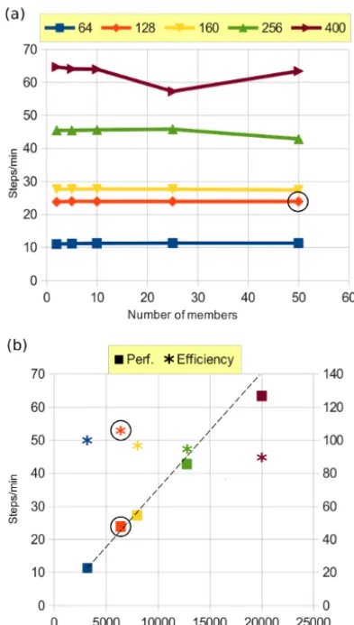
Preliminary tests showed that the one-member ORCA025 configuration has a good scalability up to 400 cores on Curie-TN (not shown). In order to test the ensemble global config-uration on Curie-TN, short 180-step experiments were run, disregarding the first and last steps (which correspond to reading and writing steps, respectively, that are performed only once during production jobs). The performance of the system was measured in steps per minute by analysing the 160 steps in between (steps 10 to 170). Figure 3a shows this measure of the system performance (in steps min−1) as a function of the number of members, for different domain de-compositions (64, 128, 160, 256, and 400 cores member−1). It appears that the performance is independent of the ensem-ble size for domain decomposition up to 160 domains per member. When more than 160 domains per member are used, the performance starts to decrease for increasing ensemble size, from 25 members (10) for the decomposition with 256 (400) domains per member. Fluctuations in steps per minute may appear (see the performance for the decomposition with 400 domains per member and 25 members in Fig. 3a), de-pending on machine load and file system stability (the perfor-mance of this specific point has not been reassessed for CPU cost reasons). The scalability of the global ensemble config-uration E-ORCA025, as aimed for in OCCIPUT (N=50), is shown in Fig. 3b: the efficiency is measured as the ratio of the observed speedup to the theoretical speedup, relative to the smallest domain decomposition tested, i.e. with 3200 cores (50×64). The efficiency is remarkably good and re-mains around 90 % for 20 000 used cores.
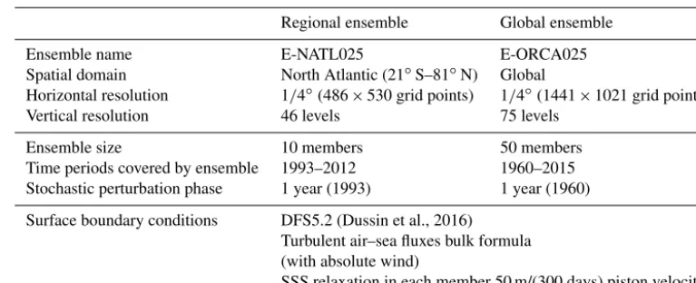
Table 1.Main characteristics of the NEMO 3.5 set-up used for the regional and global OCCIPUT ensembles.
Regional ensemble Global ensemble
Ensemble name E-NATL025 E-ORCA025
Spatial domain North Atlantic (21◦S–81◦N) Global
Horizontal resolution 1/4◦(486×530 grid points) 1/4◦(1441×1021 grid points)
Vertical resolution 46 levels 75 levels
Ensemble size 10 members 50 members
Time periods covered by ensemble 1993–2012 1960–2015 Stochastic perturbation phase 1 year (1993) 1 year (1960) Surface boundary conditions DFS5.2 (Dussin et al., 2016)
Turbulent air–sea fluxes bulk formula (with absolute wind)
SSS relaxation in each member 50 m/(300 days) piston velocity
red line in Fig. 3) so that 50×128=6400 cores are used for the ensemble NEMO system.
In order to optimize and to make the I/O data flux man-agement flexible, 40 XIOS servers have been run as inde-pendent MPI tasks in detached mode, allowing the overlap of I/O operations with computations. Compared to the 10-member regional case, the 50-10-member global case required a larger XIOS buffer size. For this reason, each of the 40 XIOS instances was run on a dedicated and exclusive Curie-TN, allowing each server to use the entire memory available on each 16-core node (i.e. 64 GB); the 40 XIOS servers thus used 16×40=640 cores in total. The integration of the 50-member global E-ORCA025 ensemble therefore required the use of 6400+(40×16)=7040 cores.
XIOS makes use of parallel file system capabilities via the Netcdf4-HDF5 format, which allows both online data com-pression and parallel I/O. Therefore, XIOS is used in “mul-tiple file” mode where each XIOS instance writes a file for one stripe of the global domain, yielding 40 files times 50 members for each variable and each time. At the end of each job, the 40 stripes are recombined on-the-fly into global files. Preliminary tests have shown that the 50-member E-ORCA025 global configuration performs about 20 steps min−1, including actual I/O fluxes and addi-tional operations (e.g. production of ensemble synthetic observations). Since the numerical stability of this global setup requires a model time step of 720 s, about 2 million time steps, 85 days of elapse time, and about 14.4 million core hours were needed in theory to perform the 56-year OCCIPUT ensemble simulation. The final CPU cost of the global ensemble experiment was about 19 million CPU hours, due to fluctuations in model efficiency, occasional problems on file systems which required the repetition of certain jobs, the need to decrease the model time step (increased high-frequency variance in the wind forcing data over the last decades), and the online computation of en-semble diagnostics (high-frequency enen-semble covariances, all terms of the heat content budget ensemble) over the last
decade. The cost of online ensemble diagnostics depends on the call frequency, number, and size of the concerned fields, on the architecture of the machine, and on the performance of communications. Our online ensemble diagnostics con-cerned a few two-dimensional fields at hourly to monthly frequencies, and had a negligible cost.
The final E-ORCA025 global database is saved in Netcdf4-HDF5 format (chunked and compressed, compres-sion ratio in italicsbelow). The primary dataset produced by the model consists of the following: monthly aver-ages for fully 3-D fields (56 years×12 months×50 mem-bers×2.8 GB×41.5 %=39 TB), 5-day averages for 16 2-D fields (56 years×50 members×6.8 GB×30 %=6 TB), the Jason-2 and ENACT–ENSEMBLES ensemble synthetic observations (5 TB), and hourly ensemble statistics for key variables (1 TB). One restart file per member and per year is also archived (about 35 TB after compression). We then computed a secondary dataset, consisting in 50-member yearly/decadal averages of the 3-D-fields (2 TB), ensem-ble deciles of monthly/yearly/decadal 3-D-fields (6 TB), and data associated with on-line monitoring (1 TB). The total out-put amounts to less than 100 TB and 100 000 inodes on the Curie-TN file system.
5 Preliminary results from the OCCIPUT application We now present some preliminary results from the regional and global OCCIPUT ensemble simulations described in Sect. 4.1, in order to illustrate the concepts and the techni-cal implementation presented above.
5.1 Probabilistic interpretation
tem-Figure 3. (a)Performance of the global ensemble configuration as a function of ensemble sizeN, for five domain decompositions: 64, 128, 160, 256, and 400 cores per member (coloured lines).(b) Per-formance in steps per minute and efficiency in % of the global en-semble configuration with 50 members. The dotted line represents the theoretical speedup. The number of cores corresponds here toN times the number of subdomains per member. Our final choice (50 members, 128 cores per member) is indicated with black circles.
perature given the identical atmospheric evolution that forces all members.
These temperature anomalies were computed by first re-moving the long-term non-linear trend of the time series de-rived from a local regression model (as in Grégorio et al., 2015). This detrending step acts as a non-linear high-pass temporal filter with negligible end-point effect also called local regression (LOESS) detrending (e.g. Cleveland et al., 1992; Cleveland and Loader, 1996), which successfully re-moves the unresolved imprints of very low-frequency vari-abilities (of forced or intrinsic origin), and possible non-linear model drifts. We focus here on the ocean variability that is fully resolved in the 20-year regional simulation out-put; we thus choose to remove the total long-term trend of each member individually prior to plotting and analysing the
ensemble statistics presented here. The mean seasonal cycle computed over the ensemble has also been removed from the monthly time series.
The ensemble-mean time series (hereafter E-mean, also notedfµkin Sect. 3) was then computed from these detrended
time series, and illustrates the temperature evolution com-mon to all members, i.e. forced by the atmospheric variabil-ity. The temporal standard deviation (hereafter Time-SD) of this ensemble mean thus provides an estimate of the atmo-spherically forced variability.
The dispersion of individual time series about the ensem-ble mean indicates the amount of intrinsic chaotic variabil-ity generated by the model. Its time-varying magnitude may be estimated by the ensemble standard deviation (hereafter E-SD, also notedσek in Sect. 3). Besides these low-order
sta-tistical moments, ensemble simulations actually provide an estimate of the full ensemble probability density function distribution (E-PDF) at any time, with an accuracy that in-creases with the number of members in the ensemble (see also Sect. 3.2).
5.2 Initialization and evolution of the ensemble spread Unlike in short-range ensemble forecast exercises, we do not seek here to maximize the growth rate of the initial disper-sion; we let the model feed the spread and control its evolu-tion following its physical laws.
Figure 4b and d confirm that the stochastic perturbation strategy (Sect. 4.2) successfully seeds an initial spread be-tween the ensemble members. The evolution and growth rate of the temperature E-SD depend on the geographical loca-tion: it grows faster in turbulent areas such as the Gulf Stream (Fig. 4b) and slower in less-turbulent areas like the subtrop-ical gyre (Fig. 4d). Note that the spread keeps growing af-ter the stochastic parameaf-terization has been switched off at the end of 1993, and tends to reach some leveled and satu-rated value after a few years. It is nevertheless still subject to clear modulations of its magnitude on timescales ranging from monthly to interannual. An additional 8-year experi-ment (not shown here) has confirmed that when the small stochastic perturbation is applied over the whole simulation instead of 1 year, the overall evolution, magnitude, and spa-tial patterns of E-SD, as well as the ensemble mean solution, remain unchanged. In other words, the stochastic parameter-ization seeds the spread during the initialparameter-ization period, but the subsequent evolution and magnitude of intrinsic variabil-ity is subsequently controlled by the model non-linearities, regardless of the initial stochastic seeding.
5.3 Spatial patterns of the ensemble spread
Figure 4.Ensemble statistics of the monthly temperature anomalies from the regional ensemble E-NATL025, at depth 93 m at two grid points:(a, b)in the Gulf Stream (42◦N, 56◦W) and(c, d)in the North Atlantic subtropical gyre (22◦N, 42◦W). Anomalies are shown after detrending and seasonal cycle removed (see text for details).(a)The individual trajectories with time of the 10 members appear in thin grey. E-mean is in thick yellow, the interval between quantiles Q1 (25 %) and Q3 (75 %) is filled in dark blue, and the interval E-mean±1 E-SD is filled in green.(b)E-SD (intrinsic variability, green shading) is compared to the Time-SD of E-mean (forced variability, thick yellow line). Also shown in(b)is the distribution of Time-SD for the 10 members: ensemble mean of the Time-SDs (solid grey), minimum and maximum (dashed grey), and mean±1 ensemble standard deviation (pale blue shading).
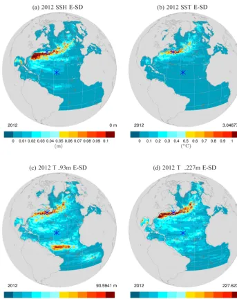
(i.e. 2012). These maps thus quantify the imprint of inter-annual intrinsic variability on these variables, and show that after 20 years of simulation, the ensemble spread has cas-caded from short (mesoscale-like) periods to long timescales. Annual E-SDs reach their maxima in eddy-active regions like the Gulf Stream (Fig. 5a) and the North Equatorial Countercurrent (Fig. 5c) where hydrodynamic instabilities
Figure 5.E-SD (shading) for year 2012 of the regional ensemble simulation E-NATL025, computed from annual means of(a)sea surface height (SSH),(b)sea surface temperature, and(c, d)temperature at depths 93 and 227 m, respectively. The contours show the corresponding E-mean fields. The blue symbols pinpoint the two grid points at which time series are shown in Fig. 4.
Comparing Fig. 5b, c, and d also illustrates that the en-semble spread of yearly temperature (i.e. its low-frequency intrinsic variability) peaks at subsurface (around the thermo-cline), and tends to decrease toward the surface in eddy-quiet regions.
This is expected from the design of these ensemble sim-ulations: each ensemble member is driven through bulk for-mulae by the same atmospheric forcing function, but turbu-lent air–sea heat fluxes differ somewhat among the ensemble because SSTs do so. This approach induces an implicit re-laxation of SST toward the same equivalent air temperature (Barnier et al., 1995) within each member, hence an artifi-cial damping of the SST spread. These experiments thus only
provide a conservative estimate of the SST intrinsic variabil-ity. Note that alternative forcing strategies may alleviate or remove this damping effect: ensemble mean air–sea fluxes may be computed online at each time step and applied iden-tically to all members (see Sect. 3.2). This alternative ap-proach is the subject of ongoing work and will be presented in a dedicated publication.
5.4 Magnitudes of forced and intrinsic variability
yellow line) is a proxy for the amount of the forced variabil-ity. It turns out to be dominated by the intrinsic variability (E-SD) at the Gulf Stream grid point. In less turbulent areas like the subtropical gyre, the intrinsic variability is still about 30–50 % of the forced part (Fig. 4d).
The E-SD can also be compared to the ensemble distri-bution of the Time-SDs of the N members (see caption of Fig. 4). By construction, the Time-SD of each member is due to both the forced (shared by all members) and the intrin-sic (unique to each member) variability. At the Gulf Stream grid point (Fig. 4b), these lines all lie above the Time-SD of E-mean, consistent with a high level of E-SD (i.e. intrinsic variability) contributing significantly to the total variability. At the subtropical gyre grid point, these lines fall much closer to E-mean since little intrinsic variability contributes to the total variability.
5.5 Toward probabilistic climate diagnostics
The variability of the atlantic meridional overturning circu-lation (AMOC) transport is of major influence on the climate system (e.g. Buckley and Marshall, 2016), and is being mon-itored at 26.5◦N since 2004 by the RAPID array (e.g. Johns et al., 2008). These observations are shown at monthly and interannual timescales as an orange line in Fig. 6, along with their simulated counterpart from E-ORCA025. They were computed in geopotential coordinates as in Zhang (2010) and Grégorio et al. (2015), and are shown after LOESS detrend-ing and after removdetrend-ing the mean seasonal cycle.
The simulated AMOC time series are in a good agreement with the observed AMOC variations at both monthly and an-nual timescales (Fig. 6a and c). The total (i.e. combination of forced and intrinsic) AMOC variability is computed as a Time-SD from the observed time series and from each en-semble member, and plotted in Fig. 6b and d as gray lines. At both timescales, the total AMOC variability simulated by E-ORCA025 lies below the observed variability, consistent with the fact that the model seems to miss a few observed peaks (e.g. 2005, 2009, and 2013 on the annual time se-ries). Figure 6b and d also highlight the substantial imprint of chaotic intrinsic variability on this climate-relevant oceanic index at both timescales: at interannual timescale, the AMOC intrinsic variability is weaker than the forced variability, but amounts to about 30 % of the latter. A more in-depth investi-gation of the relative proportion of intrinsic and forced vari-ability in the AMOC and of the variations of the intrinsic contribution with time is currently underway and will be the subject of a dedicated publication.
6 Conclusions
We have presented in this paper the technical implementation of a new, probabilistic version of the NEMO ocean mod-elling system. Ensemble simulations withN members
run-ning simultaneously in a single NEMO executable are made possible through a double MPI parallelization strategy acting both in the spatial and the ensemble dimensions (Fig. 2), and an optimized dimensioning and implementation of the I/O servers (XIOS) on the computing nodes.
The OCCIPUT project was presented here as an example application of these new modelling developments. Its scien-tific focus is on studying and comparing the intrinsic/chaotic and the atmospherically forced parts of the ocean variabil-ity at monthly to multidecadal timescales (e.g. Penduff et al., 2014). For this purpose, we have performed a large ensemble of 50 global ocean–sea-ice hindcasts over the period 1960– 2015 at 1/4◦ resolution, and a reduced-size North Atlantic regional ensemble. These experiments simultaneously simu-late the forced and chaotic variabilities, which may then be diagnosed via the ensemble mean and ensemble standard de-viation, respectively. The global OCCIPUT ensemble simu-lation was achieved in a total of 19 million CPU hours on the PRACE French Tier-0 Curie supercomputer, supported by a PRACE grant. It produced about 100 TB of archived outputs. The members are all driven by the same realistic atmo-spheric boundary conditions (DFS5.2) through bulk formu-lae, and represent N independent realizations of the same oceanic hindcast. The ensemble experiments performed here have validated our experimental strategy: a stochastic param-eterization was activated for 1 year to trigger the growth of the ensemble spread (see Sects. 3.3 and 4.2); the subsequent growth and saturation of the spread is then controlled by the model nonlinearities. Our results also confirm that the spread cascades from short and small (mesoscale) scales to large and long scales. The imprint of intrinsic chaotic variability on various indices turns out to be large, including at large spatial scales and timescales: the AMOC chaotic variabil-ity represents about 30 % of the atmospherically forced vari-ability at interannual timescale. These preliminary results il-lustrate the importance of this low-frequency oceanic chaos, and advocate for the use of such probabilistic modelling ap-proaches for oceanic simulations driven by a realistic time-varying atmospheric forcing. This approach brings, in partic-ular, new insights on the imprint of this low-frequency chaos on climate-related oceanic indices, and thus helps anticipate the behaviour of the next generation of coupled climate mod-els that will incorporate eddying-ocean components. Ongo-ing investigations focus on these questions and will be the subject of dedicated papers.
Figure 6.Same as Fig. 4 but for AMOC anomalies at 26◦N in the global ensemble E-ORCA025, from(a, b)monthly and(c, d)annual means. In addition, AMOC observational estimates from RAPID at 26◦N are shown in orange (see text for details).
The size N of the ensemble simulation depends on the objectives of the study, the desired accuracy of ensemble statistics, and the available computing resources. Our choice N =50 allows a good accuracy (1/√50= ±14 %) for esti-mating the ensemble means and standard deviations. More-over, this choice allows the estimation of ensemble deciles (with five members per bin) for the detection of possibly bimodal or other non-gaussian features of ensemble PDFs; such behaviours were indeed detected in simplified ensem-ble experiments (e.g. Pierini, 2014) and may appear in ours. Given our preliminary tests with E-NATL025, N=50 ap-peared as a satisfactory compromise between our need for a
long global 1/4◦simultaneous integration, our scientific ob-jectives, PRACE rules (expected allocation and elapsed time, jobs’ duration, etc), and Curie’s technical features (processor performances, memory, communication cost). Our tests also indicate that the convergence of ensemble statistics withN depends on the variables, metrics and regions under consid-eration. For all these reasons,N must be chosen adequately for each study.
quantity (or other statistics such as ensemble means, vari-ances, covarivari-ances, skewnesses, etc.) for the computation of the next time step during the integration. This would al-low, for instance, distinct treatments of the ensemble mean (forced variability) or the ensemble spread (intrinsic vari-ability) during the integration, e.g. for data assimilation pur-poses. This NEMO version can therefore solve the oceanic Fokker–Planck equation, which may open new avenues in term of experimental design for operational, climate-related, or process-oriented oceanography.
7 Code availability
The ensemble simulations described in this paper have been performed using a probabilistic ocean modelling system based on NEMO 3.5. The model code for NEMO 3.5 is available from the NEMO website (www.nemo-ocean.eu). On registering, individuals can access the code using the open-source subversion software (http://subversion.apache. org). The revision number of the base NEMO code used for this paper is 4521. The probabilistic ocean modelling system is fully available from the Zenodo website (https: //zenodo.org/record/61611) with doi:10.5281/zenodo.61611. The authors warn that this provision of sources does not im-ply warranties and support; they decline any responsibility for problems, errors, or incorrect usage of NEMO. Addi-tional information can be found on the NEMO website.
The ensemblist features of the model are based on a generic tool implemented in the NEMO parallelization mod-ule.
The computer code includes one new FORTRAN routine (mpp_ens_set; see Algorithm 1) which defines the MPI com-municators required to perform simultaneous simulations, and to compute online ensemble diagnostics. This routine returns to each NEMO instance: (i) the MPI communicator that it must use to run the model, and (ii) the index of the ensemble member to be run. This index can then be used by NEMO to modify (i) the input filenames (initial condition, forcing, parameters), (ii) the output filenames (model state, restart file, diagnostics), and (iii) the seed of the random num-ber generator used in the stochastic parameterizations.
The online computation of ensemble diagnostics re-quires additional routines, for instance to compute the en-semble mean or standard deviation of model variables (mpp_ens_ave_std, see Algorithm 2). This routine uses the diagnostic communicators defined by mpp_ens_set to per-form summations over all ensemble members.
As can be seen from these routines, this implementation is generic and can be implemented in any kind of model that is already parallelized using a domain decomposition method.
Algorithm 1mpp_ens_set
Create world MPI group, including all processors allocated to NEMO ensemble simulation (call to MPI_COMM_GROUP) if(ensemble simulation)then
for all(ensemble membersj=1, . . . , m)do
Set the list of processors allocated to memberj:r=(j− 1)×n, . . . , j×n
Create MPI subgroup, including all processors allocated to memberj(call to MPI_GROUP_INCL)
Create MPI communicator, including all processors al-located to member j (call to MPI_COMM_CREATE): cens(j )
end for
Get rank of processor in global communicator (call to MPI_COMM_RANK):r
return Index of ensemble member to which it belongs:j= 1+r/n
return MPI communicator to be used for this member: cens(j )
end if
if(ensemble diagnostic)then for all(subdomainsi=1, . . . , n)do
Set the list of processors allocated to subdomaini(across ensemble members):r=(i−1)+k×n, k=1, . . . , m Create MPI subgroup, including all processors allocated to subdomaini(call to MPI_GROUP_INCL)
Create MPI communicator, including all processors allo-cated to subdomain i (call to MPI_COMM_CREATE): cdia(i)
end for end if
Algorithm 2mpp_ens_ave_std
Require: Array of model variable:x
Get diagnostic communicator corresponding to this NEMO in-stance:c←cdia(i)
if(ensemble mean)then
Compute sum ofx overc(call to MPI_ALLREDUCE, with operation MPI_SUM):s
return Mean:µ=s/m
if(ensemble standard deviation)then
Compute anomaly with respect to the mean:x0←x−µ Compute squared anomaly:x02
Compute sum ofx02 overc(call to MPI_ALLREDUCE, with operation MPI_SUM):s
return Standard deviation:σ=qm−s1
Competing interests. The authors declare that they have no conflict of interest.
Acknowledgements. This work is mainly a contribution to the OCCIPUT project, which is supported by the Agence Nationale de la Recherche (ANR) through contract ANR-13-BS06-0007-01. We acknowledge that the results of this research have been achieved using the PRACE Research Infrastructure resource Curie based in France at TGCC. The support of the TGCC-CCRT hotline from CEA, France, to the technical work is gratefully acknowledged. Some of the computations presented in this study were performed at TGCC under allocations granted by GENCI. This work also bene-fited from many interactions with the DRAKKAR ocean-modelling consortium, with the SANGOMA and CHAOCEAN projects. DRAKKAR is the International Coordination Network (GDRI) established between the Centre National de la Recherche Scien-tifique (CNRS), the National Oceanography Centre in Southampton (NOCS), GEOMAR in Kiel, and IFREMER. SANGOMA is funded by the European Community’s Seventh Framework Programme FP7/2007-2013 under grant agreement 283580. CHAOCEAN is funded by the Centre National d’études Spatiales (CNES) through the Ocean Surface Topography Science Team (OST/ST). The authors are grateful for useful comments from three anonymous reviewers; they also thank the NEMO System Team and Yann Meurdesoif for interesting discussions about the development of the probabilistic version of NEMO. Laurent Bessières and Stéphanie Leroux are supported by ANR. Jean-Michel Brankart, Jean-Marc Molines, Pierre-Antoine Bouttier, Thierry Penduff, and Bernard Barnier are supported by CNRS. Marie-Pierre Moine and Laurent Terray are supported by CERFACS, and Guillaume Sérazin by CNES and Région Midi-Pyrénées.
Edited by: David Ham
Reviewed by: three anonymous referees
References
Barnier, B., Siefridt, L., and Marchesiello, P.: Thermal forcing for a global ocean circulation model using a three-year climatology of ECMWF analyses, J. Mar. Syst., 6, 363–380, doi:10.1016/0924-7963(94)00034-9, 1995.
Barnier, B., Madec, G., Penduff, T., Molines, J.-M., Treguier, A.-M., Le Sommer, J., Beckmann, A., Biastoch, A., Böning, C., Dengg, J., Derval, C., Durand, E., Gulev, S., Remy, E., Talandier, C., Theetten, S., Maltrud, M., McClean, J., and De Cuevas, B.: Impact of partial steps and momentum advection schemes in a global ocean circulation model at eddy permitting resolution, Ocean Dynam., 56, 543–567, 2006.
Bertino, L., Evensen, G., and Wackernagel, H.: Sequential data as-similation techniques in oceanography, Int. Stat. Rev., 71, 223– 241, 2003.
Brankart, J.-M.: Impact of uncertainties in the horizontal density gradient upon low resolution global ocean modelling, Ocean Model., 66, 64–76, 2013.
Brankart, J.-M., Testut, C.-E., Béal, D., Doron, M., Fontana, C., Meinvielle, M., Brasseur, P., and Verron, J.: Towards an improved description of ocean uncertainties: effect of local anamorphic
transformations on spatial correlations, Ocean Sci., 8, 121–142, doi:10.5194/os-8-121-2012, 2012.
Brankart, J.-M., Candille, G., Garnier, F., Calone, C., Melet, A., Bouttier, P.-A., Brasseur, P., and Verron, J.: A generic approach to explicit simulation of uncertainty in the NEMO ocean model, Geosci. Model Dev., 8, 1285–1297, doi:10.5194/gmd-8-1285-2015, 2015.
Buckley, M. W. and Marshall, J.: Observations, inferences, and mechanisms of Atlantic Meridional Overturning Cir-culation variability: A review, Rev. Geophys., 54, 5–63, doi:10.1002/2015RG000493, 2016.
Candille, G. and Talagrand, O.: Evaluation of probabilistic predic-tion systems for a scalar variable, Q. J. Roy. Meteor. Soc., 131, 2131–2150, 2005.
Candille, G., Brankart, J.-M., and Brasseur, P.: Assessment of an ensemble system that assimilates Jason-1/Envisat altimeter data in a probabilistic model of the North Atlantic ocean circulation, Ocean Sci., 11, 425–438, doi:10.5194/os-11-425-2015, 2015. Cleveland, W. S., Grosse, E., Shyu, M. J., Grosse, E., Shyu, M. J.,
and Shyu, M. J.: A package of C and fortran routines for fit-ting local regression models, in: Statistical methods, edited by: Chambers, J. M., S. Chapman and Hall Ltd., London, UK, 1992. Cleveland, W. S. and Loader, C.: Smoothing by local regression: Principles and methods, in: Statistical theory and computational aspects of smoothing, Springer, 10–49, 1996.
Combes, V. and Lorenzo, E.: Intrinsic and forced interannual variability of the Gulf of Alaska mesoscale circulation, Prog. Oceanogr., 75, 266–286, 2007.
Deser, C., Terray, L., and Phillips, A. S.: Forced and internal compo-nents of winter air temperature trends over North America during the past 50 years: Mechanisms and implications, J. Climate, 29, 2237–2258, 2016.
Dussin, R., Barnier, B., Brodeau, L., and Molines, J.-M.: The mak-ing of Drakkar forcmak-ing set DFS5, DRAKKAR/MyOcean Report, 01-04-16, LGGE, Grenoble, France, 2016.
Evensen, G.: Sequential data assimilation with a nonlinear quasi-geostrophic model using monte carlo methods to forecast error statistics, J. Geophys. Res.-Oceans, 99, 10143–10162, 1994. Grégorio, S., Penduff, T., Sérazin, G., Molines, J. M., Barnier,
B., and Hirshi, J.: Intrinsic variability of the Atlantic meridional overturning circulation at interannual-to- mul-tidecadal timescales, J. Phys. Oceanogr., 45, 1929–1946, doi:10.1175/JPO-D-14-0163.1, 2015.
Haarsma, R. J., Roberts, M. J., Vidale, P. L., Senior, C. A., Bellucci, A., Bao, Q., Chang, P., Corti, S., Fuckar, N. S., Guemas, V., von Hardenberg, J., Hazeleger, W., Kodama, C., Koenigk, T., Leung, L. R., Lu, J., Luo, J.-J., Mao, J., Mizielinski, M. S., Mizuta, R., Nobre, P., Satoh, M., Scoccimarro, E., Semmler, T., Small, J., and von Storch, J.-S.: High Resolution Model Intercomparison Project (HighResMIP v1.0) for CMIP6, Geosci. Model Dev., 9, 4185–4208, doi:10.5194/gmd-9-4185-2016, 2016.
Hirschi, J. J.-M., Blaker, A. T., Sinha, B., Coward, A., de Cuevas, B., Alderson, S., and Madec, G.: Chaotic variability of the meridional overturning circulation on subannual to interannual timescales, Ocean Sci., 9, 805–823, doi:10.5194/os-9-805-2013, 2013.
boundary currents off the bahamas during 2004–05: Results from the 26nrapid-moc array, J. Phys. Oceanogr., 38, 605–623, 2008. Kay, J. E., Deser, C., Phillips, A., Mai, A., Hannay, C., Strand, G., Arblaster, J., Bates, S., Danabasoglu, G., Edwards, J., Holland, M., Kushner, P., Lamarque, J.-F., Lawrence, D., Lindsay, K., Middleton, A., Munoz, E., Neale, R., Oleson, K., Polvani, L., and Vertenstein, M.: The Community Earth System Model (CESM) Large Ensemble Project: A community resource for studying cli-mate change in the presence of internal clicli-mate variability, B. Am. Meteorol. Soc., 96, 1333–1349, 2015.
Lermusiaux, P. F.: Uncertainty estimation and prediction for inter-disciplinary ocean dynamics, J. Comput. Phys., 217, 176–199, 2006.
Madec, G.: Nemo ocean engine, Tech. rep., NEMO team, 2012. Palmer, T. N.: Predictability of weather and climate, Cambridge
University Press, 2006.
Penduff, T., Juza, M., Barnier, B., Zika, J., Dewar, W. K., Treguier, A.-M., Molines, J.-M., and Audiffren, N.: Sea level expression of intrinsic and forced ocean variabilities at interannual time scales, J. Climate, 24, 5652–5670, 2011.
Penduff, T., Barnier, B., Terray, L., Bessières, L., Sérazin, G., Gre-gorio, S., Brankart, J., Moine, M., Molines, J., and Brasseur, P.: Ensembles of eddying ocean simulations for climate, CLIVAR Exchanges, Special Issue on High Resolution Ocean Climate Modelling, 19, 2014.
Pierini, S.: Ensemble Simulations and Pullback Attractors of a Pe-riodically Forced Double-Gyre System, J. Phys. Oceanogr., 44, 3245–3254, 2014.
Sérazin, G., Penduff, T., Grégorio, S., Barnier, B., Molines, J. M., and Terray, L.: Intrinsic variability of sea-level from global 1/12◦ ocean simulations: spatio-temporal scales, J. Climate, 28, 4279– 4292, 2015.
Toth, Z., Talagrand, O., Candille, G., and Zhu, Y.: Probability and Ensemble Forecasts, in: Forecast Verification: A Practitioners Guide in Atmospheric Science, Wiley, UK, 137–163, ISBN: 0-471-49 759-2, 2003.
Ubelmann, C., Verron, J., Brankart, J., Cosme, E., and Brasseur, P.: Impact of data from upcoming altimetric missions on the predic-tion of the three-dimensional circulapredic-tion in the tropical atlantic ocean, J. Oper. Oceanogr., 2, 3–14, 2009.
Van Leeuwen, P. J.: Particle filtering in geophysical systems, Mon. Weather Rev., 137, 4089–4114, 2009.