www.geosci-model-dev.net/9/1413/2016/ doi:10.5194/gmd-9-1413-2016
© Author(s) 2016. CC Attribution 3.0 License.
3-D radiative transfer in large-eddy simulations –
experiences coupling the TenStream solver to the UCLA-LES
Fabian Jakub and Bernhard Mayer
LMU Munich, Theresienstr. 37, 80333 Munich, Germany
Correspondence to: Fabian Jakub ([email protected])
Received: 3 September 2015 – Published in Geosci. Model Dev. Discuss.: 20 October 2015 Revised: 31 March 2016 – Accepted: 1 April 2016 – Published: 15 April 2016
Abstract. The recently developed 3-D TenStream radiative transfer solver was integrated into the University of Califor-nia, Los Angeles large-eddy simulation (UCLA-LES) cloud-resolving model. This work documents the overall perfor-mance of the TenStream solver as well as the technical chal-lenges of migrating from 1-D schemes to 3-D schemes. In particular the employed Monte Carlo spectral integration needed to be reexamined in conjunction with 3-D radiative transfer. Despite the fact that the spectral sampling has to be performed uniformly over the whole domain, we find that the Monte Carlo spectral integration remains valid. To un-derstand the performance characteristics of the coupled Ten-Stream solver, we conducted weak as well as strong-scaling experiments. In this context, we investigate two matrix pre-conditioner: geometric algebraic multigrid preconditioning (GAMG) and block Jacobi incomplete LU (ILU) factoriza-tion and find that algebraic multigrid precondifactoriza-tioning per-forms well for complex scenes and highly parallelized simu-lations. The TenStream solver is tested for up to 4096 cores and shows a parallel scaling efficiency of 80–90 % on vari-ous supercomputers. Compared to the widely employed 1-D delta-Eddington two-stream solver, the computational costs for the radiative transfer solver alone increases by a factor of 5–10.
1 Introduction
To improve climate predictions and weather forecasts we need to understand the delicate linkage between clouds and radiation. A trusted tool to further our understanding in atmo-spheric science is the class of models known as large-eddy simulations (LESs). These models are capable of resolving
the most energetic eddies and were successfully used to study boundary layer structure as well as shallow and deep convec-tive systems.
Radiative heating and cooling drives convective motion and influences cloud droplet growth and microphysics (Har-rington et al., 2000; Marquis and Har(Har-rington, 2005). Recent work suggests that cloud radiative feedbacks may also play an important role in convective self aggregation, i.e., how clouds are organized in the atmosphere (Muller and Bony, 2015). One aspect that has, until now, been studied only briefly is the role of 3-D radiative transfer. One-dimensional radiative transfer by definition ignores effects such as cloud side illumination, displaced cloud shadows, and horizontal energy transport in general. While it is clear that the neglect of these 3-D effects led to big errors in heating rates, the question if and how much these have an effect on cloud for-mation is not yet settled (Schumann et al., 2002; Di Giuseppe and Tompkins, 2003; O’Hirok and Gautier, 2005; Frame et al., 2009; Petters, 2009). Particular cloud-radiative feed-backs are for example, an increased sensible and latent heat flux in the updraft region caused by displaced cloud shadows or the immediate change of the flow through nonadiabatic radiative heating or cooling.
While radiative transfer is probably the best-understood physical process in atmospheric models, it is extraordinarily expensive (computationally) to use fully 3-D radiative trans-fer solvers in LES models.
(Fu and Liou, 1992; Mlawer et al., 1997) where, instead of even more expensive line-by-line calculations, the spectral integration is done with typically 100–200 spectral bands.
However, even when using simplistic 1-D radiative trans-fer solvers and correlated-k methods for the spectral integra-tion, the computation of radiative heating rates is very de-manding. As a consequence, radiation is usually not calcu-lated at each time step but rather updated infrequently. This is problematic, in particular in the presence of rapidly changing clouds. Further strategies are needed to render the radiative transfer calculations computationally feasible.
One such strategy was proposed by Pincus and Stevens (2009) who state that thinning out the calling frequency tem-porally is equivalent to a sparse sampling of spectral inter-vals. They proposed not to calculate all spectral bands at each and every time step but rather to pick one spectral band ran-domly. The error that is introduced by the random sampling is assumed to be unbiased and uncorrelated in space and time and should not change the overall course of the simulation. Their algorithm is known as Monte Carlo spectral integra-tion and is implemented in the UCLA-LES. For each time step and for each vertical column, a spectral band is chosen randomly. This has important consequences for the applica-tion of a 3-D solver where every column is coupled to its neighbors. Calculating a particular spectral band in one col-umn and a different one in the neighboring colcol-umn would erroneously imply that the light changes its frequency go-ing from column to column. Instead, in the case of a 3-D solver, we need to use one spectral band for the entire do-main. Hence, in order to couple the TenStream solver to the UCLA-LES we need to revisit the Monte Carlo spectral inte-gration and check if it is still valid if used with 3-D solvers.
Another reason for the computational burden is the com-plexity of the radiation solver alone. Fully 3-D solvers such as Monte Carlo (Mayer, 2009) or SHDOM (Evans, 1998) are several orders of magnitude slower than usually employed 1-D solvers (e.g., delta-Eddington two-stream, Joseph et al., 1976).
To that end, there is still considerable effort being put into the development of fast parameterizations to account for 3-D effects. Recent works incorporate 3-D effects in low-resolution subgrid cloud-aware models (GCMs) by means of overlap assumptions or additional horizontal exchange coefficients (Tompkins and Di Giuseppe, 2007; Hogan and Shonk, 2013). Other parameterizations target high-resolution models and propagate radiation on the grid scale, e.g., Frame et al. (2009) or Wissmeier et al. (2013) for the solar spectral range or Klinger and Mayer (2015) for the thermal.
The TenStream solver (Jakub and Mayer, 2015) is a rigor-ous, fully coupled, 3-D, parallel, and comparably fast radia-tive transfer approximation. In brief, given the optical proper-ties in a box (absorption and scattering coefficient as well as the asymmetry parameter), the TenStream solver computes the propagation of radiation for each model box using Monte Carlo techniques and stores the respective transport
coeffi-cients in a lookup table. The resulting radiative fluxes of one box are then coupled in the vertical (two streams) as well as in the horizontal directions (eight streams) with their re-spective neighboring boxes. In this paper we document the steps which were taken to couple the TenStream solver to the UCLA-LES which permits us to drive atmospheric simula-tions with realistic 3-D radiative heating rates.
Section 2 briefly introduces the TenStream solver and the UCLA-LES model. In Sect. 2.2.1, a description follows of two choices of matrix solvers and preconditioners which pri-marily determine the performance of the TenStream solver.
In Sect. 3, we repeated simulations according to the Sec-ond Dynamics and Chemistry of Marine Stratocumulus field study (DYCOMS-II) to check the validity of the Monte Carlo spectral integration. Section 4 presents an analysis of the weak and strong-scaling behavior of the TenStream solver and Sect. 5 discusses the applicability of the model setup for extended cloud-radiation interaction studies.
2 Description of models and core components 2.1 LES model
The LES that we coupled the TenStream solver to is the UCLA-LES model. A description and details of the LES model can be found in Stevens et al. (2005). The model al-ready supports a 1-Dδ-scaled four-stream solver to compute radiative heating rates. The spectral integration is performed following the correlated-k method of Fu and Liou (1992). We should briefly mention the changes to the model code which were necessary to support a 3-D solver.
In the case of 3-D radiative transfer we need to solve the entire domain for one spectral band at once. This is in con-trast to 1-D radiative transfer solvers where the heating rate H (x, y, λ, z)is a function of the pixel (x, y), integrated over spectral bands (λ) and solved for one vertical column (z) at a time. We therefore need to rearrange the loop structures from H (x, y, λ, z)t oH (λ, x, y, z)so that the spectral integration overλis the outermost loop. The fact that we couple the en-tire domain, and hence need to select the same spectral band for all columns is different from what Pincus and Stevens (2009) did and may weaken the validity of the Monte Carlo spectral integration. We will discuss this in Sect. 3. The re-arrangement also changes some vectors from 1-D to 3-D and may thereby introduce copies or caching issues. We find that the change roughly adds a 6 % speed penalty compared to the original single column code (no code optimizations consid-ered). In this paper, calculations are exclusively done using the modified loop structures.
2.2 TenStream RT model
TenStream solver computes the radiative transfer coefficients for up- and downward fluxes and additionally for sideward streams. These transfer coefficients determine the propaga-tion of energy through one box. The coupling of individual boxes leads to a linear equation system which may be writ-ten as a sparse matrix equation which is solved using parallel iterative methods. It is difficult to predict the performance of a specific choice of iterative solver or preconditioner before-hand. For that reason, we chose to use the Portable, Extensi-ble Toolkit for Scientific Computation, PETSc (Balay et al., 2014) framework which offers a wide range of pluggable it-erative solvers and matrix preconditioners. Jakub and Mayer (2015) found that the average increase in runtime compared to 1-D two-stream solvers is about a factor of 15. One specif-ically interesting detail about the use of iterative solvers in the context of fluid dynamics simulations is the fact that we can use the solution at the last time step as an initial guess and thereby speed up the convergence of the solver. Section 4 presents detailed runtime comparisons on various computer architectures and simulation scenarios.
2.2.1 Matrix solver
The coupling of radiative fluxes in the TenStream solver can be written as a huge but sparse matrix (i.e., most entries are zero). The TenStream matrix is positive definite (strictly di-agonal dominant) and asymmetric. Equation systems with sparse matrices are usually solved using iterative methods because direct methods such as Gaussian elimination or LU factorization usually exceed memory limitations. The PETSc library includes several solvers and preconditioners to choose from.
Iterative solvers
For 3-D systems of partial differential equations with many degrees of freedom, iterative methods are often more efficient computationally and memory wise.
The three biggest classes in use today are conjugate gra-dient (CG), generalized minimal residual method (GMRES) and biconjugate gradient methods (Saad, 2003). Given that CG is only suitable for symmetric matrices we will focus on the latter two. In the following, we will use the flexible ver-sion of GMRES (Saad, 1993) and the stabilized verver-sion of biconjugate gradient squared (Van der Vorst, 1992).
Preconditioner
Perhaps even more important than the selection of a suitable solver is the choice of matrix preconditioning. In order to improve the rate of convergence, we try to find a transforma-tion for the matrix that increases the efficiency of the main iterative solver. We can use a preconditionerP on the initial matrix equation so that it writes PA·x=Pb. We can eas-ily see that ifP is close to the inverse of A, the left hand side operator reduces to unity and the effort to solve the
sys-tem is zero. Of course we cannot cheaply find the inverse ofAbut we might find something that resemblesA−1to a certain degree. Obviously for a good cost–efficiency tradeoff the preconditioner should be computationally cheap to apply and considerably reduce the number of iterations the solver needs to converge.
This study suggests two preconditioners for the TenStream solver. We are fully aware that our choices are probably not an optimal solution but they give reasonable results.
The first setup uses a so-called stabilized biconjugate gra-dient solver with incomplete LU factorization (ILU). Direct LU factorizations tend to fill up the zero entries (sparsity pat-tern) of the matrix and quickly become exceedingly expen-sive memory wise. A workaround is to only fill the precon-ditioner matrix until a certain threshold of filled entries are reached. A fill level factor of 0 prescribes that the precondi-tioner matrix has the same number of nonzeros as the original matrix. The ILU preconditioner is only available sequentially and in the case of parallelized simulations, each processor applies the preconditioner independently (called “block Ja-cobi”). Consequently, the preconditioner can not propagate information beyond its local part and we will see in Sect. 4 that this weakens the preconditioner for highly parallel sim-ulations.
The second setup uses a flexible GMRES with geometric algebraic multigrid preconditioning (GAMG). Traditional it-erative solvers like Gauss–Seidel or block Jacobi are very efficient in reducing local residuals at adjacent entries (often termed high-frequency errors). This is why they are called “smoothers”. However, long-range (low-frequency) residu-als, e.g., a reflection at a distant location, are dampened only slowly. The general idea of a multigrid is to solve the problem on several coarser grids simultaneously. This way, the smoother is used optimally in the sense that on each grid representation the residual which is targeted is rather high-frequency error. This coarsening is done until ultimately the problem size is small enough to solve it with direct methods. Considerable effort has been put into the develop-ment of black-box multigrid preconditioners. In this context, black-box means that the user, in this case the TenStream solver, does not have to supply the coarse grid representa-tion. Rather, the coarse grids are constructed directly from the matrix representation. The PETSc solvers are commonly configured via command-line parameters (see Listing A1 for ILU preconditioning or Listing A2, for multigrid precondi-tioning).
3 Monte Carlo spectral integration
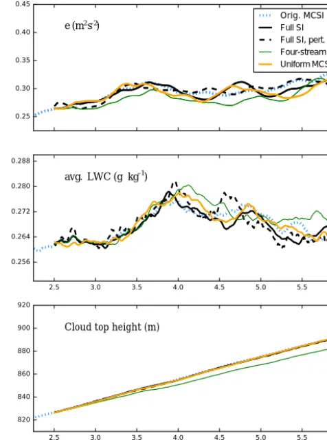
number of radiative transfer calculations is on the order of 100. As a result, it becomes unacceptable to perform a full spectral integration at every dynamical time step, even with simple 1-D two-stream solvers. This means that in most mod-els, radiative transfer is performed at a lower rate than other physical processes. Pincus and Stevens (2009) proposed that instead of calculating radiative transfer spectrally dense and temporally sparse, one may sample only one spectral band at every model time step. The argument is that the error which is introduced by the coarse spectral sampling is averaged out over time and remains random and uncorrelated in space and time. As we mentioned in Sect. 2.1, the 3-D radiative trans-fer necessitates to compute the entire domain for one and the same spectral band instead of individual bands for each ver-tical column. In the following we will refer to the adapted version as the uniform Monte Carlo spectral integration. The uniform sampling relaxes the assumption that the errors are uncorrelated in space and it is therefore not clear whether it is still valid. We repeated the numerical experiment in close re-semblance to the original paper of Pincus and Stevens (2009) and examine the results to validate the applicability of the uniform Monte Carlo spectral integration.
There, they used the model setup for the DYCOMS-II sim-ulation (details in Stevens et al., 2005). They show results for nocturnal simulations. In contrast, here we show results with a constant zenith angle θ=45◦. Radiative transfer is com-puted with a 1-D delta-Eddington two-stream solver. The simulation is started with Monte Carlo spectral integration and from 2.5 h on, also calculated with the full spectral in-tegration and the uniform Monte Carlo spectral inin-tegration. Note the good agreement between the full spectral sampling simulation and the one with the original Monte Carlo spec-tral integration in Fig. 1. The uniform formulation of Monte Carlo spectral integration leads to high-frequency changes in the average liquid water content (LWC). These fluctuations in LWC do however not lead to major differences in the evo-lution of the boundary layer clouds or turbulent kinetic en-ergy. To put the changes in LWC into perspective, we ran the simulation again with a random perturbation on the boundary layer temperature field. The perturbation is randomly drawn from the interval between−0.5 and 0.5 K. We find that the temperature perturbation induces similar differences to the flow as does the Monte Carlo spectral integration. Further-more, we additional ran the simulation with theδfour-stream solver (Liou et al., 1988). While arguably both are good ra-diative transfer solvers, the choice of the solver leads to big-ger differences than the uniform Monte Carlo spectral in-tegration and even introduces a bias in the evolution of the cloud height. We therefore conclude, that while the uniform Monte Carlo spectral integration may very well introduce considerable small-scale errors, it nevertheless seems to be a viable approximation for this kind of simulation. Addi-tionally, we repeated the same kind of experiment for sev-eral other scenarios (broken cumulus and deep convection),
0.25 0.30 0.35 0.40 0.45
e (m s )2 –2 Orig. MCSI
Full SI Full SI, pert. Four-stream Uniform MCSI
2.5 3.0 3.5 4.0 4.5 5.0 5.5 6.0
0.256 0.264 0.272 0.280 0.288
avg. LWC (g kg )
2.5 3.0 3.5 4.0 4.5 5.0 5.5 6.0
Forecast time (h)
820 840 860 880 900 920
Cloud top height (m) –1
Figure 1. Intercomparison of the DYCOMS-II simulation, once
forced with the full radiation (solid line), with the original Monte Carlo spectral integration (dotted) and with the uniform ver-sion (dashed). The dash-dotted line is a calculation with full spectral integration but with the four-stream solver instead of the two-stream solver. The top panel displays the vertically integrated turbulent ki-netic energy, the middle panel displays the mean liquid water con-tent (conditionally sampled and weighted by physical height), and the bottom panel displays the mean cloud top height.
all confirming the applicability of the uniform Monte Carlo spectral integration.
4 Performance statistics
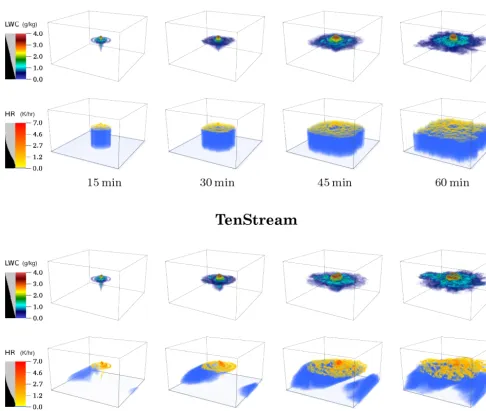
Figure 2. Volume-rendered perspective on liquid water content and solar atmospheric heating rates of the warm-bubble experiment
(initial-ized without horizontal wind). The two upper panels depict a simulation which was driven by 1-D radiative transfer and the two lower panels show a simulation where radiative transfer is computed with the TenStream solver (solar zenith angleθ=60◦; constant surface fluxes). Three-dimensional effects in atmospheric heating rates introduce anisotropy which in turn has feedback on cloud evolution. Domain dimen-sions are 12.8×12.8 km horizontally and 5 km vertically at a resolution of 50 m in each direction. See Sect. 6 for simulation parameters. Gray bar in the legend determines the transparency of the individual colors for the volume renderer.
4.1 Strong scaling
We hypothesized earlier (Sect. 2.2) that a good initial guess for the iterative solver results in a faster convergence rate. To test this assumption we performed two strong-scaling (prob-lem size stays the same) simulations. One clear-sky experi-ment without clouds in which the difference between radia-tion calls is minimal and a warm-bubble case with a strong cloud deformation and displacement between time steps.
These two situations enclose what the solver may be used for and are hence the extreme cases with respect to the com-putational effort.
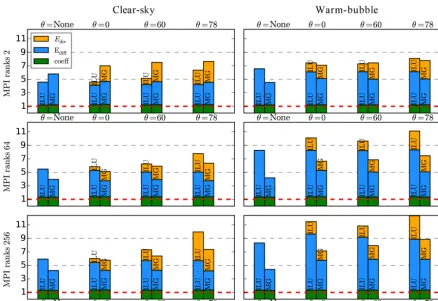
Figure 3. Two strong-scaling tests for a clear sky and a strongly forced scenario. Vertical axis is the increase of computational time normalized
to a delta-Eddington two-stream calculation (solvers only). Horizontal axis is for different solar zenith angles (θ =None means thermal only, no solar radiation). The stacked bars denoting time used for the individual components of the solver. “Coeff” is the time needed to retrieve and interpolate the transport coefficients.Ediffis the elapsed time that was used to set up the source term and solve for the diffuse radiation;
the same for the direct radiation inEdir. The bars are labeled with the corresponding matrix preconditioning.
cloud microphysics, a constant surface temperature without Monte Carlo spectral integration, and a dynamic time step of about 2 s.
Both scenarios are run forward in time for an hour for dif-ferent solar zenith angles and with varying matrix solvers and preconditioners (presented in Sect. 2.2.1). The difference be-tween the first and the second simulation is the external forc-ing that was applied. The clear-sky case is initialized with less moisture, weaker initial wind, and no temperature pertur-bation. No clouds develop in the course of the simulation. In contrast, the second case is initialized with a saturated mois-ture profile, a strong wind field and a positive, bell-shaped temperature perturbation in the lower atmosphere. The tem-perature perturbation leads to a rising warm bubble which leads to a cloud shortly after. The initial forcing and latent heat release leads to strong updrafts up to 19 m s−1 while the horizontal wind with up to 15 m s−1 quickly displaces the cloud sidewards. This strong deformation should give an upper bound on the dissimilarity between calls to the radi-ation scheme and therefore reduce the quality of the initial guess. To illustrate the general behavior of the strong and weak-scaling experiments, Fig. 2 depicts the warm bubble
simulation (for the purpose of visualization without initial horizontal wind) – once driven by 1-D radiative transfer and once more with the TenStream solver.
Table 1. Details on the computers used in this work. Mistral and
Blizzard are Intel–Haswell and IBM Power6 supercomputers at DKRZ, Hamburg, respectively. Thunder denotes a Linux Cluster at ZMAW, Hamburg. Columns are the number of MPI ranks used per compute node, the number of sockets and cores, and the maxi-mum memory bandwidth per node as measured by the streams (Mc-Calpin, 1995) benchmark.
Ranks/ Cores Memory
node bandwidth
Mistral 24 2×[email protected] GHz 112 GB s−1 Blizzard 64 4×[email protected] GHz 37 GB s−1
Thunder 16 2×[email protected] GHz 76 GB s−1
conditions. The clear-sky simulations are computationally cheaper than the more challenging cloud producing warm-bubble simulations. In the former, the solver often converges in just one iteration whereas in the latter rather complex case, more iterations are needed. Note that the ILU precondition-ing weakens if more processors are used. The ILU is a serial preconditioner and in the case of parallel computations, it is applied to each subdomain independently. The ILU precon-ditioner hence can not propagate information between pro-cessors.
The performance of GAMG is less affected by paralleliza-tion. The number of iterations until convergence stays close to constant (independent of the number of processors). The GAMG preconditioning outperforms the ILU precondition-ing for multicore systems whereas the setup cost of the coarse grids as well as the interpolation and restriction operators are more expensive if the problem is solved on a few cores only. In summary, we expect the increase in runtime compared to traditionally employed 1-D two-stream solvers to be in the range of 5–10 times.
4.2 Weak scaling
We examine the weak-scaling behavior using the earlier pre-sented simulation (see Sect. 4.1) but run it only for 10 min. The experiment uses multigrid preconditioning and only per-forms calculations in the thermal spectral range. The number of grid points is chosen to be 16 by 16 per MPI rank (≈105 unknown fluxes or ≈106 transfer coefficients per proces-sor). The simulations were performed at three different ma-chines/networks (see Table 1). Please note that the simu-lations for Mistral (see Table 1) do not fill up the entire nodes (24 cores) since UCLA-LES can currently only run on a number of cores which is a power of two.
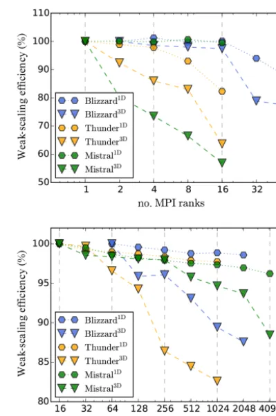
Figure 4 presents the weak-scaling efficiencyf, defined by f =tsingle core
tmulti core ·100 %. The scaling behavior can be sepa-rated into two regimes: the efficiency on one compute node and the efficiency of the network communication. As long as we continue to use one node (Fig. 4), the loss of scal-ing concerns the 3-D TenStream solver as well as the 1-D
Figure 4. Weak-scaling efficiency running UCLA-LES with
inter-active radiation schemes. Experiments measure the time for the ra-diation solvers only (i.e., no dynamics or computation of optical properties). Timings are given as a best of 10 runs. Weak-scaling efficiency is given for the TenStream solver (triangle markers) as well as for a two-stream solver (hexagonal markers). Scaling behav-ior compared to single core computations (remaining on one com-pute node)(left). Comcom-pute node parallel scaling (normalized against a single node)(right). The individually colored lines correspond to different machines (see Table 1 for details) and calculations once done with the delta-Eddington two-stream solver (hexagons) and once with the TenStream solver (triangles).
two-stream solver. Reasons for the reduced efficiency may be cache issues, hyperthreading, or memory-bus saturation. The scaling behavior for more than one node (Fig. 4) shows a close to linear scaling for the 1-D two-stream solver and a decrease in performance in the case of the TenStream solver. The limiting factor here is network latency and throughput.
5 Conclusions
We described the necessary steps to couple the 3-D Ten-Stream radiation solver to the UCLA-LES model. From a technical perspective, this involved the reorganization of the loop structure, i.e., first calculate the optical properties for the entire domain and then solve the radiative transfer.
end, we conducted numerical experiments (DYCOMS-II) in close resemblance to the work of Pincus and Stevens (2009) and found that the Monte Carlo spectral integration holds true, even in case of horizontally coupled radiative transfer where the same spectral band is used for the entire domain.
The convergence rate of iterative solvers is highly depen-dent on the applied matrix preconditioner. In this work, we tested two different matrix preconditioners for the TenStream solver: first, an incomplete LU decomposition and second, the algebraic multigrid preconditioner, GAMG. We found that the GAMG preconditioning is superior to the ILU in most cases and especially so for highly parallel simulations.
The increase in runtime is dependent on the complexity of the simulation (how much the atmosphere changes be-tween radiation calls) and the solar zenith angle. We eval-uated the performance of the TenStream solver in a weak and strong-scaling experiment and presented runtime com-parisons to a 1-D delta-Eddington two-stream solver. The in-crease in runtime for the radiation calculations ranges from a factor of 5–10. The total runtime of the LES simulation in-creased roughly by a factor of 2–3. An only 2-fold increase in runtime allows extensive studies concerning the impact of 3-D radiative heating on cloud evolution and organization.
This study aimed at documenting the performance and ap-plicability of the TenStream solver in the context of high-resolution modeling. Subsequent work has to quantify the impact of 3-D radiative heating rates on the dynamics of the model.
6 Code availability
The UCLA-LES model is publicly available at https://github. com/uclales. The calculations were done with the modi-fied radiation interface which is available at git revision “bbcc4e08ed4cc0789b33e9f2165ac63a7d0573ef”.
Appendix A: Input parameters for the PETSc solvers
−k s p _ t y p e b c g s
−p c _ t y p e b j a c o b i
−s u b _ p c _ t y p e i l u
−s u b _ p c _ f a c t o r _ l e v e l s 1
Listing A1. Biconjugate gradient squared iterative solver. The block Jacobi preconditioner does an incomplete LU preconditioning on each
rank with fill level 1 independent of its neighboring ranks.
−k s p _ t y p e f g m r e s
−k s p _ r e u s e _ p r e c o n d i t i o n e r −p c _ t y p e gamg
−p c _ g a m g _ t y p e agg
−p c _ g a m g _ a g g _ n s m o o t h s 0 −p c _ g a m g _ t h r e s h o l d . 1 −p c _ g a m g _ s q u a r e _ g r a p h 1
−m g _ l e v e l s _ k s p _ t y p e r i c h a r d s o n −m g _ l e v e l s _ p c _ t y p e s o r
−m g _ l e v e l s _ k s p _ m a x _ i t 5
Listing A2. Flexible GMRES solver with algebraic multigrid preconditioning. This uses plain aggregation to generate coarse
Acknowledgements. This work was funded by the Federal Ministry of Education and Research (BMBF) through the High Definition Clouds and Precipitation for Climate Prediction (HD(CP)2) project (FKZ: 01LK1208A). Many thanks to Bjorn Stevens and the DKRZ, Hamburg for providing us with the computational resources to conduct our studies.
Edited by: K. Gierens
References
Balay, S., Abhyankar, S., Adams, M. F., Brown, J., Brune, P., Buschelman, K., Eijkhout, V., Gropp, W. D., Kaushik, D., Kne-pley, M. G., McInnes, L. C., Rupp, K., Smith, B. F., and Zhang, H.: PETSc Users Manual, Tech. Rep. ANL-95/11 – Revision 3.5, Argonne National Laboratory, 2014.
Di Giuseppe, F. and Tompkins, A.: Three-dimensional radiative transfer in tropical deep convective clouds, J. Geophys. Res.-Atmos., 108, 4741, doi:10.1029/2003JD003392, 2003.
Evans, K. F.: The spherical harmonics discrete ordinate method for three-dimensional atmospheric radiative transfer, J. Atmos. Sci., 55, 429–446, doi:10.1175/1520-0469(1998)055<0429:TSHDOM>2.0.CO;2, 1998.
Frame, J. W., Petters, J. L., Markowski, P. M., and Harrington, J. Y.: An application of the tilted independent pixel approxima-tion to cumulonimbus environments, Atmos. Res., 91, 127–136, doi:10.1016/j.atmosres.2008.05.005, 2009.
Fu, Q. and Liou, K.: On the correlated k-distribution method for radiative transfer in nonhomogeneous atmo-spheres, J. Atmos. Sci., 49, 2139–2156, doi:10.1175/1520-0469(1992)049<2139:OTCDMF>2.0.CO;2, 1992.
Harrington, J. Y., Feingold, G., and Cotton, W. R.: Radiative impacts on the growth of a population of drops within simu-lated summertime arctic stratus, J. Atmos. Sci., 57, 766–785, doi:10.1175/1520-0469(2000)057<0766:RIOTGO>2.0.CO;2, 2000.
Hogan, R. J. and Shonk, J. K.: Incorporating the effects of 3D radia-tive transfer in the presence of clouds into two-stream multilayer radiation schemes, J. Atmos. Sci., 70, 708–724, 2013.
Jakub, F. and Mayer, B.: A three-dimensional parallel radiative transfer model for atmospheric heating rates for use in cloud re-solving models – The TenStream solver, J. Quant. Spectrosc. Ra., 163, 63–71, doi:10.1016/j.jqsrt.2015.05.003, 2015.
Joseph, J., Wiscombe, W., and Weinman, J.: The Delta-Eddington approximation for radiative flux transfer, J. Atmos. Sci., 33, 2452–2459, doi:10.1175/1520-0469(1976)033<2452:TDEAFR>2.0.CO;2, 1976.
Klinger, C. and Mayer, B.: The Neighbouring Column Approxima-tion (NCA)-A fast approach for the calculaApproxima-tion of 3D thermal heating rates in cloud resolving models, J. Quant. Spectrosc. Ra., 168, 17–28, doi:10.1016/j.jqsrt.2015.08.020, 2015.
Liou, K.-N., Fu, Q., and Ackerman, T. P.: A simple formulation of the delta-four-stream approximation for radiative transfer param-eterizations, J. Atmos. Sci., 45, 1940–1948, 1988.
Marquis, J. and Harrington, J. Y.: Radiative influences on drop and cloud condensation nuclei equilibrium in stratocumulus, J. Geo-phys. Res.-Atmos., 110, D10205, doi:10.1029/2004JD005401, 2005.
Mayer, B.: Radiative transfer in the cloudy atmosphere, in: EPJ Web of Conferences, 1, 75–99, EDP Sciences, doi:10.1140/epjconf/e2009-00912-1, 2009.
McCalpin, J. D.: Memory Bandwidth and Machine Balance in Current High Performance Computers, IEEE Computer Soci-ety Technical Committee on Computer Architecture (TCCA) Newsletter, 19–25, 1995.
Mlawer, E. J., Taubman, S. J., Brown, P. D., Iacono, M. J., and Clough, S. A.: Radiative transfer for inhomogeneous atmospheres: RRTM, a validated correlated-k model for the longwave, J. Geophys. Res.-Atmos., 102, 16663–16682, doi:10.1029/97JD00237, 1997.
Muller, C. and Bony, S.: What favors convective aggre-gation and why?, Geophys. Res. Lett., 42, 5626–5634, doi:10.1002/2015GL064260, 2015.
O’Hirok, W. and Gautier, C.: The impact of model resolu-tion on differences between independent column approxima-tion and Monte Carlo estimates of shortwave surface irradiance and atmospheric heating rate., J. Atmos. Sci., 62, 2939–2951, doi:10.1175/JAS3519.1, 2005.
Petters, J. L.: The impact of radiative heating and cooling on ma-rine stratocumulus dynamics, available at: https://etda.libraries. psu.edu/paper/10199/5841, 2009.
Pincus, R. and Stevens, B.: Monte Carlo spectral integration: A con-sistent approximation for radiative transfer in large eddy sim-ulations, Journal of Advances in Modeling Earth Systems, 1, doi:10.3894/JAMES.2009.1.1, 2009.
Saad, Y.: A flexible inner-outer preconditioned GMRES algorithm, SIAM Journal on Scientific Computing, 14, 461–469, 1993. Saad, Y.: Iterative methods for sparse linear systems, Siam,
ISBN-10: 0898715342, 2003.
Schumann, U., Dörnbrack, A., and Mayer, B.: Cloud-shadow effects on the structure of the convective boundary layer, Meteorologis-che Zeitschrift, 11, 285–294, 2002.
Stevens, B., Moeng, C.-H., Ackerman, A. S., Bretherton, C. S., Chlond, A., de Roode, S., Edwards, J., Golaz, J.-C., Jiang, H., Khairoutdinov, M., et al.: Evaluation of large-eddy simula-tions via observasimula-tions of nocturnal marine stratocumulus, Mon. Weather Rev., 133, 1443–1462, doi:10.1175/MWR2930.1, 2005. Tompkins, A. M. and Di Giuseppe, F.: Generalizing cloud overlap treatment to include solar zenith angle effects on cloud geometry, J. Atmos. Sci., 64, 2116–2125, 2007.
Van der Vorst, H. A.: Bi-CGSTAB: A fast and smoothly converging variant of Bi-CG for the solution of nonsymmetric linear sys-tems, SIAM Journal on scientific and Statistical Computing, 13, 631–644, doi:10.1137/0913035, 1992.