M E T H O D O L O G Y
Open Access
Exploring the influence of short-term
temperature patterns on
temperature-related mortality: a case-study of
Melbourne, Australia
John L. Pearce
1*, Madison Hyer
1, Rob J. Hyndman
3, Margaret Loughnan
2, Martine Dennekamp
4and Neville Nicholls
2Abstract
Background:Several studies have identified the association between ambient temperature and mortality; however,
several features of temperature behavior and their impacts on health remain unresolved.
We obtain daily counts of nonaccidental all-cause mortality data in the elderly (65 + years) and corresponding meteorological data for Melbourne, Australia during 1999 to 2006. We then characterize the temporal behavior of ambient temperature development by quantifying the rates of temperature change during periods designated by pre-specified windows ranging from 1 to 30 days. Finally, we evaluate if the association between same day temperature and mortality in the framework of a Poisson regression and include our temperature trajectory variables in order to assess if associations were modified by the nature of how the given daily temperature had evolved.
Results:We found a positive significant association between short-term mortality risk and daily average temperature as mortality risk increased 6 % on days when temperatures were above the 90th percentile as compared to days in the referent 25–75th. In addition, we found that mortality risk associated with daily
temperature varied by the nature of the temperature trajectory over the preceding twelve days and that peaks in mortality occurred during periods of high temperatures and stable trajectories and during periods of increasing higher temperatures and increasing trajectories.
Conclusion:Our method presents a promising tool for improving understanding of complex temperature health
associations. These findings suggest that the nature of sub-monthly temperature variability plays a role in the acute impacts of temperature on mortality; however, further studies are suggested.
Keywords:Climate, Health, Heat events, Heat wave, Temperature-mortality, Weather
Background
It is well known that thermal stress is a major contributor in weather-related health burdens as epidemiologic studies of temperature exposure have well-illustrated that temperature influences population-level health in a nonlinear way, with extremes (hot or cold) tending to have the largest effects [1, 2]. This exposure-response
relationship is complex as‘hot’and‘cold’effects reveal a‘U’ or‘J’shaped dose–response with variable temporal patterns of association, as excessive heat typically demonstrates a rapid effect on mortality (less than 2 days) and the effects of excessive cold tend to be evident over a longer period (sometimes greater than two weeks) [1]. These effects have also been shown to persist or amplify over periods of successive days, a pattern often described as a heat or cold wave [3, 4]. Although findings have been consistent, the complex nature of this environmental health problem has led to many aspects remaining unresolved [5, 6].
* Correspondence:[email protected]
1Department of Public Health Sciences, Medical University of South Carolina,
135 Cannon Street, Charleston, SC 29403, USA
Full list of author information is available at the end of the article
One area of particular interest as of late has been temperature variability, as a changing climate is expected to not only increase average temperatures and the frequency of extreme temperature events but also the variability of temperature within seasons [7]. Recent research suggests that such concerns are warranted as temperature variability (i.e., swings in temperature) has been shown to be an important determinant of health [8–10]. For example, findings from an examination of within-day temperature variability (difference in daily min/max, a.k.a. diurnal temperature range) and day-to-day mean temperature differences in Brisbane, Australia suggest that temperature variability is associated with an increase in childhood pneumonia cases [9]. In east Asia, and examination of diurnal temperature range and mor-tality found greater effects on respiratory mormor-tality and the elderly [11]. In the US, recent findings from an investigation focused on whether the standard deviation of summer temperatures was associated with survival in four cohorts of persons over age 65 years with predisposing diseases found that long-term increases in temperature variability may increase risk of mortality in certain popula-tions [10]. Biologically speaking, such findings are plausible as it is well known that certain populations (e.g., elderly) have a more difficulty with thermoregulation and acclimatization, processes that may be challenged during periods of significant temperature shifts [12].
Collectively, these findings provide evidence that supports a hypothesis that changes in temperature can be harmful to health; however, more studies are needed to better understand how short-term variabil-ity in temperature behavior influences health. For ex-ample, it is still largely unclear whether or not rapid increases or decreases in temperatures influence health or if they act in combination with extremes to amplify effects. Such knowledge gaps are difficult to address and warrant the development of new methodologies.
In this study, our overarching objective is to illustrate a method that allows health investigators to explore the role of sub-monthly patterns of temperature change in the short-term relationship between temperature and human health. The driving hypothesis is that heterogen-eity in the nature of temperature change over sub-monthly periods (i.e., temperature trajectory) will impact the magnitude of short-term temperature associations with our health outcome. To address this hypothesis, we apply our method within the framework of an acute health effects study of temperature and elderly mortality using Melbourne, Australia as our case study. The city of Melbourne, with a population of approximately 3.9 million, presents an appropriate study region because of its distinguishing temperature extremes, relatively large elderly population (13 % > 65 years in 2006), and estab-lished literature on heat-related mortality [4].
Methods
This study is conducted in two stages. First, we develop a metric that characterizes the temporal trajectory of ambient temperature behavior by constructing linear models that define the pattern of temperature change (i.e., slope) over pre-specified windows of time. Then, we apply our metric in the framework of a well-established epidemiological modeling approach in order to estimate associations between temperature progressions and their interactions with ambient temperature on mortality while controlling for long-term trends and season.
Data
The data used in this study are concurrent time-series of daily mortality counts and weather summaries from Melbourne, Australia over the years 1999 to 2006. Daily mortality data were provided by the Australian Bureau of Statistics (http://www.abs.gov.au/) and are the aggre-gate counts of non-accidental daily deaths of individuals aged 65 years and over (65+) across Greater Melbourne. Daily automatic weather station observations for air temperature (°C) and dew-point temperature (°C) were pro-vided by the Bureau of Meteorology (www.bom.gov.au) for site number 086282 (Melbourne International Airport).
Characterizing temperature trajectories
Conceptually, we define the ‘temperature trajectory’of a daily temperature as the rate of change of temperature over the days preceding (pre-specified window) the current observation. For example, if today’s temperature is 28 °C and our window of interest is the preceding three days, then the trajectory is defined as the slope of temporal changes in temperature observations over those days. So, a positive slope indicates there was an overall trend in temperatures rising over the window of interest, a negative slope implies a decreasing trend, and a zero slope indicates stability or neither a decreas-ing or increasdecreas-ing trend.
We model temperature trajectories using ordinary least-squares regression, applied to windows of lengthw. Specifically, we define a given day’s temperature trajec-tory as the linear trend of temperature over the preced-ingwdays. LetTbe the total length of the time series of temperatures. Then for each value of t between w+ 1 and T, we estimate a simple regression trend equation over thewobservations prior to timet:
yi¼αt;w−βt;wð Þ þt−i εi;t;
where yi is the observed average temperature on day i,
εi,t is a random error term, andi=t−w,…,t. Thus,βt,w
windows were restricted to a 30 day maximum in order to focus on sub-monthly behaviors. For each trajectory, we evaluate basic statistical properties and relationships with daily temperature.
Epidemiologic analyses
We modeled associations between temperature and daily mortality counts using the framework of a Poisson gen-eralized linear model (GLM) allowing for overdispersion [13]. The dependent variable was the daily number of deaths in the elderly and the primary exposure of inter-est was ambient temperature. To control for potential confounding, our model included a natural spline term accounting for long-term trend and seasonality (degrees of freedom (df = 7 per year), an indicator term for day-of-the-week, a term for influenza hospitalizations (indi-cator of flu season), and a natural spline term for dew-point temperature, a measure of atmospheric moisture (df = 4). Using this base model, we estimate main effects for ambi-ent temperature using same day average temperature and temperature trajectory using our previously described vari-able βt,w. Potential effect modification of temperature was explored using a product-term model that included terms for all variables and products contained within product.
The main effects of temperature and temperature tra-jectory were estimated by fitting a Poisson GLM model to the daily mortality counts with log mean given by (Model 1):
logð Þ ¼μt αþs1ð Þ þt DOWtþδFLUtþs2ðDPTtÞ
þs3ð Þ þyt s4 βt;w
;
where tis the day in the study period, DOWt is a day-of-week factor, FLUtis the number of influenza-related hospital admissions, DPTt is the daily mean dew-point temperature, and s1,…,s4 are all smooth functions
estimated using natural splines.
Model 2 is identical to model 1 except that percentile-based categories were used instead of natural spline terms for temperatures and temperature trajectories. This can be expressed as:
logð Þ ¼μt αþs1ð Þ þt DOWtþδFLUtþs2ðDPTtÞ
þCtþDt;
where Ct is a percentile-based category factor for temperature yt and Dt is a percentile-based category factor for trajectoryβt,w.
The effect modification of temperature with mortality was estimated with Model 3 by adding the product term
s5(yt×βt,w) to Model 1, where s5 is a smooth function estimated using natural splines. Models were fitted in the R statistical environment version 3.2.1 [14] using the glm() modeling function.
Sensitivity analysis
As determination of the trajectory window length is an important decision, we compare the significance of our findings as a function of trajectory window by running our models 1 & 3 using output from trajectories with 1 day to 30-day window lengths.
Results
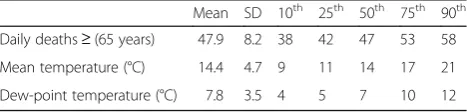
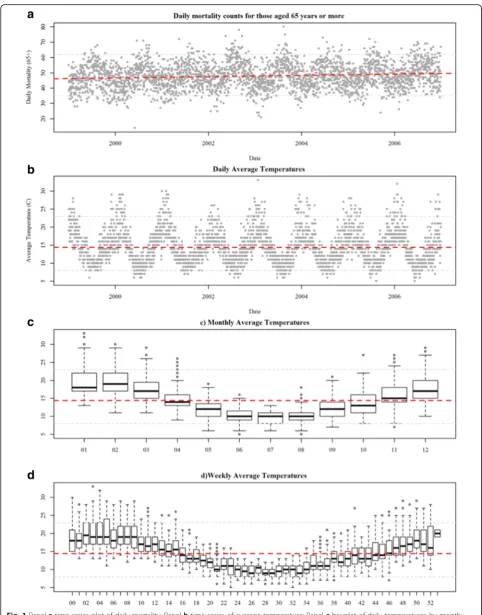
The average number of all-cause-non-accidental daily deaths in the elderly population for Melbourne during the study period was 48 persons per day with a mini-mum of 14 and a maximini-mum of 80 (Table 1). Mortality counts were higher in the cooler months but short-term fluctuations were obvious for all seasons (Fig. 1). A slight positive long-term trend was also visually apparent in the data and is consistent with trends in population growth [15].
During our study period, the mean daily average of temperature was 14 °C and the observed minimum daily average and maximum daily average temperatures were 5 and 33 °C, respectively. A strong oscillatory pattern was evident with peaks typically occurring during the warmer months of December through March (Fig. 1). In order to better understand shorter-term temperature behavior, we summarized daily average temperatures by month and week of the year during our study period. Monthly summaries reveal the greatest variability in daily temperature occurs during the warmer months (01–03; 1–12). Weekly summaries illustrate a similar pattern as variation was greater for weeks that occurred in the warmer months.
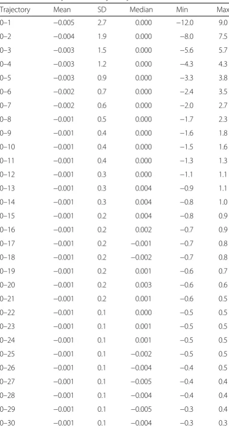
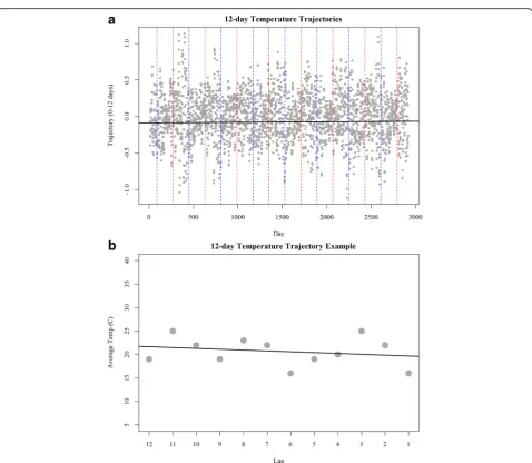
Trajectories were calculated for lengths of 1 to 30 days for average daily temperatures (Table 2). All trajectory windows were roughly normally distributed around 0 with variance reducing at similar rates as the trajectory window increases (Table 2). To illustrate, we chose to exemplify our method using a 12-day trajec-tory (Fig. 2). Evaluation of 12-day temperature tra-jectories illustrates no changes over the long-term; however, strong seasonal variations were evident, with larger magnitude trajectories being seen in the warmer months (Fig. 2a). This indicates that temperatures are more variable in warmer months. Using a 12-day period from our study, we illustrate how a trajectory captures the behavior of temperature change during our window of interest (Fig. 2b).
Table 1Summary statistics for elderly mortality (aged≥65 years.) and meteorology in Melbourne, Australia 1999 to 2006
Mean SD 10th 25th 50th 75th 90th
Daily deaths≥(65 years) 47.9 8.2 38 42 47 53 58
Mean temperature (°C) 14.4 4.7 9 11 14 17 21
The association between daily average temperature and the previous day’s temperature trajectory was weak over short windows and weakened as the trajectory window became larger (Fig. 3). Such low to moderate correlation indicates that multicollinearity should not be a major issue when applying this metric in a model with daily average temperature. It is important to note that correlations between trajectories were dependent upon their window differences, with similar windows being more correlated than dissimilar windows.
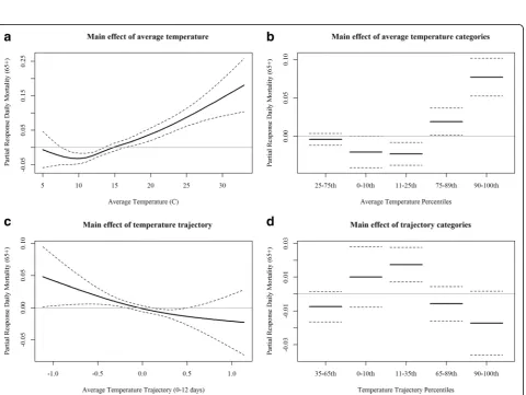
We investigated the main effects of same day average temperature and average temperature trajectory (0–12 days) using two models:model 1employs a natural spline term for our exposure metric of interest; andmodel 2 em-ploys an indicator term of percentile based categories. Both models identified temperature and temperature
trajectory as being significantly associated with elderly mortality. In model 1, we see the‘J’shaped response curve for temperature showing that higher temperatures posi-tively associate with elderly mortality in Melbourne (Fig. 4a). The effect of temperature maintained a similar response form in model 2, revealing an approximate 6 % increase in mortality on days when temperatures were above the 90thpercentile (≥21 °C) as compared to days in the referent 25-75thpercentile category (11–17 °C, Fig. 4b). For our temperature trajectory terms, models 1&2 suggest that periods of slightly decreasing temperatures over twelve days were most associated with daily mortality (Fig. 4 cd). In both models, the association for daily temperature was stronger than the association for temperature trajectory with mortality as indicated by residual deviance explained and p-values. For example, the residual deviance accounted for by temperature (p< 0.0001) in model 1 was 43.02 as compared to 10.08 for temperature trajectory (p= 0.0096).
Collectively, these results demonstrate that daily aver-age temperature and temperature trajectory associate with elderly mortality in Melbourne. Although not pre-sented here, it is important to note that evaluating daily maximum and minimum temperatures revealed similar findings as did the investigation of various lag terms (up to 14 days). The findings for average temperature were the strongest and thus were chosen to better facilitate testing for complex interactions. Sensitivity analysis of temperature trajectory window is presented in a later section.
Results from a product term model, model 3, identi-fied significant associations between average temperature (p< 0.0001), 12-day temperature trajectory (p= 0.01), and a product-term (p= 0.01). Visualization of the product-term effect demonstrates that the effect of daily average temperature varies between temperature trajec-tories (Fig. 5). We see that the effects peak when daily average temperatures are high during conditions when trajectories are near zero (i.e., periods of near stability). We also see mortality increases under higher tempera-tures with increasing trajectories. Daily mortality counts were found to be the lowest when temperatures were lowest and trajectories were at either extreme.
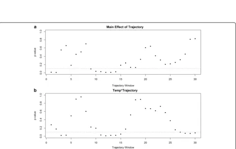
Plotting p-value estimates for variable trajectory windows using our main effects (model 1) and product-term model (model 3) reveal that specification of window length is an important decision (Fig. 6). Examination of p-values as a function of trajectory window length revealed that main effects for our trajectory window were significant for very short windows (0–2 days), moderate windows (9–14 days), and long windows (24–30 days). For product-terms, windows of 3 to 4 days, 11 to 15 days, and 28 to 30 days were significant (under 0.1).
Table 2Summary table of trajectory windows
Trajectory Mean SD Median Min Max
0–1 −0.005 2.7 0.000 −12.0 9.0
0–2 −0.004 1.9 0.000 −8.0 7.5
0–3 −0.003 1.5 0.000 −5.6 5.7
0–4 −0.003 1.2 0.000 −4.3 4.3
0–5 −0.003 0.9 0.000 −3.3 3.8
0–6 −0.002 0.7 0.000 −2.4 3.5
0–7 −0.002 0.6 0.000 −2.0 2.7
0–8 −0.001 0.5 0.000 −1.7 2.3
0–9 −0.001 0.4 0.000 −1.6 1.8
0–10 −0.001 0.4 0.000 −1.5 1.6
0–11 −0.001 0.4 0.000 −1.3 1.3
0–12 −0.001 0.3 0.000 −1.1 1.1
0–13 −0.001 0.3 0.004 −0.9 1.1
0–14 −0.001 0.3 0.004 −0.8 1.0
0–15 −0.001 0.2 0.004 −0.8 0.9
0–16 −0.001 0.2 0.002 −0.7 0.9
0–17 −0.001 0.2 −0.001 −0.7 0.8
0–18 −0.001 0.2 −0.002 −0.7 0.8
0–19 −0.001 0.2 0.001 −0.6 0.7
0–20 −0.001 0.2 0.003 −0.6 0.6
0–21 −0.001 0.2 0.001 −0.6 0.5
0–22 −0.001 0.1 0.000 −0.5 0.5
0–23 −0.001 0.1 0.001 −0.5 0.5
0–24 −0.001 0.1 0.001 −0.5 0.5
0–25 −0.001 0.1 −0.002 −0.5 0.5
0–26 −0.001 0.1 −0.004 −0.4 0.5
0–27 −0.001 0.1 −0.005 −0.4 0.4
0–28 −0.001 0.1 −0.004 −0.4 0.4
0–29 −0.001 0.1 −0.005 −0.3 0.4
Discussion
In this study, we sought to examine how the behavior of preceding days’ temperature impacted the relationship between daily temperature and elderly mortality. We achieved this by characterizing the rates of temperature changes on days preceding a daily temperature (i.e., temperature trajectory) and applied such characterization as an‘exposure’term in an epidemiologic model. As such, we were able to examine if the relationship between daily temperature and mortality varied by the preced-ing days trajectory.
Our study found a positive association between daily average temperature and elderly mortality (Fig. 5), with results demonstrating a ‘J’ shaped response as days characterized by higher temperatures were associated
Fig. 3Pearson correlation between daily average temperature and temperature trajectories
Fig. 5Product-term effects of average temperature and temperature trajectory (0–12 days) on mortality using a natural spline product-term in model 3
increased mortality. Another explanation is that this cooling trend could be identifying impacts during the colder months; however, we are using daily mortality data so our results are skewed towards warm season and high temperature relationships.
Of course, our primary interest here was exploring the influence temperature trajectory has as an effect modi-fier rather than a main effect; nevertheless, further re-search into this relationship is warranted. Results from our product-term model revealed that the effect of daily average temperature was modified by the nature of the preceding days’ temperature trajectory (Fig. 6). This is the key finding of the study as it illustrates how the behavior of temperature on days leading up to a daily temperature event influences the association with mor-tality. We found that the highest temperatures in com-bination with relative stability over the preceding 12 days (i.e., trajectory near zero) corresponded with the peaks in daily mortality. This finding suggests that a ‘heat wave’effect is occurring in Melbourne. This impact of temperature behavior agrees well with studies of heat/ cold events in the United States as well as other loca-tions around the globe [1, 16].
As our method is new, an important point of discus-sion is how it compares with previous approaches such as using more traditional lag terms and moving averages. The major distinction of our method is that it quantifies behavior change, in terms of directionality and magni-tude, rather than quantifying behavior. This has several advantages. Interpretatively, health investigators can now explore the magnitude and direction of temperature behavior, a feature that improves understanding of the role of temperature variability on public health. Statisti-cally speaking, when comparing trajectory of window (n) to lag-n term models, where n> 1, our approach is less sensitive to outlying days. Since the approach used to obtain trajectory values does not require the estimated line pass through the last value (lag-0) or require the first value (lag-n) to be the intercept, it estimates the overall temperature behavior. Furthermore, when com-paring a trajectory of window (n) to a (n+ 1)-day moving average, where n> 1, our approach is more robust in providing direction of change rather than simply quanti-fying behavior. Another benefit of our approach is that temperature trajectories were generally found to have little correlation with daily temperatures, a situation that provides the unique opportunity to approach modeling environmental effects on health outcomes with more detail without as much concern for issues of multicollinear-ity as may be found in lag term or moving average models.
Though our method is an innovative alternative to commonly used summary variables for temperature behavior, it does have limitations. One is that we per-formed a two-step approach and did not incorporate the
precision of the trajectory estimates into our analysis; thus we have introduced uncertainties that make it harder to interpret confidence intervals. Considerations were made for weighting by the inverse standard error or using a coefficient of variation but neither was used as these methods need to be refined to improve in-terpretation. For example, weighting trajectories by the inverse standard error would inevitably produce values where the temperature behavioral characteristics would no longer be distinguishable because all days of near equal inversely proportional values of trajectory and its standard error would be near equal regardless of the trajectory value. Moreover, both approaches would de-teriorate at trajectories close to zero as weighting by the inverse standard error would only produce another value close to zero, regardless of the standard error, and the coefficient of variation would approach infinity. Gener-ally speaking, the expected impact of this uncertainty is somewhat analogous to exposure misclassification and thus bias towards the null is the likely result. Further work should be done to include the precision of the tra-jectory estimate. Another limitation of this work is that our models treat the trajectory of temperature as linear, an assumption that may not always be true. As such, our analysis may have missed more subtle temperature be-havior impacts on health. In addition to methodological limitations, there are also additional limitations to the interpretability of our findings. For example, our study focuses on a single city and thus it is possible that our results may not be found in other locations. Thus, to improve the generalizability of our findings, future multi-city studies are recommended.
Possible future directions are rich with opportunities as there are several alternative approaches that could be used to capture patterns in changing temperatures over time. One such possibility could be considering a‘ float-ing-window’where the size of the trajectory window is a function of standardized expected temperature. Another alternative would be to include some function of tem-peratures in the models that would reduce concerns about uncertainty. However, such approaches need to be more fully developed as models are complex. Addition-ally, possibilities include modeling a mixture of trajec-tories in the context of single predictor models (i.e., temperature, single-pollutant, etc.) and multi-predictor models (i.e., multi-pollutant) models.
Conclusion
temperature and mortality. Overall, we found temperature trajectories are a very useful tool to investigate the associ-ation of temperature and mortality. Finally, our method-ology provides a new tool for public health scientists to better understand and prepare for the health impacts associated with a changing climate.
Abbreviations
DF:Degrees of freedom; GLM: Generalized linear model
Acknowledgements
Not Applicable.
Funding
This publication was made possible, in part, by funding provided by the Medical University of South Carolina and the National Institute of Environmental Health Sciences of the National Institutes of Health under Award Number K99/R00ES023475. The content is solely the responsibility of the authors and does not necessarily represent the official views of NIH.
Availability of data and materials
Environmental data used in this study were obtained from the Australian Bureau of Meteorology: http://www.bom.gov.au/. Data descriptions in the methods provide resources for access. Health outcome (mortality) data is available from the Australian Bureau of Statistics: http://www.abs.gov.au/ AUSSTATS/[email protected]/DetailsPage/3303.02014?OpenDocument. However, the data use agreements prohibit sharing of data in the format analyzed.
Authors’contributions
JP obtained the dataset, led the epidemiologic design of the study, performed analyses, and co-drafted the manuscript. MH introduced the idea of temperature trajectories, performed analyses, and assisted in drafting the manuscript. RH assisted with statistical modeling and revising the manu-script. NN, ML, and MD assisted with the conceptual application and revising the manuscript. All authors read and approved the final manuscript.
Competing interests
The authors declare that they have no competing interests.
Consent for publication
Not Applicable.
Ethics approval and consent to participate
Not Applicable.
Author details
1
Department of Public Health Sciences, Medical University of South Carolina, 135 Cannon Street, Charleston, SC 29403, USA.2School of Geography and
Environmental Science, Monash University, Wellington Rd., Clayton, Victoria 3800, Australia.3Department of Econometrics and Business Statistics, Monash
University, Wellington Rd., Clayton, Victoria 3800, Australia.4Department of Epidemiology and Preventative Medicine, Monash University, 99 Commercial Rd., Melbourne, Victoria 3004, Australia.
Received: 11 May 2016 Accepted: 29 October 2016
References
1. Anderson BG, Bell ML. Weather-Related Mortality: How Heat, Cold, and Heat Waves Affect Mortality in the United States. Epidemiol. 2009;20(2): 205–13.
2. Nordio F, Zanobetti A, Colicino E, Kloog I, Schwartz J. Changing patterns of the temperature–mortality association by time and location in the US, and implications for climate change. Enviro Intern. 2015;81:80–6.
3. Anderson G, Bell ML. Heat Waves in the United States: Mortality Risk during Heat Waves and Effect Modification by Heat Wave Characteristics in 43 U. S. Communities. Environ Health Perspect. 2010;119(2):210–8.
4. Nicholls N, Skinner C, Loughnan M, Tapper N. A simple heat alert system for Melbourne. Australia Intern J Biomet. 2008;52(5):375–84.
5. Hajat, S, Vardoulakis, S, Heaviside, C, and Eggen, B, Climate change effects on human health: projections of temperature-related mortality for the UK during the 2020s, 2050s and 2080s. J Epidemiol Comm Health. 2014;68(7); 641–8.
6. Mills D, Schwartz J, Lee M, Sarofim M, Jones R, Lawson M, Duckworth M, Deck L. Climate change impacts on extreme temperature mortality in select metropolitan areas in the United States. Clim Chng. 2015;131(1):83–95. 7. Change IC. The Physical Science Basis: Working Group I Contribution to the
Fifth Assessment Report of the Intergovernmental Panel on Climate Change. New York: Camb Uni Press; 2013. 1. p. 535–1.
8. Bobb JF, Peng RD, Bell ML, Dominici F. Heat-related mortality and adaptation to heat in the United States. Environ Health Perspect. 2014;122(8):811. 9. Xu Z, Hu W, Tong S. Temperature variability and childhood pneumonia: an
ecological study. Environ Health. 2014;13(1):1.
10. Zanobetti A, O’Neill MS, Gronlund CJ, Schwartz JD. Summer temperature variability and long-term survival among elderly people with chronic disease. Proceed Nat Acad Sci. 2012;109(17):6608–13.
11. Kim J, Shin J, Lim Y-H, Honda Y, Hashizume M, Guo YL, Kan H, Yi S, Kim H. Comprehensive approach to understand the association between diurnal temperature range and mortality in East Asia. Sci Tot Environ. 2016;539:313–21. 12. Kenny GP, Yardley J, Brown C, Sigal RJ, Jay O. Heat stress in older individuals
and patients with common chronic diseases. Can Med Assoc J. 2010; 182(10):1053–60.
13. Dominici F, McDermott A, Zeger SL, Samet JM. On the use of generalized additive models in time-series studies of air pollution and health. Am J Epidemiol. 2002;156(3):193–203.
14. Team RC. R: A language and environment for statistical computing. Vienna, Austria: R Foundation for Statistical Computing; 2013. p. 2014. ISBN 3-900051-07-0.
15. ABS. In: Government A, editor. Regional Population Growth, Australia 2008–2009. Canberra: Australian Bureau of Statistics; 2010.
16. Basu R. High ambient temperature and mortality: a review of epidemiologic studies from 2001 to 2008. Environ Health. 2009;8–40.
• We accept pre-submission inquiries
• Our selector tool helps you to find the most relevant journal
• We provide round the clock customer support
• Convenient online submission
• Thorough peer review
• Inclusion in PubMed and all major indexing services • Maximum visibility for your research
Submit your manuscript at www.biomedcentral.com/submit