The Stringency of Environmental Regulations and
Technological Change: A Specific Test of the Porter
Hypothesis
Maryam Asghari∗
Abstract
rade creates wealth through economic growth, and increased level of income effects environment in different ways. Firstly, when people become wealthier, their demand for environmental protection will increase because their priorities will change from employment, income, food or housing to more qualitative measures such as cleaner environment. Through increased level of income, trade can save people from the poverty versus environmental degradation circle which forces the poor people to exploit the environment in order to survive. Secondly, with rising level of national income, the governments and/or private firms could increase the expenditures targeting environmental development. These changes resulting from wealth increase may also improve environmental rules and regulations. Usually the goal of environmental policies is to protect the environment by imposing restrictions on firms and/or consumers. These policies are often criticised as it is claimed that the international competitiveness of domestic firms is reduced. However, in contrast to this cost biased argument Michael Porter formulated the hypothesis that environmental policies could also serve as a vehicle to enhance the competitiveness. However, Michael Porter formulated the hypothesis that says environmental policy spurs innovation which makes firms better off in the long run, since it increases their competitiveness (Porter (1991), Porter and van der Linde (1995)). The aim of this paper is test for the validity of the Porter hypothesis and trade liberalisation effect on environment in the EU, the Persian Gulf and in North-South countries regions. Our results confirm the Porter hypothesis in these regions. Also, trade liberalisation increases the CO2 emission per capita in the Persian Gulf, EU and North-South countries regions.
Keywords: Trade, Innovation, Environment, Growth, Porter hypothesis.
∗ Researcher in Environmental Economics and International Trade and Assistant Professor at Shahid Ashrafi Esfahani University, Esfahan,Iran
1- Introduction
The interaction between trade flows and environmental regulations has become quite a topical issue recently. There is a common belief that by applying more lenient environmental regulations, countries tend to reduce production costs of their manufactures and thus improve their ability to export, despite the possibility to become pollution havens. There have been many empirical studies performed in this field, trying to estimate this relationship. Empirical results provide non univocal results supporting this relationship (Antweiler et al., (2001); Bommer, (1999); Copeland and Taylor, (2003); Grether and De Melo, (2003); Letchumanan and Kodama, (2000), Levinson and Taylor, (2004), among the others). On the contrary, the theory of dynamic competitiveness deriving from technological innovation linked to stringent environmental standards has been exposed fashionably by Porter and van der Linde (1995).
The literature on the determinants of innovation is vast. Yet, most of this literature focuses on particular determinants of innovation, and only small parts of this literature focus on environmental innovation. Contemporary research on the relationship between environmental innovation and regulation is based on the assumption that technology push and market pull factors, firm internal conditions, and regulatory conditions drive the extent and form of environmental innovations.
Environmental regulation is viewed in neoclassical economics as a means to force firms to internalize external costs they would otherwise impose on society. Environmental regulation is (or rather should be), therefore, implemented in cases of market failure. Though, in principle, its necessity under conditions of market failure is uncontested in environmental economics (Rennings, (1998)), the policies to be chosen (instrument type) in particular cases and the stringency of regulation are very much subject to debate.
Traditionally, the neoclassical economic view has been that (strict) regulation has negative effects on productivity and competitiveness, as it leads to higher expenses by businesses and imposes constraints on industry behavior. Regulation can also increase uncertainty associated with future investments, so that they are postponed.
competitiveness. However, integrated approaches to innovation which design technologies with built-in environmental advantages can trigger competitive advantages.
The study suggests that environmental policy can stimulate innovation and trigger a positive contribution to competitiveness if the policy goes hand in hand with company environmental strategy and customer requirements. Companies stressed that a sufficient planning strategy is necessary to successfully comply with environmental legislation.
The “Porter hypothesis” has spurred substantial amounts of research on the influence of environmental regulation on innovation. While adherents of the Porter hypothesis have sought to demonstrate the empirical relevance of the win-win claim, neoclassical economists have argued that such win-win opportunities are exceptions. They have pointed to significant compliance costs of industry, competitive disadvantages of domestic firms in international markets, and opportunity costs of forced environmental activities (e.g., Jaffe et al., (1995); Palmer et al., (1995)). The Porter hypothesis says that environmental policy spurs innovation which makes firms better off in the long run, since it increases their competitiveness (Porter, (1991), Porter and van der Linde, (1995)).
The main argument is that firms are not aware of certain opportunities and that environmental policy might open the eyes. This results in a win-win situation in the sense that environmental policy improves both environment and competitiveness. The hypothesis is criticized by economists who argue that extra costs are not needed to trigger fruitful innovations and adopting modern machines that are more profitable. In rational economic modeling it cannot be explained why firms do not see these opportunities by themselves, which at least implies that the argument does not have a general validity.
in an increase of average productivity. The conclusion concerning the validity of the Porter hypothesis is that a win-win situation will not hold, but the decrease in competitiveness due to the extra environmental costs is mitigated by the modernization effect.
Porter identifies two different effects in which the objectives of environmental improvements and enhanced competitiveness can be combined in a win-win situation (Porter et al., (1995)): firstly, meeting a more stringent environmental regulation leads directly to competitive advantages for companies through the need for innovations (‘innovation effect’).
Innovation effect is that a strict environmental regulation triggers the discovery and introduction of cleaner technologies and environmental improvements, making production processes and products more efficient in terms of resource productivity. As well as affecting the economy as a whole, these competitive advantages also result in benefits for individual companies. Porter estimates that in many cases, the cost savings that can be achieved are sufficient to overcompensate for both the compliance costs directly attributed to new regulations and the innovation costs.
Secondly, companies achieve a technological advantage over the international competition leading to ‘first mover advantages’. Competitive advantages are linked to the rising environmental awareness observed throughout the world – but they can only emerge to the extent that national environmental standards anticipate and are consistent with international trends in environmental protection. Competitive advantages will arise for corporations under the regulation in this region as soon as international policy diffusion occurs. This ‘first mover advantage’ comprises using innovative technologies for the first time which, owing to learning curve effects or patenting, attain a dominating competitive position. At the macroeconomic level, a first mover position can also prove efficient if the competitive disadvantages of the polluting industry are compensated (or overcompensated) by first mover advantages of the environmental protection industry.
before, then its benefits will not be enough to fully offset the costs of compliance after stricter regulations are enforced.
The aim of this paper is test for the validity of the Porter hypothesis in the region of EU, Persian Gulf countries and in North-South region. In this paper we will try to shed some light on this possible virtuous cycle between increasing competitiveness, technology diffusion analyzing a very specific industrial sectors and environmental regulations, such as country’s net tax on dirty products, to test validity of the Porter hypothesis. The empirical model used in this context is based on the Heckscher-Ohlin model for international trade flows, following many other empirical studies focusing on the effects of environmental policy that spurs innovation on environmental quality.So, we need an overview of the relationships between trade, environment and growth for explanation of our model.
The rest of the paper is structured as follows: Section 2 gives an overview of the relationships between trade and environment; Section 3 examines the relationships between growth and environment; Section 4 describes the dataset, the methodology used and the main empirical results, and Section 5 summarizes the results and offers policy implications.
2- Trade and the Environment
Economic globalization may induce severe impacts on the environment and sustainable development. Globalization contributes to economic growth, accelerates structural changes, diffuses capital and technology and could magnify market failures and policy distortions. This could increase environmental damages. Globalization may act as a motor for improved prospects of international economic growth in some industries and sectors, but could also conceivably reduce economic prospects in other countries. This may result in poverty-induced resource depletion and environmental degradation.
To better understand how globalization-induced free trade impacts the environment, it is necessary to examine the channels through which such impacts are transmitted. There are tree such channels: (a) scale of economic activity; (b) composition effects; (c) technology effects (Antweiler et al., (2001)).
positive effects, when increased trade induces better environmental protection through economic growth and policy development that stimulates product composition and technology shifts that cause less pollution per unit of output.
- Composition effects: changes in the patterns of economic activity or micro-economic production, consumption, investment, or geographic effects from increased trade that either exerts positive environmental effects or cause negative consequences.
- Technology effects: either positive effects from reducing pollution per
unit of product, or negative effects from the spread of "dirty" technologies.
Copeland and Taylor (1995) allow for an arbitrary number of countries; they consider the cases of large and small number of countries to isolate the effects of terms of trade motivations for pollution policy from purely environmental motives. Pollution targets are implemented with a marketable permit system. Main results of this paper are: (i) if human capital levels differ substantially across countries, then a movement from autarky to free trade raises world pollution; if they are similar, world pollution does not rise with free trade (the driving force behind these is whether factor prices, including pollution permit prices, are equalized or not through trade); (ii) when free trade in goods raises world pollution, allowing for international trade in pollution permits can counteract this rise in global pollution (because pollution permit prices will get equalized and pollution-haven effect will be eliminated); (iii) untied international transfers of income lower the recipient's pollution but raise the donor's pollution, and thus may have no effect on global pollution as well as on prices and surprisingly on welfare levels of either country; on the other hand, income transfers tied directly to pollution reduction can be welfare enhancing. This last result underlines the potential importance of income effects both in analyzing global pollution reform and in determining how international trade affects the global environment.
The study by Antweiler, Copeland, and Taylor (1998) referred to suggests that total emissions could fall. The empirical evidence is based on the relationship between trade and ground level SO2 concentration. The data
polluting way for capital-abundant countries. This suggests that classical factors of comparative advantages are important, but also for the poorest countries, in which lax environmental regulations may have had an influence. In other words, SO2-intensive production seems to be migrating
from middle-income countries to both richer and poorer countries, leaving the net composition effect on the environment undetermined. At the same time, the technique effect seems to dominate the scale effect.
Cole and Elliott (2003)examine the impact of environmental regulation on trade patterns within the traditional comparative advantage based model and within the “new” trade theoretic framework. No influence is found in the first case, whereas the shares of trade that are inter-industry and intra-industry appear to be affected by environmental regulation differentials between two countries.
One of the most recent contributions is due to Frankel and Rose (2002). The authors note that the empirical analysis has to address a formidable simultaneity problem. They solve it by using appropriate instrumental variables in a two-equation system. Their econometric results for SO2, NO2,
and SPM suggest that growth has a beneficial effect on pollution and that a higher ratio of trade to income seems if anything to reduce air pollution. These results do not hold in the case of other broader measures of environmental quality. In particular, the optimistic story does not hold for CO2 emissions, where trade and growth alone are not sufficient, but
international cooperation is needed for this sort of global environmental problem.
3- Economic Growth and the Environment
The environmental Kuznets hypothesis (EKC) predicts an inverse U-shaped relationship between environmental pollution on the one hand and per capita income on the other. This shape is due to the scale, composition, income and technique effects. At first, the increasing scale of economic activity as well as its changing composition from agricultural towards industrial activities generates more pollution. However, as income rises, demand for environmental quality increases and governments introduce more stringent environmental regulation. This income effect, the replacement of old technologies by environmentally less harmful ones, together with the changing composition away from an industrial towards a post-industrial economy puts downward pressure on pollution. Eventually, as income passes some threshold level, better techniques, an increased demand for environmental quality and the composition effect outweigh the scale effect and environmental quality increases with growth.
However, the EKC, despite its theoretic micro-foundations, is ultimately an empirical relationship, which has been found to exist for some pollutants but not for others. There is nothing inevitable or optimal about the shape and height of the curve. First, the downturn of EKC with higher incomes may be delayed or advanced, weakened or strengthened by policy intervention. It is not the higher income per se which brings about the environmental improvement but the supply response and policy responsiveness to the growing demand for environmental quality, through the enactment of environmental legislation and development of new institutions to protect the environment.
Second, since it may take decades for a low-income country to cross from the upward to the downward sloping part of the curve, the accumulated damage in the meantime may far exceed the present value of higher future growth, and a cleaner environment, especially given the higher discount rates of capital constraint on low-income countries.
Therefore, active environmental policy to mitigate emissions and resource depletion in the earlier stages of development may be justified on purely economic grounds. In the same vein, current prevention may be more cost effective than a future cure, even in present value terms.
While this depends in part on income level (stage of development), the efficiency of markets and policies largely determines the height of the EKC curve. Where markets are riddled with failures (externalities, ill-defined property rights, etc.), or distorted by subsidies of environmentally destructive inputs, outputs and processes, the environmental price of economic growth is likely to be significantly higher than otherwise. Economic inefficiency and unnecessary environmental degradation are two consequences of market and policy failures that are embodied to different degrees in empirically estimated EKCs.
Higher incomes induce higher consumption that could increase environmental externalities but also raise the willingness to pay for environmental improvement. On the other hand, economic growth increases potential resources for environmental protection that raises environmental quality.World economic trade liberalization may help decrease pressures on developing countries to encroach on natural resources. But free trade and increased competition could also lead to decreased access to international technology standards or capital uses in developing regions. Trade liberalization may reinforce the vicious circle between poverty and environmental degradations. Free trade and international competition could force environmental depletion as it is exploited for exports. Studies on income levels and environmental degradation found an inverted U-shaped relationship (Grossman et al. (1995)). At low income levels, income growth is associated with higher levels of environmental degradation until a turning point is reached. Beyond this average income level, further income increases environmental improvement results. Environmental degradation could therefore be reduced by increased economic income rather than through targeted environmental policies.
The first empirical EKC study was the NBER working paper by Grossman and Krueger (1991) that estimated EKCs for SO2 , dark matter
enough to offset the greater level of economic activity, leading eventually to an improvement in environmental quality. Some have interpreted this to imply that countries might be able to outgrow environmental problems. (Holtz-Eakin et autres (1995))
The GEMS dataset is a panel of ambient measurements from a number of locations in cities around the world. Each regression involved a cubic function in levels (not logarithms) of PPP per capita GDP and various site-related variables, a time trend, and a trade intensity variable. The turning points for SO2 and dark matter were at around $4,000-5,000 while the
concentration of sus-pended particles appeared to decline even at low income levels. At income levels over $10,000-15,000, Grossman and Krueger’s estimates show increasing levels of all three pollutants.
Two sets of factors contribute to an early and rapid increase in abatement: i) on the technology side, large direct effects of growth on pollution and a high marginal effectiveness of abatement, and ii) on the demand side (preferences), rapidly declining marginal utility of consumption and rapidly rising marginal concern over mounting pollution levels. To the extent that development reduces the carrying capacity of the environment, the abatement effort must increase at an increasing rate to offset the effects of growth on pollution.
4- Estimation Method and Results
4-1- Our Model
In this research we will use ACT (Antweiler-Copeland-Taylor) model and Panel Data method. ACT model based on the Hercksher-Ohlin (HO) and the Stolper-Samuelson theorems because of trade theory based on the Hercksher-Ohlin (HO) theorem predicts that trade liberalisation leads to greater specialisation and a rise in national income in participating countries, following a more rational global allocation of production inspired by the principle of comparative advantage. In labour-abundant countries, trade liberalisation is expected to switch production from capital-intensive and inefficient import-substitutes towards efficient labour-intensive exportables. In turn, the Stolper-Samuelson theorem posits that such shift leads to the convergence in the prices of goods and factor remunerations. Because of this, domestic inequality is expected to decline in countries endowed with an abundant labour supply and to rise in those with an abundant endowment of capital, as the demand and remuneration of the latter (that exhibits an unequal income distribution) will increase, while the demand and remuneration of labour (that is distributed more equitably) will fall. The evidence on the impact of trade liberalisation on environment is, however, mixed.
To test the main assertions of the theory, our empirical analysis proceeds by examining environmental stringency levels between countries. The finding a dynamic measure of environmental stringency to test our hypotheses is a difficult task. We restricted our search over environmental measures that have both within-country and between-country variation so we could control for important unobservable factors that may influence the level of stringency. We chose a measure based on the tax on goods. Our proxy for the level of environmental stringency is the policy of net tax on dirty products.
I include the interaction between trade intensity and the net tax on dirty products to capture the environmental policy when trade is liberalized in the three regions. Based on our theoretical considerations, I estimate the following equation using fixed and random effects of panel data specifications.
Where
Eit includes the CO2 emission per capita.
GDPCit: GDP per capita is the scale effect. ACT separate scale effect by measuring the former using GDP/km2. Since we estimate national pollution emissions, the use of GDP/km2 is no longer meaningful as a measure of scale. We use GDP per capita as proxy for scale effect. It measures the increase in pollution that would be generated if the economy were simply scaled up, holding constant the mix of goods produced and production techniques. Trade and growth both increase real income, and therefore both increase the economy’s scale.
It-1, I2t-1: One lagged Gross national income per capita is the technique effect. Because we believe the transmission of income gains into policy is slow and reflects one period lagged, we use one period lagged Gross national income as our proxy for our technique effect. We have also allowed the technique effect to have a diminishing impact at the margin by entering both the level and the square of lagged Gross national income in all of our regressions.
Because trade liberalization raises income and environmental quality is a normal good, so trade liberalization could lead the government to tighten environmental policy which will lead to improve technique.
This use of lagged gross national income and its squared to capture technique effects is consistent with the environmental Kuznets curve literature. This literature is the inverted-U-shaped relationship between per capita income and pollution: increased incomes are associated with an increase in pollution in poor countries, but a decline in pollution in rich countries.
capital will increase the output of the capital-intensive industry, and reduce the output of the labor-intensive industry. An increase in the supply of labor stimulates of the labor-intensive industry and contracts of the capital-intensive industry.
The composition effect is critical in determining the effects of trade liberalization. Moreover, the sign of the composition effect is ultimately determined by a country’s comparative advantage. If a country has a comparative advantage in clean industries, then clean industries expand with trade; and conversely, if it has a comparative advantage in polluting industries, then dirty industries expand with trade. Therefore income increase in country and the people become wealthier then their demand for environmental protection will increase and the government imposes the more stringent environmental regulation.
OPit: We include trade intensity (the ratio of imports+exports to GDP) as a measure of trade frictions.
OPTaxit : Trade intensity is interacted with a country’s net tax on dirty products to capture the Porter hypothesis. Since more stringent environmental regulation spurs innovation in environmental protection as trade liberalized. In effect, more stringent environmental policy stimulates innovation since trade increases which in turn results in reduced exports and production of the dirty goods.1In Porter research environmental policy is treated as exogenous. A restrictive environmental policy lowers aggregate output because it imposes an additional constraint on the production possibilities set. In fact, in order to decrease pollution firms undertake abatement activities which result in increased production costs.
4-2- Data Sources
The time period covered in the estimations are 1980-2006 across the 6 countries of Persian Gulf (Iran, Kuwait, Oman, Bahrin, Saudi Arabic, United Arab Emirates) and the 6 countries of Mediterranean developed (Italy, France, Germany, Spain, Austria and Portugal).
Data are obtained from the World Bank’s 2007 World Development Indicators’ (WDI’s) CD-Rom and on-line WDI 2007 (http://publications.worldbank.org/wdi).
4-3- Results
I estimate the equation (1) using 1980–2006 panel data for the 6 EU countries (France, Italy, Germany, Spain, Austria and Portugal) and for the 6 Persian Gulf countries (Iran, Oman, Iraq, Kuwait, Arabic Saudi and United Emirate) and the North-South region composed these 12 countries. All results are discussed in Tables 4-6-8.
Panel data analyses offer different ways to deal with the possibility of country-specific variables. It may have group effects, time effects, or both. A one-way model includes only one set of dummy variables (e.g., country), while a two way model considers two sets of dummy variables (e.g., country and year).Random Effect (RE) model is suitable to capture the level effect. It should be mentioned that RE model treats the level effects as uncorrelated with other variables.
Statistically, fixed effects are always a reasonable thing to do with panel data (they always give consistent results) but they may not be the most efficient model to run. Random effects will give you better P-values as they are a more efficient estimator, so you should run random effects if it is statistically justifiable to do so. The Hausman test checks a more efficient model against a less efficient but consistent model to make sure that the more efficient model also gives consistent results.
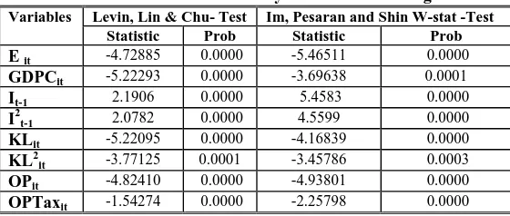
I test the stationarity of variables in the model. Therefore, I make the unit root test of Levin, Lin & Chu and Im, Pesaran & Shin W-stat to test for it. The results show that all variables are stationarity at level in tree regions (Tables 1-3).
Table 1: Variables Stationarity Tests in the EU Region
Variables Levin, Lin & Chu- Test Im, Pesaran and Shin W-stat -Test
Statistic Prob Statistic Prob
E it -4.72885 0.0000 -5.46511 0.0000 GDPCit -5.22293 0.0000 -3.69638 0.0001
It-1 2.1906 0.0000 5.4583 0.0000
Table 2: Variables Stationarity Tests in the Persian GULF Countrries Region
Variables Levin, Lin & Chu- Test Im, Pesaran and Shin W-stat -Test
Statistic Prob Statistic Prob
E it -4.76166 0.0000 -5.38136 0.0000
GDPCit 3.8916 0.0000 2.3100 0.0000
It-1 -3.37040 0.0004 -3.64995 0.0001
I2t-1 -2.76661 0.0028 -2.80495 0.0025
KLit -4.14437 0.0000 -4.42455 0.0000
KL2
it -4.27300 0.0000 -4.67313 0.0000
OPit -5.33756 0.0000 -5.22526 0.0000
OPTaxit 4.6516 0.0000 -3.45377 0.0003
Table 3: Variables Stationarity Tests in the North-South Region
Variables Levin, Lin & Chu- Test Im, Pesaran and Shin W-stat -Test
Statistic Prob Statistic Prob
E it -6.69888 0.0000 -7.66961 0.0000
GDPCit -4.25459 0.0000 -3.64145 0.0000
It-1 -2.35173 0.0093 -4.65037 0.0000
I2
t-1 -2.38577 0.0085 -3.89213 0.0000
KLit -6.58359 0.0000 -6.07613 0.0000
KL2
it -5.69339 0.0000 -5.74948 0.0000
OPit -3.63459 0.0000 -4.79467 0.0000
OPTaxit 4.66753 0.0000 -4.44529 0.0003
I employ different panel data procedures to avoid estimation problems, namely, autocorrelation and heteroskedasticity. Heteroskedasticity and autocorrelation arises from different countries characteristics. Therefore, I employ GLS for panel data to avert autocorrelation and heteroskedasticity. The different tests show that we have autocorrelation and heteroskedasticity in the Persian Gulf, EU and South-North countries regions (Tables 4-6-8).
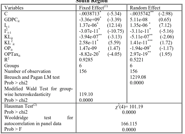
The coefficients OPTax are negative and significant in Persian Gulf,
EU and South-North countries regions, i.e. the policy of country’s net tax on dirty products spurs innovation which decreases the CO2 emission per capita
in these regions. Therefore, the Porter hypothesis is valid for the policy of net tax on dirty products in the Persian Gulf, EU and South-North countries
regions.
the CO2 emission per capita in the Persian Gulf, EU and South-North
countries regions (Tables 5-7-9)
Table 4: The Determinants of the CO2 Emission PER Capita in the EU Countries Region
Variables Fixed Effects(1)
Random Effect
C GDPCit It-1 I2 t-1 KLit KL2 it OPit OPTaxit R2 Groups
Number of observation Breusch and Pagan LM test Prob > chi2
Modified Wald Test for group-wise heteroskedasticity(3)
Prob > chi2
-.0038713* (-5.34) -3.36e+09* (-3.39) 1.37e-06* (12.14) -3.07e-11* (-10.75) -3.94e-07** (-3.13) 2.58e-11* (5.59) 1.47e-09 (1.47) -8.82e-20* (-4.05) 0.9285 6 156 338.80 0.0000 -.0035742** (-2.98) 5.11e-08 (0.65) 1.35e-06 *
(7.12) -3.11e-11* (-5.16) -5.11e-07** (-2.06) 1.41e-11*** (1.72) -1.94e-09* (-1.17) 2.97e-19** (1.95) 0.5221 6 156 121.08 0.0000
Hausman Test(2) Prob > chi2
Wooldridge test for autocorrelation in panel data
Prob > F
χ2
(4)= 101.19 0.0000
20.492 0.0062
Note: T-statistics are shown in parentheses. Significance at the 99%, 95% and 90%. confidence levels are indicated by * , **and ***, respectively.
The robust standard errors are White’s heteroskedasticity-corrected standard errors (1)The acceptation of model by the Hausman test.
(2)The hausman test tests the null hypothesis that the coefficients estimated by the efficient random effects estimator are the same as the ones estimated by the consistent fixed effects estimator. If they are (insignificant P-value, Prob>chi2 larger than .05) then it is safe to use random effects. If you get a significant P-value, however, you should use fixed effects.
(3) For FE regression model, the modified Wald test for groupwise heteroskedasticity is
used while the Woolridge test for autocorrelation in panel data (Ho: no autocorrelation) is applied.
Table 5: The Calculatition of Differents Elasticities in the EU Region
Scale elasticity -0.227
Technique elasticity 3.357
Composition elasticity -0.486
Table 6: The Determinants of the CO2 Emission PER Capita in the PersianGULF Countries Region
Variables Fixed Effect Random Effect(1)
C GDPCit It-1 I2 t-1 KLit KL2 it OPit OPTaxit R2 Groups
Number of observation Breusch and Pagan LM test Prob > chi2
Modified Wald Test for group-wise heteroskedasticity
Prob > chi2
.0162479 * (4.99) 6.04e-07*
(3.83) -4.74e-09 (-1.39) 5.88e-16 (1.61) 6.14e-07 (0.67) -7.76e-11 (-1.36) -.0027928 (-0.85) -4.02e-13 (-1.21) 0.9285
6 156
361.06 0.0000
.0005229 (0.24) 1.16e-06 *
(10.91) -2.24e-09 (-1.22) 4.22e-16 (1.26) 8.82e-07** (1.93) -1.06e-10* (-2.85) .0062802* (4.16) -2.31e-12* (-5.13) 0.5221 6 156 5.87 0.0000
Hausman Test(2) Prob > chi2
Wooldridge test for autocorrelation in panel data
Prob > F
χ2
(4)= 24.79 0.0000
20.395 0.0063
Note: T-statistics are shown in parentheses. Significance at the 99%, 95% and 90%
confidence levels are indicated by * , **and ***, respectively.
The robust standard errors are White’s heteroskedasticity-corrected standard errors (1)The acceptation of model by the Hausman test.
(2)The hausman test tests the null hypothesis that the coefficients estimated by the efficient random effects estimator are the same as the ones estimated by the consistent fixed effects estimator. If they are (insignificant P-value, Prob>chi2 larger than .05) then it is safe to use random effects. If you get a significant P-value, however, you should use fixed effects. (3) For FE regression model, the modified Wald test for groupwise heteroskedasticity is
used while the Woolridge test for autocorrelation in panel data (Ho: no autocorrelation)
is applied.
Table 7: The Calculatition of Different Elasticities in the Persian GULF Countries Region
Scale elasticity 0.692 Technique elasticity -0.100 Composition elasticity 0.220
Table 8: The Determinants of the CO2 Emission PER Capita in the North- South Region
Variables Fixed Effect(1) Random Effect C GDPCit It-1 I2 t-1 KLit KL2it OPit OPTaxit R2 Groups
Number of observation Breusch and Pagan LM test Prob > chi2
Modified Wald Test for group-wise heteroskedasticity
Prob > chi2
-.0038713* (-5.34) -3.36e+09* (-3.39) 1.37e-06* (12.14) -3.07e-11* (-10.75) -3.94e-07** (-3.13) 2.58e-11* (5.59) 1.47e-09 (1.47) -8.82e-20* (-4.05) 0.9285
6 156
119.10 0.0000
-.0035742** (-2.98) 5.11e-08 (0.65) 1.35e-06 * (7.12) -3.11e-11* (-5.16) -5.11e-07** (-2.06) 1.41e-11*** (1.72) -1.94e-09* (-1.17) 2.97e-19** (1.95) 0.5221
6 156 1219.08 0.0000
Hausman Test(2) Prob > chi2
Wooldridge test for autocorrelation in panel data
Prob > F
χ2(4)= 101.19
0.0000
166.115 0.0000
Note: T-statistics are shown in parentheses. Significance at the 99%, 95% and 90% confidence levels are indicated by * , **and ***, respectively.
The robust standard errors are White’s heteroskedasticity-corrected standard errors (1)The acceptation of model by the Hausman test.
(2)The hausman test tests the null hypothesis that the coefficients estimated by the efficient random effects estimator are the same as the ones estimated by the consistent fixed effects estimator. If they are (insignificant P-value, Prob>chi2 larger than .05) then it is safe to use random effects. If you get a significant P-value, however, you should use fixed effects. (3) For FE regression model, the modified Wald test for groupwise heteroskedasticity is used
while the Woolridge test for autocorrelation in panel data (Ho: no autocorrelation) is applied.
Table 9: The Calculatition of Different Elasticities in the North-South Region Scale elasticity 0.409
Technique elasticity -0.076 Composition elasticity -0.194
5- Conclusions
The comparison of empirical studies testing the porter hypothesis reveals that several levels need to be distinguished, to which the porter hypothesis can be applied. This concerns at least the firm, industry, country levels. Depending on which level is the focus of analysis, results may differ. Also, comparison of studies is hindered by the use of different measures for competitiveness and stringency of environmental regulation. In particular measurement of the latter seems to be particular difficult (in the absence of undisputed definitions) yet at the time crucial for the interpretation of results form empirical studies, which overall indicate a small positive effect.
In this paper we have tested an empirical model based on the ACT model in order to provide evidence of the relevance of the Porter and van der Linde hypothesis. Our equation is focus on the net tax on dirty products between very environmental policies.
Our empirical results show that a more stringent environmental regulation (country’s net tax on dirty products), as trade be libered, spurs innovation which decreases CO2 emission per capita in the Persian Gulf, EU
and the South-North regions. Therefore, the Porter hypothesis is valid for the
policy of net tax on dirty products in these regions. Also, our results show that trade liberalisation increases the CO2 emission per capita in the Persian
Gulf, EU and South-North countries regions.
References
1-Antweiler, W., B.R. Copeland, M.S. Taylor (1998), “Is free trade good for the environment?”, Discussion Paper, No. 98-11, Vancouver, Department of Economics, University of British Columbia.
2-Antweiler, W., B.R. Copeland, M.S. Taylor (2001), “Is Free Trade Good for the Environment?”, The American Economic Review, Vol. 91 (4), pp. 877-908.
3-Barucci, E., F., Gozzi (2001), “Technology adoption and accumulation in a vintage capital model”, Journal of Economics, 52, 159-188.
5-Cole, M.A. and R.J.R. Elliott (2003), "Do Environmental Regulations Influence Trade Patterns? Testing Old and New Trade Theories", World Economy, 26, 1163-1186.
6-Copeland, B.R., M.S. Taylor (1995), “Trade and transboundary pollution”, American Economic Review, 85 (4), 716–737.
7-Feichtinger, G., R.F. Hartl, P.M. Kort, V.M. Veliov (2002), “Anticipation effects of technological progress on capital accumulation: a vintage capital approach”, Working Paper, 272.
8-Frankel J.A. and A.K. Rose (2002), “Is Trade Good or Bad for the Environment? Sorting Out the Causality”, National Bureau of Economic Research Working Paper, No: 9201. Cambridge, MA.
9-Grether, J.-M., J. De Melo (2003), “Globalization and Dirty Industries: Do Pollution Havens Matter?”, NBER Working Paper n. 9776, Cambridge, MA, USA.
10-Grossman, G.M. and A.B. Krueger (1995), "Economic Growth and the Environment", Quarterly Journal of Economics, Vol. 110(2), pp. 353-77. 11-Grossman, G.M., & A.B. Krueger (1991), “Environmental impacts of a North American free trade agreement”, NBER Working Paper 3914, Cambridge MA. Later published as Grossman and Krueger (1994).
12-Hartl, R.F., P.M. Kort, V.M. Veliov, G. Feichtinger (2001), “Capital accumulation under technological progress and learning: a vintage capital approach”, Working Paper, 271.
13-Holtz-Eakin, D., T.M. Selden (1995), “Stoking the fires? CO2 emissions and economic growth”, Journal Public Econ, 57 (1), 85 – 101.
14-Jaffe, A. B., S. Peterson, P. Portney, and R. Stavins (1995), “Environmental Regulation and the Competitiveness of US Manufacturing: What Does the Evidence Tell Us?”, Journal of Economic Literature, 33(March): 132-163.
15-Kriström, B. (1999), “On a clear day, you might see the environmental Kuznets curve”, Camp Resources (Wilmington, NC), 12-13 August
16-Kriström, B. (2000), “Growth, employment and the environment”, Swedish Economic Policy Review, forthcoming.
18-Palmer, K. L., W. E. Oates, and P. R. Portney (1995), “Tightening Environmental Standards: The Benefit-Cost or the No-Cost Paradigm?”, Journal of Economic Perspectives, 9(4): 119-132.
19-Porter, M., (1991), “America’s green strategy”, Scientific American, 264, 96
20-Porter, M.E., C. van der Linde (1995), “Toward a New Conception of the Environment-Competitiveness Relationship”, Journal of Economic Perspectives, Vol. 9 (4), pp. 97-118.
21-Rennings, K., (1998), “Towards a Theory and Policy of Eco-Innovation - Neoclassical and Evolutionary Perspectives”, in ZEW Discussion Paper 98-24, Mannheim: Center for Economic Research (ZEW).