ISSN:2574 -1241
Spatial Modelling of Some Conditional Autoregressive
Priors in A Disease Mapping Model: the Bayesian
Approach
DOI: 10.26717.BJSTR.2019.14.002555
Davies Obaromi*
Department of Mathematics/Statistics, Kogi State Polytechnic, Lokoja, Nigeria
*Corresponding author: Davies Obaromi, Department of Mathematics/Statistics, Kogi State Polytechnic, Lokoja, Nigeria
Received: January 31, 2019 Published: February 12, 2019
Citation: Davies Obaromi. Spatial Modelling of Some Conditional Au-toregressive Priors in A Disease Map-ping Model the Bayesian Approach. Biomed J Sci & Tech Res 14(3)-2019. BJSTR. MS.ID.002555.
Abbreviations: BYM: Besag, York And Mollie, CAR: Conditional Autore-gressive, TB: Tuberculosis, INLA: Inte-grated Nested Laplace Approximation Method, DIC: Deviance Information Criterion, SAR: Simultaneously Au-toregressive Model, ETR: Electronic Tuberculosis Register
ARTICLE INFO abstract
The basic model usually used in disease mapping is the Besag, York and Mollie (BYM) model, which combines two random effects, a spatially structured and a spatially unstructured random effect. Bayesian Conditional Autoregressive (CAR) model is a disease mapping method that is commonly used for smoothening the relative risk of any disease as used in the Besag, York and Mollie (BYM) model. This model (CAR), which is also usually assigned as a prior to one of the spatial random effects in the BYM model, successfully uses information from adjacent sites to improve estimates for individual sites. However, it has been pointed out that there exist some unrealistic or counterintuitive consequences on the posterior covariance matrix of the CAR prior for the spatial random effects. In the conventional BYM (Besag, York and Mollie) model, the spatially structured and the unstructured random components cannot be seen independently, and which challenges the prior definitions for the hyperparameters of the two random effects. Therefore, the main objective of this study is to utilize some spatial CAR models for flexibility as applied to tuberculosis (TB) disease mapping. The extended Bayesian spatial CAR model is proved to be a useful and a little robust tool for disease modeling and as a prior for the structured spatial random effects because of the inclusion of an extra hyperparameter. A Bayesian modeling approach by the Integrated Nested Laplace Approximation method (INLA) is used to estimate model parameters and comparison was made by the deviance information criterion (DIC).
Introduction
Disease mapping can be described as a technique for the presentation and estimation of summary procedures of spatially observed health outcomes. The increased and improved handiness of georeferenced data and flexible computational software has increased in the application of disease mapping in the areas of epidemiology and public health [1,2]. Disease mapping can also be used to define the geographical disparity of diseases, to detect clustering of diseases and to produce diseases maps. Some authors have given a good number of statistical reviews on disease mapping [3-7]. The main and central model employed for a univariate disease mapping is the Besag, York and Mollie (BYM) model and was proposed by [8]. This model is a type of the generalized linear mixed effects model, which has two spatial random effects; one
which is spatially unstructured and modeled using a normal prior and another, a spatially structured random effect which is modeled by an intrinsic conditional autoregressive (CAR) prior.
shrink-age and spatial smoothing of the raw relative risk estimate, which gives a steadier estimate of the outline of underlying risk of disease than that given by the raw estimates. This technique effectively bor-rows information from neighboring areas other than from far away areas and smoothing local rates toward local neighboring values. This decreases the variance in the associated estimates and allows for the spatial effect of regional differences in State populations.
Conditional autoregressive (CAR) models are regularly used for describing the spatial variation of quantities of interest in the form of aggregates over subregions. These models have been used to an-alyze data in various capacities, such as in demography, economy, epidemiology and geography. The general objective of these spatial models is to show and quantify spatial relations present among the data, in specific terms, to quantify how quantities of interest differ with explanatory variables and to also to identify clusters of ‘hot spots. General versions of CAR models, a class of Gaussian Markov random fields, appear in [10-12]. CAR models have been broadly applied in spatial statistics to model observed data [13-16] as well as (unobserved) latent variables and spatially varying random ef-fects [17,18] CAR model was first introduced by [19] and the Hi-erarchical disease-mapping models based on CAR was studied by [20] These CAR models yield spatial dependence in the covariance structure as a function of a neighbor matrix W, and regularly a fixed unknown spatial correlation parameter. The conditional autore-gressive (CAR) and the intrinsic autoreautore-gressive models (ICAR) are extensively used as prior distributions for the structured random spatial effects in Bayesian models. However, some unrealistic or counterintuitive consequences on the prior covariance matrix or the posterior covariance matrix of the spatial random effects have been pointed out by some authors [21]. This study therefore seeks to propose, utilize and compare another latent Gaussian model, an extended CAR model, as a prior for this spatial dependency model for flexibility and better smoothing.
Epidemiological Data Sources
This is a retrospective secondary data source from Eastern Cape Province TB notification and survey data. All data used is an extract from the electronic tuberculosis register (ETR) records of TB cases from the twenty-four health sub-districts of the province including the two metropolitan municipalities. The data obtained was for the year 2014. This study was carried out in the Eastern Cape province of South Africa. The Province of the Eastern Cape is situated on the east coast of South Africa and lies between the Western Cape and KwaZulu-Natal provinces. The Northern Cape and Free State prov-inces, as well as Lesotho shares borders with this Province. The Eastern Cape Province boasts of amazing natural diversity, stretch-ing from the semi-arid Great Karoo to the forests of the Wild Coast. It also extends around the Keiskamma valley, the fertile Langkloof, and the mountainous southern Drakensberg region. The main fea-ture of the Eastern Cape is its amazing coastline adjoining the
In-The Province is situated at 32.2968°S and 26.4194°E of the country. The Eastern Cape is the second-largest province in South Africa by surface area and also the third-largest populated province with its capital in Bhisho. Port Elizabeth, East London, Grahamstown, Mtha-tha (previously Umtata), Graaf Reinet, Cradock and Port St Johns are the major towns and cities in the province. The province is di-vided into two metropolitan municipalities, and they are Buffalo City Metropolitan Municipality and Nelson Mandela Bay Metropol-itan Municipality. It has six district municipalities, and which are further subdivided into 37 local municipalities.
Modelling the Spatial Dependency Structure
Generally, it seems reasonable to assume that areas that are close in space show more similar disease burden than areas that are not close. To be “close” here means that we need to set up a neighbourhood structure. A well-known assumption is to regard areas i and j as neighbours if they have a common border, repre-sented here as i~j. This appears sensible if the regions are equally sized and organized in a regular pattern [3]. We further denote the set of neighbours of region i by δi and its size by nδi.
Review of Some Common Spatial Dependency Models
The BYM Model: The assumption of the Besag model adopts that a spatially structured component cannot take the limiting form that allows for no spatially structured variability. Hence, unstruc-tured random error or pure overdispersion within area i, will be modelled as spatial correlation, giving confusing parameter es-timates [22]. To address this issue, the Besag-York-Mollie (BYM) model [23] splits the regional spatial effect b into a sum of an un-structured and a un-structured spatial component, so that.
b
=
v
+
u
Here, (0, 1 )
v
v�ℵ
τ
−I accounts for pure overdispersion, while1
(0, u ) u�ℵ τ−Q−
is the Besag model whereby Q−
represents the gen-eralized inverse ofQ. The subsequent covariance matrix of b is
1 1
,
(
u v)
v uVar b
τ τ
=
τ
−I
+
τ
−Q
−Intrinsic CAR (Besag) Model: The simplest of the CAR prior is the intrinsic model suggested by [8], which is given as
(
)
1
1
1 1
1
| ~ i j, ,
n j
i n n
j j j ij
N ω φ ω ρ φ φ
τ ω
=
= =
∑
∑ ∑
i=1,...,n (3)
the lack of a parameter to regulate the strength of the spatial auto-correlation; if you multiplied ϕ by 10, then the precision τ, would decrease, but the spatial structure does not change. This implies that the intrinsic model is only practical in circumstances where the spatial autocorrelation in the data is strong; however, it is not practical for situations where there is a weak or moderate spatial autocorrelation across the study area because the model would have a tendency to produce an overly smooth estimated risk sur-face in these cases.
The Dean Model: [24] proposed a reparameterisation of the BYM model where
(
)
1 1 b
b φv φu
τ
= − + (4)
having covariance structure
(
,
)
1(
(
1
)
1)
b
Var b b
τ φ
=
τ
−−
φ
I
+
φ
Q
− (5) Equation (5) is a reparameterisation of the original BYM model, where τ_u^ (-1) =τ_b^ (-1) ϕ and τ_v^(-1) =τ_b^(-1) (1-ϕ) [25].A New Besag2 ICAR Model for the Structured Spatial Ef-fects: A modification of the Dean model in (2.42) was proposed by and which addresses both the identifiability and scaling issue of the BYM model. The model uses a scaled structured component μ_(i*) where τ is the precision matrix of the Besag ICAR model. The “Be-sag2” is one of the models in the latent Gaussian field. The Besag2 model is an extension to the Besag (ICAR) model above in (3.14).
Paramerisation of the Besag2 Model
Let the random vector z=(x1,…,xn) be the “Besag” model (ICAR), then the “Besag2” is the following extensions
x=
(
az z a, /)
(6)where a>0 is an additional hyperparameter and dim(x)=2n, and z is the same (a tiny additive noise) random vector.
Hyperparameters
This model has two hyperparameters θ= (θ1, θ2). The precision parameter τ is represented as
Q
1 log
=
tau
(7) And the prior is defined on θ1.The weight parameter a is signified as
θ =2 loga (8)
And the prior is defined on θ2. The precision defines how equal the two copies of z is. This new prior is a member of the class of a latent Gaussian (LGMs) markov random field models and would be
compared with the Besag ICAR, and the BYM models for flexibility and robustness.
Methods
Bayesian Modeling Approach
Bayesian analysis rests upon computing the posterior proba-bility distribution for model parameters. The posterior probaproba-bility distribution is the conditional probability distribution of the un-known parameters, given the observed data and weighted by the prior information. Bayesian modelling depends on the ability to compute posterior distributions in order to provide estimates for all the corresponding model parameters. Majority of these posteri-or distributions are straightfposteri-orward to calculate. Distributions with a conjugate prior typically have a posterior distribution which fol-lows a standard distributional form.
Bayesian Inference
The prior distribution is the distribution of the parameter(s) before any data is observed, that is,
(
)
p θ α│ .The prior distribution might not be easily determined. In this case, we can use the Jeffreys prior to obtain the posterior distribu-tion before updating them with newer observadistribu-tions.
The sampling distribution is the distribution of the observed data conditional on its parameters, i.e.
(
)
p X│
θ
This is also termed the likelihood, especially when viewed as a function of the parameter(s), sometimes written,
(
)
(
|)
. L θ│X = p X θThe marginal likelihood (sometimes also termed the evidence) is the distribution of the observed data marginalized over the pa-rameter(s),
( ) ( ) ( )
p X│α = ∫θ p X│θ p θ α│ dθ
The posterior distribution is the distribution of the param-eter(s) after taking into account the observed data. This is deter-mined by Bayes’ rule, which forms the heart of Bayesian inference
(
,)
(
(
) (
)
)
)/(
(
|)
)
( ) ( )p θ│X α = p X│θ pθ α│ p X α ∝p X│θ pθ α│
In many cases, however, the computation required is more complex and a more advanced method is essential to calculate the posterior distribution. These advanced approaches usually make use of some form of numerical simulation, generally by drawing a sample of parameter values from an approximation of the posteri-or distribution f( | )θ Y to allow estimation of the distributions of
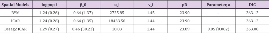
Table 1: Comparison of priors for the structured random effects model at 97.5% C.I without covariates.
Spatial Models logpop i β_0 u_i v_i pD Parameter, a DIC
BYM 1.24 (0.26) 0.64 (1.37) 2725.85 1.45 23.90 - 263.12
ICAR 1.24 (0.26) 0.64 (1.35) 18433.50 1.44 23.90 - 263.12
Besag2 ICAR 1.29 (0.27) 0.46 (30.23) 18.83 1.44 23.89 0.05 (0.002) 263.08
Parameter Estimation by The Integrated Nested Laplace
Approximation (INLA) Method
The marginal of the posterior are not always presented in closed form as a result of the non-Gaussian response variables. For such models, Markov chain Monte Carlo methods can be applied, but they are not without some complications, both in terms of con-vergence and in computational time. In some practical uses, the level of these problems is such that Markov chain Monte Carlo is basically not a suitable tool for monotonous analysis.
It is shown in that by using the integrated nested Laplace ap-proximation (INLA) method in its basic form, we can directly com-pute very accurate approximations to the posterior marginal. The key advantage of these approximations is simply computational, as MCMC algorithms need hours and days to run, while INLA provide more exact estimates in seconds and in minutes. Another benefit with INLA method is its generality, which makes it possible to ex-ecute Bayesian analysis in a programmed, streamlined way and to compute model comparison criteria and many predictive measures, so that models can be compared and the model under study can be tested. This method is also used where the model has a hidden Gaussian Markov Random field, with the parameters of interest be-ing latent variables which are not observed directly but are instead inferred from other observed variables.
Considering the following hierarchical model, ( )
i i
Y Poisson= µ
i
=
1,...,
n
log( ) T
i xi i
µ
=β
+θ
(9) Given that, φ=( ,..., )φ1 φn comprise a set of random effects, whichcan be considered as a group of latent variables. Let be the set of hyperparameters relating to, then the marginal posterior for each variable
φ
i is as follows:1
( | )i Y ω φ ( , | )Y d di
π φ =
∫ ∫
−π φ ω φ ω− (10)where,
φ
−1 is the vectorφ
with elementφ
i removed. This can be modified as( | )i Y ω ( | , ) ( | )i Y Y d
π φ =
∫
π φ ω π ω ω (11)INLA involves the construction of a nested approximation of (5), which requires approximations of and . Here can be approxi-mated using the following Laplace approximation
(
, ,Y)
π φ ωwhere π ̃_c (ϕ_i│ϕ,ω,Y) is termed the Gaussian approximation to the full conditional distribution of and is the mode of the full con-ditional distribution of for a given value of . The authors in propose using a Laplace estimate π φ ω( I | ,Y)of which takes the following form:
( ) ( ) ( ) ( ) ( )
~ ~
| , | , / | , , ) | *( , )
i i
LA Y Y G i i Y i i i
π− φ ω απ φ ω π− φ− φ ω− φ− − =φ− − ∧ φ ω− (13)
where π ̃_G (ϕ_(-i)│ϕ_i,ω,Y) is the Gaussian approximation to and as its modal value for a given
ω
.Although in most cases similar results will be obtained by MCMC and INLA inference, it should be noted that there are fun-damental differences in the way that posterior distributions are estimated. MCMC can sample directly from a joint posterior distri-bution, while INLA uses a closed form expression to estimate the marginal posterior distributions. For this study, we adopted the lat-ter and the analysis was carried out in R. Models comparison were carried out using the Deviance Information Criterion (DIC), which pools together a measure of fit and a measure of model complexity based on the effective number of parameters. Smaller values of DIC show a more fitting model [26].
Model Comparison
The comparison of numerous contending Bayesian models is usually a challenging task and needs special attention [27] Since the models used include sets of random effects, the Deviance Infor-mation Criterion (DIC) shall be used for comparison. It is defined as
, log
DIC = +D pd where D E− − = − L∧
where is given as the mean posterior deviance and pd rep-resents the actual number of parameters. When two or more mod-els are compared, the model with the least DIC value would be adopted. Similar to the BIC, this approach penalises models which have superfluous parameters, and favours approaches which pro-vide a sensible data fit while minimizing the amount of parameters. The best fitting model shall be the one with the smallest DIC value.
Statistical Analysis
Our working model is the usual BYM model which is a type of generalized linear mixed model (GLMM) with both fixed and ran-dom effects;
1
log k
i i i ik
y =
α
+ ∑=β
x +b (9)fects. For this analysis, the standard Besag, York and Mollie convo-lution model is adjusted with additive spatial random effects and then used to compare the priors for the structured random effect, u_i. An offset variable, log pop, of each region i, is used as a covariate in the model.
Model:
(
)
0 ; ~ , _ ~ \" "i i i i
logλ =Log pop +β + +v u v iid u i Besag ICAR
Three (3) multilevel models with only one covariate as an offset variable are hereby developed for comparison between the spatial models BYM, the intrinsic CAR and the new “Besag2” ICAR model with additive spatial random effects and given as:
Model 1:
(
)
0; ~ , _ ~
i i i i
log
λ
=
Log pop
+
β
+ +
v u v
iid u i BYM
Model 2:
(
)
0 ; ~ , _ ~i i i i
log
λ
=Log pop +β
+ +v u v iid u i BesagICAR Model 3:(
)
0 ; ~ , _ ~i i i i
logλ =Log pop +β + +v u v iid u i BesagICAR
Results
Figure 1: Posterior estimated spatial maps of the structured
random prior comparisons of BYM, Besag ICAR and the new “Besag2” ICAR spatial models respectively.
The results of a Bayesian disease-mapping analysis are pre-sented in the form of maps displaying the spatial patterns of the three different CAR models in Figure 1. Table 1 shows the deviance information criterion for the three spatial CAR models in which
the newly introduced two-parameter “Besag2” CAR model has the lesser deviance. For any model selection, deviance should be less and based on that, the Besag2 CAR model is fitted best out of the three models (Figure 2). Also, from the reparameterised “Besag2” ICAR model, which has the advantage of possessing two hyperpa-rameters over the Besag ICAR prior with only one hyperparameter, the posterior estimates of the new prior gave significantly r educed variances for the two spatial components, and especially for the structured spatial component (σ=18.83), thereby making it to be considered as the best fit model. In terms of model choice criteria by DIC values, the three models perform at least equally well with current parameterisations, but only the Besag2 ICAR model offers parameters that are clearly interpretable and with better precision. The comparative spatial maps of the BYM and the usual ICAR mod-els are very identical as shown in Figure 1. Spatial maps of ICAR and the new Besag2 ICAR models showed varying disease patterns when the two prior models were compared. The third model which utilized the new prior “Besag2” ICAR showed a better smooth and a more defined disease cluster and distribution. Also, the range of the posterior risks is reduced and better smoothed.
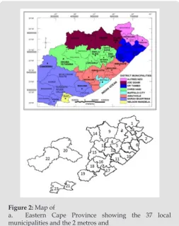
Figure 2: Map of
a. Eastern Cape Province showing the 37 local municipalities and the 2 metros and
b. Extracted map from R showing the 24 health sub-districts for the TB dataset.
Discussion
Autore-gressive (CAR) model which has only one precision hyperparame-ter, τ. This CAR model offers some shrinkage and spatial smoothing of the raw relative risk estimate, which gives a more stable estimate of the shape of the underlying risk of disease than that given by the raw estimates [28] Without suitable weighting that is characterized with the usual ICAR prior, the hyperparameter usually have no clear meaning and may be incorrectly interpreted. This sole parameter of this ICAR rest on the basic graph structure and is confused with the mixing parameter if the structured spatial effect is not correctly scaled. Also, it is not clear on how to select a prior distribution for this precision parameter. For lack of weighting, a fixed hyperprior for the precision parameter usually give diverse amount of smooth-ing if the graph on which given disease counts are observed is al-tered [29] Also, the commonly used hyperprior distributions in the traditional ICAR prior models usually induce overfitting, and will not permit to reduce to simpler models such as a constant risk sur-face or uncorrelated noise over space [30] The spatially structured random effect cannot be treated individually from the unstructured spatial random effect in the classical or frequentist BYM (Besag, York and Mollie) model. This makes the prior explanations for the hyperparameters of the two spatial random effects problematic and challenging [29].
However, the major objective is not only to optimize model choice criteria such as DIC values, but to offer a sensible model de-sign where all parameters have a clear de-significance and interpreta-tion. This new model however, parameterizes the BYM model and is also an extension of the Besag ICAR model, that leads to better pa-rameter control as the hyperpapa-rameters can be seen independently from each other. The main advantage of this novel “Besag2” ICAR model is that it permits for an intuitive parameter explanation and enables prior assignment. Also, the model is able to shrink towards a spatially unstructured risk for different disease prevalence. This shows that the Besag2 ICAR model does not overfit the parameter estimates. It is therefore acceptable, that the practical advantages in terms of interpretability and prior assignment makes the newly proposed Besag2 ICAR model in this study beneficial compared to existing models, and its usage is also recommended since its model criteria performance is better than existing approaches. The Be-sag2 ICAR model can be joined naturally with covariate data for use, or combined into a spatio-temporal setting [29].
Though, it will involve additional effort to allocate the vari-ance not only within the spatial components but overall model pa-rameters in the linear predictor. It should also be noted that the Besag2 ICAR model is not only remarkable within the context of disease mapping but also within other applications, such as genet-ics. Bayesian approaches provide suitable smoothing of the back-ground rates. Mapping the raw SMRs would present a confusing and distorting picture of the risk pattern, whereas in the Bayesian models, a good posterior relative risk is obtained in all the areas
context, are useful for smoothing disease relative risk estimates based on neighborhood structures.
Author Contribution
Davies Obaromi designed and formulated the study. Davies Obaromi drafted the manuscript, analyzed and interpreted the data.
Ethical Consideration
This study was carried out under the authorization and permis-sion of the Ethical committee of the University of Fort Hare, Alice, Eastern Cape, South Africa and approval of the Eastern Cape De-partment of Health, with ethical clearance reference number QIN-041SOBA01 and EC_2015RP24_398 respectively.
References
1. Rezaeian M, Dunn G, St Leger S, Appleby L (2007) Geographical Epidemiology Spatial Analysis and Geographical Information Systems: A Multidisciplinary Glossary. Journal of Epidemiology of Community Health. Volume 61(2): 98-102.
2. Everitt BS, Dunn G (2011) Applied Multivariate Analysis 2001 Arnold London. Statistical Methods in Medical Research 20: 49-68.
3. Wakefield J (2007) Disease mapping and spatial regression with count
data. Biostatistics 8(2): 158-183.
4. Clayton D, Bernardinelli L (1992) Bayesian methods for mapping disease risk: Geographical andenvironmental epidemiology methods for small-area studies. Oxford University Press Oxford.
5. Smans M, Esteve J (1997) Pratical approaches to disease mapping: Geographical and Environmental Epidemiology, Methods for Small area studies. Oxford University Press.
6. Bell B, Broemeling L (2000) A Bayesian Analysis of Spatial Processes with Application to Disease Mapping. Stat Med 19(7): 957-974.
7. Manda SM, Feltbower RG, Gilthorpe MS (2011) Review and empirical comparison of joint mapping of multiple diseases. Southern African Journal of Epidemiology and Infection 27(4): 169-182.
8. Besag J, York J, Mollie A (1991) Bayesian image restoration with two applications In spatial statistics (with discussion). Ann Inst Stat Math 43: 1-59.
9. Clayton D, Kaldor J (1987) Empirical Bayes stimates of age-standardized relative risks for use in disease mapping. Biometrics 43(3): 671-681.
10. Cressie NAC (1993) Statistics For Spatial Data. Wiley Interscience.
11. Banerjee S, Carlin BP, Gelfand AE (2004) Hierarchical Modelling and Analysis for Spatial Data. Chapman and Hall/CRC Florida USA.
12. Rue H, Held L (2005) Gaussian Markov Random Fields Theory and Applications.104of Monographs on Statistics and Applied Probability Chapman & Hall/CRC.
13. Cressie NA, Chan N (1989) Spatial Modelling of Regional Variables. Journal of the American Statistical Association 84 (40): 393-401.
14. Richardson S, Guihenneuc C, Lasserre V (1992) Spatial Linear Models with Autocorrelated Error Structure. The Statistician 41(5): 539-557.
15. Militino AF, Ugarte MD, Garcia Reinaldos L (2004) Alternative models for describing spatial dependence among dwelling selling prices. Journal of Real Estate Finance and Economics 29(2): 193-209.
16. Cressie N, Perrin O, Thomas Agnan C (2005) Likelihood-based estimation for Gaussian MRFs. Statistical Methodology 2(1): 1-16.
18. Pettitt AN, Weir IS, Hart AG (2002) A conditional autoregressive Gaussian process for irregularly spaced multivariate data with application to modelling large sets of binary data. Statistics and Computing 12(4): 353-367.
19. Besag J (1974) Spatial interaction and the statistical analysis of lattice systems. Journal of the Royal Statistical Society. Series B (Methodological) 36(2): 192-236.
20. Besag J, Kooperberg C (1995) On conditional and intrinsic autoregressions. Biometrika 82(4): 733-746.
21. Renato Assuncao, Elias Krainski (2009) Neighborhood Dependence In Bayesian Spatial Models. Biometrical Journal 51(5): 851-869.
22. Breslow N, Leroux B, Platt R (1998) Approximate hierarchical modelling of discrete data in epidemiology. Statistical Methods in Medical Research 7(1): 49-62.
23. Leroux BG, Lei X, Breslow N (1999) Estimation of disease rates in small areas: A new mixed model for spatial dependence. Statistical Models in Epidemiology the Environment and Clinical Trials 116: 179-192.
24. Dean C, Ugarte M, Militino A (2001) Detecting interaction between
random region and fixed age effects in disease mapping. Biometrics
57(1): 197-202.
25. Macnab YC (2011) On Gaussian Markov random fields and Bayesian
disease mapping. Statistical Methods in Medical Research 20(1): 49-68.
26. Spiegelhalter DJ, Best NG, Carlin BP (2002) Bayesian measures of model
complexity and fit. Journal of the Royal Statistical Society: Series B
(Statistical Methodology) 64(4): 583-639.
27. Kass R, Raftery A (1995) Bayes Factors. Journal of American Statistical Association 90(430): 773-795.
28. Venkatesan P, Srinivasan R, Dharuman C (2012) Bayesian Conditional Autoregressive Model for Mapping Tuberculosis Prevalence in India. International Journal of Pharmaceutical Studies and Research.
29. Andrea R, Sigrunn HS, Simpson D, Havard R (2016) An intuitive Bayesian spatial model for disease mapping that accounts for scaling.
30. Simpson DP, Rue H, Martins TG (2015) Penalising model component complexity: A principled practical approach to constructing priors.
Submission Link: https://biomedres.us/submit-manuscript.php
Assets of Publishing with us • Global archiving of articles
• Immediate, unrestricted online access • Rigorous Peer Review Process • Authors Retain Copyrights • Unique DOI for all articles
https://biomedres.us/
This work is licensed under Creative Commons Attribution 4.0 License ISSN: 2574-1241
DOI: 10.26717.BJSTR.2019.14.002555