Journal of Chemical and Petroleum Engineering, University of Tehran, Vol. 48, No.1, Jun. 2014, PP. 27-45 27
* Corresponding author: Tel: +98 9166674989 Email: [email protected]
Estimation of Binary Infinite Dilute Diffusion Coefficient
Using Artificial Neural Network
Majid Mohadesi*, Gholamreza Moradi and Hosnie-Sadat Mousavi
Chemical Engineering Department, Faculty of Engineering, Razi University,
Kermanshah, Iran
(Received 6 August 2013, Accepted 29 October 2013)
Abstract
In this study, the use of the three-layer feed forward neural network has been investigated for estimating of infinite dilute diffusion coefficient ( 12D ) of supercritical fluid (SCF), liquid and gas
binary systems. Infinite dilute diffusion coefficient was spotted as a function of critical temperature, critical pressure, critical volume, normal boiling point, molecular volume in normal boiling point, molecule diameter, Lennard-Jones’s (LJ) energy parameter, temperature and pressure. For each set of SCF, liquid and gas systems a three-layer network has been applied with training algorithm of Levenberg-Marquard (LM). The obtained results of models have shown good accuracy of artificial neural network (ANN) for estimating infinite dilute diffusion coefficient of SCF, liquid and gas binary systems with mean relative error (MRE) of 2.88 % for 231 systems containing 4078 data points (mean relative error for ANN model in SCF, liquid and gas binary systems are 3.00, 2.99 and 1.21 %, respectively).
Keywords
:
Artificial neural network, Binary mixture, Infinite dilute diffusion coefficient, Supercritical fluidIntroduction
Infinite dilute diffusion coefficient (
D12)
is one of the most important transport
properties. In which molecule 1 is solvent
and molecule 2 is solute, which each
molecule 2 is in an environment of pure
molecule 1. Concentration of molecule 2 is
up to 5 and perhaps 10 mole percent [1]. In
some of the industrial processes such as
extraction from SCFs, mixing of
concentrated liquids and gas systems in low
densities, systems can be supposed as
infinite dilute condition. For this reason
numerous equations have been presented for
estimating this property. These equations
are on the base of ideal gas, Enskog fluid,
hard sphere fluid, LJ fluid and real fluid
theories [2].
Although different theories and
semi-empirical correlations has been offered for
estimating of infinite dilute diffusion
coefficient, remarkable difference are
observed between results and real values. In
addition, each correlation has a high
accuracy only for special group of fluids.
Since last two decade using of neural
network has a wide spread application to
solve different problems of chemical
engineering
[3-15]. Recently Eslamloueyan and
Khademi [15] were investigated a
three-layer feed forward neural network to
estimate gases binary diffusion coefficient
in atmospheric pressure. In their suggested
model, temperature, critical temperature,
critical volume and molecular weight are
spotted as input data of the network.
In this work, three-layer feed forward
neural network was used for estimating
infinite dilute diffusion coefficient of binary
SCF, liquid and gas systems separately.
Results were shown good accuracy of
models in comparison with experimental
data and the other models.
1. Methodology
28 Journal of Chemical and Petroleum Engineering, University of Tehran, Vol. 48, No.1, Jun. 2014
1.1. Analyzing and using of data
In this work a large complex of data
were compiled that consists of 231 systems
and 4078 data points (binary mixtures of
SCF (111 systems/3277 points), binary
liquid (88 systems/549 points) and binary
gas mixtures (32 systems/252 points)). An
ANN was used for each one of SCF, liquid
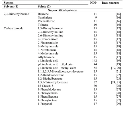
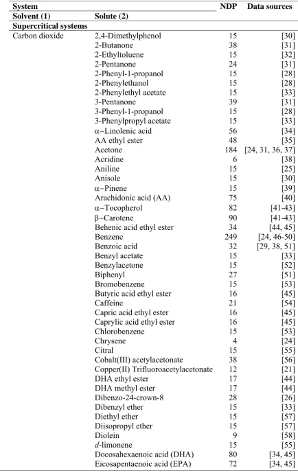
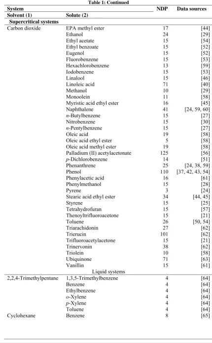
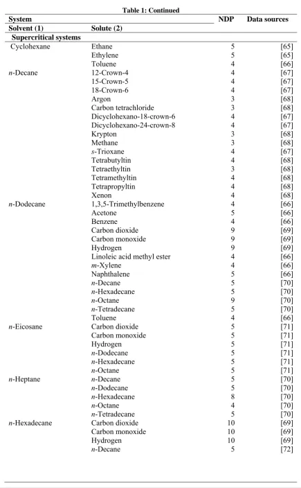
and gas systems. Table 1 shows the studied
systems, number of data point (NDP) and
sources of data. Three-fourths of data were
used for training of network and the rest
used for test. In these models infinite dilute
diffusion coefficient is spotted as a function
of molecular weight, critical properties,
normal boiling point, molar volume in
normal boiling point, molecule diameter, LJ
energy parameter, temperature and pressure:
P T k
ε σ
V T
V P T M k
ε
σ
V T V P T M f D
B LJ LJ bp bp
c c c B
LJ
LJ bp bp c c c
, , / , , ,
, , , , , /
, , , , , , ,
2 2
2 2
2 2 2 2 1
1 1 1 1 1 1 1
12
(1)
Table 1: Studied systems and data sources
System NDP Data sources
Solvent (1) Solute (2)
Supercritical systems
2,3-Dimethylbutane Benzene 11 [16]
Napthalene 9 [16]
Phenanthrene 11 [16]
Toluene 10 [16]
Carbon dioxide 1,3-Divinylbenzene 15 [17]
2,3-Dimethylaniline 15 [18]
2,6-Dimethylaniline 15 [18]
2-Bromoanisole 15 [17]
2-Fluoroanisole 15 [17]
2-Methylanisole 15 [18]
3-Nitrotoluene 15 [18]
4-Methylanisole 15 [18]
Allylbenzene 15 [17]
γ-Linolenic acid 142 [19]
γ-Linolenic acid ethyl ester 44 [19]
γ-Linolenic acid methyl ester 55 [19, 20]
1,1,1,5,5,5-Hexafluoroacetylacetone 15 [21]
1,2-Dichlorobenzene 15 [22]
1,2-Diethylbenzene 15 [23]
1,3,5-Trimethylbenzene 22 [24, 25]
15-Crown-5 30 [26]
1-Phenyldodecane 15 [27]
1-Phenylethanol 15 [28]
1-Phenylhexane 15 [27]
1-Phenyloctane 15 [27]
Estimation of Binary Infinite ….. 29
Table 1: Continued
System
NDP
Data sources
Solvent (1)
Solute (2)
Supercritical systems
Carbon dioxide
2,4-Dimethylphenol
15
[30]
2-Butanone
38
[31]
2-Ethyltoluene
15
[32]
2-Pentanone
24
[31]
2-Phenyl-1-propanol
15
[28]
2-Phenylethanol
15
[28]
2-Phenylethyl acetate
15
[33]
3-Pentanone
39
[31]
3-Phenyl-1-propanol
15
[28]
3-Phenylpropyl acetate
15
[33]
Linolenic acid
56
[34]
AA ethyl ester
48
[35]
Acetone
184 [24, 31, 36, 37]
Acridine
6
[38]
Aniline
15
[25]
Anisole
15
[30]
Pinene
15
[39]
Arachidonic acid (AA)
75
[40]
Tocopherol
82
[41-43]
Carotene
90
[41-43]
Behenic acid ethyl ester
34
[44, 45]
Benzene
249
[24, 46-50]
Benzoic acid
32
[29, 38, 51]
Benzyl acetate
15
[33]
Benzylacetone
15
[52]
Biphenyl
27
[51]
Bromobenzene
15
[53]
Butyric acid ethyl ester
16
[45]
Caffeine
21
[54]
Capric acid ethyl ester
16
[45]
Caprylic acid ethyl ester
16
[45]
Chlorobenzene
15
[53]
Chrysene
4
[24]
Citral
15
[55]
Cobalt(III) acetylacetonate
38
[56]
Copper(II) Trifluoroacetylacetonate
12
[21]
DHA ethyl ester
17
[44]
DHA methyl ester
17
[44]
Dibenzo-24-crown-8
28
[26]
Dibenzyl ether
15
[33]
Diethyl ether
15
[57]
Diisopropyl ether
15
[57]
Diolein
9
[58]
d-limonene
15
[55]
Docosahexaenoic acid (DHA)
80
[34, 45]
30 Journal of Chemical and Petroleum Engineering, University of Tehran, Vol. 48, No.1, Jun. 2014
Table 1: Continued
System NDP Data sources
Solvent (1) Solute (2)
Supercritical systems
Carbon dioxide EPA methyl ester 17 [44]
Ethanol 24 [29]
Ethyl acetate 15 [54]
Ethyl benzoate 15 [52]
Eugenol 15 [52]
Fluorobenzene 15 [53]
Hexachlorobenzene 13 [59]
Iodobenzene 15 [53]
Linalool 15 [46]
Linoleic acid 71 [40]
Methanol 10 [29]
Monoolein 11 [58]
Myristic acid ethyl ester 16 [45]
Naphthalene 41 [24, 59, 60]
n-Butylbenzene 15 [27]
Nitrobenzene 15 [30]
n-Pentylbenzene 15 [27]
Oleic acid 19 [58]
Oleic acid ethyl ester 5 [58]
Oleic acid methyl ester 19 [58]
Palladium (II) acetylacetonate 125 [56]
p-Dichlorobenzene 14 [51]
Phenanthrene 25 [24, 38, 59]
Phenol 110 [37, 42, 43, 54]
Phenylacetic acid 16 [61]
Phenylmethanol 15 [28]
Pyrene 3 [24]
Stearic acid ethyl ester 34 [44, 45]
Styrene 15 [25]
Tetrahydrofuran 15 [57]
Thenoyltrifluoroacetone 15 [21]
Toluene 26 [50, 54]
Triarachidonin 27 [62]
Trierucin 101 [62]
Trifluoroacetylacetone 15 [21]
Trinervonin 38 [62]
Triolein 10 [58]
Ubiquinone 71 [63]
Vanillin 15 [61]
Liquid systems
2,2,4-Trimethylpentane 1,3,5-Trimethylbenzene 4 [64]
Benzene 4 [64]
Ethylbenzene 4 [64]
o-Xylene 4 [64]
p-Xylene 4 [64]
Toluene 4 [64]
Estimation of Binary Infinite ….. 31
Table 1: Continued
System NDP Data sources
Solvent (1) Solute (2)
Supercritical systems
Cyclohexane Ethane 5 [65]
Ethylene 5 [65]
Toluene 4 [66]
n-Decane 12-Crown-4 4 [67]
15-Crown-5 4 [67]
18-Crown-6 4 [67]
Argon 3 [68]
Carbon tetrachloride 3 [68]
Dicyclohexano-18-crown-6 4 [67]
Dicyclohexano-24-crown-8 4 [67]
Krypton 3 [68]
Methane 3 [68]
s-Trioxane 4 [67]
Tetrabutyltin 4 [68]
Tetraethyltin 3 [68]
Tetramethyltin 4 [68]
Tetrapropyltin 4 [68]
Xenon 4 [68]
n-Dodecane 1,3,5-Trimethylbenzene 4 [66]
Acetone 5 [66]
Benzene 4 [66]
Carbon dioxide 9 [69]
Carbon monoxide 9 [69]
Hydrogen 9 [69]
Linoleic acid methyl ester 4 [66]
m-Xylene 4 [66]
Naphthalene 5 [66]
n-Decane 5 [70]
n-Hexadecane 5 [70]
n-Octane 9 [70]
n-Tetradecane 5 [70]
Toluene 4 [66]
n-Eicosane Carbon dioxide 5 [71]
Carbon monoxide 5 [71]
Hydrogen 5 [71]
n-Dodecane 5 [71]
n-Hexadecane 5 [71]
n-Octane 5 [71]
n-Heptane n-Decane 5 [70]
n-Dodecane 5 [70]
n-Hexadecane 8 [70]
n-Octane 4 [70]
n-Tetradecane 5 [70]
n-Hexadecane Carbon dioxide 10 [69]
Carbon monoxide 10 [69]
Hydrogen 10 [69]
32 Journal of Chemical and Petroleum Engineering, University of Tehran, Vol. 48, No.1, Jun. 2014
Table 1: Continued
System NDP Data sources
Solvent (1) Solute (2)
Supercritical systems
n-Hexadecane n-Dodecane 5 [72]
n-Octane 10 [72]
n-Tetradecane 5 [72]
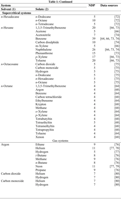
n-Hexane 1,3,5-Trimethylbenzene 20 [66, 73]
Acetone 5 [66]
Acetonitrile 7 [74]
Benzene 39 [64, 66, 73, 74]
Carbon disulphide 10 [74]
m-Xylene 5 [66]
Naphthalene 26 [66, 73, 74]
Phenanthrene 15 [73]
p-Xylene 17 [66, 73]
Toluene 20 [66, 73]
n-Octacosane Carbon dioxide 5 [75]
Carbon monoxide 5 [75]
Hydrogen 5 [75]
n-Dodecane 5 [75]
n-Hexadecane 5 [75]
n-Octane 5 [75]
n-Octane 1,3,5-Trimethylbenzene 4 [64]
Argon 4 [68]
Benzene 4 [64]
Carbon tetrachloride 4 [68]
Ethylbenzene 4 [64]
Krypton 4 [68]
Methane 4 [68]
o-Xylene 4 [64]
p-Xylene 4 [64]
Tetrabutyltin 4 [68]
Tetraethyltin 5 [68]
Tetramethyltin 4 [68]
Tetrapropyltin 4 [68]
Toluene 4 [64]
Xenon 4 [68]
Gas systems
Argon Ethane 9 [76]
Helium 11 [77, 78]
Hydrogen 5 [77]
i-Butane 8 [76]
Methane 9 [76]
n-Butane 8 [76]
Neon 11 [77, 79]
Propane 9 [76]
Carbon dioxide Helium 7 [80]
Hydrogen 7 [80]
Carbon monoxide Helium 7 [80]
Estimation of Binary Infinite ….. 33
Table 1: Continued
System NDP Data sources
Solvent (1) Solute (2)
Supercritical systems
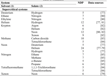
Deuterium Hydrogen 5 [77]
Ethane Nitrogen 7 [80]
Ethylene Nitrogen 7 [80]
Helium Hydrogen 12 [77, 81]
Krypton Argon 6 [82]
Helium 6 [82]
Neon 12 [80, 82]
Xenon 9 [82]
Methane Carbon dioxide 10 [83]
Tetrachloroethene 5 [84]
Neon Deuterium 5 [77]
Helium 24 [77-79]
Hydrogen 5 [77]
Nitrogen Ethane 7 [85]
Methane 7 [85]
n-Butane 5 [85]
Propane 6 [85]
Tetrafluoromethane 1,1,1-Trichloroethane 5 [84]
Tetrachloroethene 5 [84]
Xenon Neon 6 [79]
Critical properties (critical temperature,
critical pressure and critical volume) and
molecular descriptors are available in
literature [2], which estimated by several
equations. In Table 2 variation range of
each parameter (input data) and infinite
dilute diffusion coefficient (output data) are
summarized for SCF, liquid and gas
systems.
1.2. Neural network training
After determination of input data, ANN
was designed. In this case a three-layer feed
forward network has been used. Number of
neurons in hidden layer should has a
minimum value and if training error of
network with these number of neurons does
not have expected value, number of neurons
is increased one by one to achieve desired
value [86]. By applying neural network for
infinite dilute diffusion coefficient of SCF,
liquid and gas systems and changing
number of neurons in hidden layer, number
of optimal neurons was found in hidden
layer as 21, 19 and 18, respectively (attend
to Table 3). In these models, tansig transfer
function in hidden layer and purelin transfer
function in output layer were used which
are defined as follow:
χχ χχe e
e e
χ
f
tansig
(2)
χ χfpurelin
(3)
Also output of one neuron is computed
by following equation:
m
k
OL j k n
i
HL j i HL ji OL
jk
j f w f w x b b
O
1 1
tansig purelin
(4)
For training of data, neural network
algorithm of LM [87-89] was used.
Performance function of this algorithm is
MRE (
i NDP
i
calc D D
D NDP
MRE
1
. exp 12 . exp 12 .
12 /
/
100
),
34 Journal of Chemical and Petroleum Engineering, University of Tehran, Vol. 48, No.1, Jun. 2014
Table 2: Variations range of input and output of neural network
Property Supercritical systems Liquid systems Gas systems
Minimum Maximum Minimum Maximum Minimum Maximum
g/mol
1
M 44.01 86.18 84.16 394.77 4.00 131.30
K1
c
T 304.10 500.00 507.50 864.27 5.19 305.40
MPa
1
c
P 3.13 7.38 0.66 4.07 0.23 7.38
cm3/mol
1
c
V 93.90 358.00 308.00 1603.50 41.60 148.30
K1
bp
T 194.70 331.10 341.90 704.75 4.25 194.70
cm3/mol
1
bp
V 33.28 135.31 115.57 651.26 14.18 53.73
A
1
LJ
σ 3.58573 5.60165 5.32769 9.23375 2.73350 4.17576
εLJ /kB
1 K 241.48 397.05 403.00 686.31 4.12 830.49
g/mol
2
M 32.04 1137.91 2.02 460.61 2.02 165.83
K2
c
T 412.85 1601.10 33.00 1357.66 5.19 620.20
MPa
2
c
P 0.25 8.09 1.25 7.90 0.23 7.38
cm3/mol
2
c
V 118.00 3081.54 64.30 1210.75 41.60 289.60
K2
bp
T 299.15 1229.05 20.30 1077.88 4.25 394.40
cm3/mol
2
bp
V 42.28 1291.44 22.38 485.16 14.18 108.35
A
2
LJ
σ 3.86945 11.48007 3.16052 8.40827 2.73350 5.21941
εLJ /kB
2 K 4.12 1271.42 26.21 1078.11 4.12 830.49
KT 288.35 548.20 101.80 567.00 76.60 4262.00
MPa
P 5.35 40.11 0.101 385.600 0.101 0.101
cm /s
104 2
12
D 0.28 6.44 0.04 11.80 0.04×10⁴ 10.80×10⁴
2. Results and discussion
Results of determination of the optimal
number of neurons in hidden layer for SCF,
liquid and gas are presented in Table 3.
According to Table 3 the best neural
networks for SCF, liquid and gas systems
has 21, 19 and 18 neuron in hidden layer,
respectively. As it presented in Table 3
MRE of test data for SCF, liquid and gas
systems are 3.49, 2.60 and 2.38 %,
respectively.
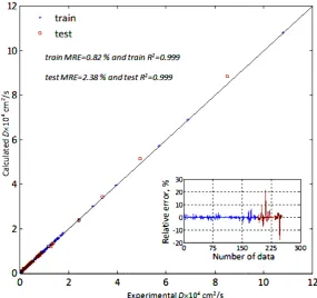
Figure 1 shows a correlation between
results of training and test data of neural
network and experimental data for SCF.
Also in this Figure percent of relative error (
exp.12 . exp 12 .
12 /
100
RE Dcalc D D
) for each
training and test data has been shown.
Figures 2 and 3 show the similar results for
liquid and gas systems, respectively. As it
can be observed from Figures 1 to 3, there
exist a good correlation between
experimental data and neural network
models output.
Estimati
Table
No
on of Binary In
e 3: Determin
o. of neurons
9 10 11 12 13 14 15 16 17 18 19 20 21 22 23 Figure 1: nfinite …..
ning of optim
train s Supercri
4.29 4.02 3.82 3.81 3.30 3.23 3.48 3.19 3.39 3.41 3.09 3.20 2.85 2.91 2.90 Comparison
mal number of
test tota itical system
4.33 4.30 4.43 4.11 4.37 3.95 4.28 3.92 4.26 3.52 3.76 3.36 4.16 3.64 5.08 3.62 5.80 3.94 3.93 3.53 3.59 3.21 3.65 3.30
3.49 3.00
3.94 3.15 4.52 3.28
between calc coe
f neuron in h
al train
ms Liq
0 5.82 1 4.92 5 3.86 2 4.28 2 3.81 6 4.07 4 4.44 2 3.16 4 3.32 3 5.67 1 3.12
0 3.68
0 3.42
5 3.19 8 3.57
culated and e efficient for S
hidden layer f MRE
test tot quid systems 5.98 5.8 4.43 4.8 3.43 3.7 4.03 4.2 3.46 3.7 3.54 3.9 4.28 4.4 2.94 3.1 2.66 3.1 5.04 5.5 2.60 2.9 3.58 3.6 2.67 3.2 2.74 3.0 3.04 3.4 experimental SCF
for SCF, liqu
al train
s G
86 0.89 80 1.08 75 0.96 21 0.71 72 0.96 94 0.96 40 0.97 11 0.84 16 0.84 51 0.82
99 0.95
66 0.91 23 0.82 08 0.73 44 0.83
infinite dilut
id and gas sy
n test to
Gas systems
5.88 2 2.37 1 2.71 1 11.12 3 9.50 3 3.78 1 4.22 1 3.03 1 2.67 1
2.38 1
3.87 1 2.79 1 4.50 1 6.97 2 3.37 1
36 J
Figure 2:
Figure 3:
Journal of Chem
Comparison
Comparison
mical and Petro
between calc coef
between calc co
oleum Engineer
culated and e fficient for liq
culated and e oefficient for g
ring, University
experimental quid
experimental gas
y of Tehran, Vo
infinite dilut
infinite dilut
l. 48, No.1, Jun
te diffusion
te diffusion
Estimation of Binary Infinite ….. 37
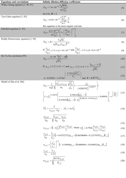
Table 4: Correlations and equations for infinite dilution diffusion coefficients Infinite dilution diffusion coefficients
Equations and correlations
(5) 6 . 0 2 , 1 1 8
12 7.4 10
bp
V
η
M T
D
Wilke-Chang equation [1, 90, 91]
for CO21
(6) 1 488 . 0 2 , 267 . 0 1 , 8
12 8.93 10 ηT
V V D bp bp
Tyn-Calus equation [1, 92]
this equation is for most organic solvents
(7) 3 / 2 2 , 1 , 3 / 1 3 , 1 8 12 3 1 10 2 . 8 bp bp bp V V V η T D
Scheibel equation [1, 93]
(8)
1/32 , 1 , 1 1 12 bp bp V V η M T β
D
Reddy-Doraiswamy equation [1, 94]
(9)
If 8
2 , 1 , 10 10 5 .
1
β
V V
bp
bp and 8
2 , 1 , 10 5 . 8 5 .
1
β V V bp bp (10)
2 1 7 12 10 M T B V A D k He-Yu-Su correlation [95]
(11) If ρr,11.2k1 and
1 1 , 1 , 2 . 1 1 2 . 1 M ρ k
ρr r
(12)
,1
1 , 1 75832 . 0 6736 . 1 29263 . 0 c c P V M e
A and B0.077Tc,1
(13)
12 12 12 2 41054 . 0 400152 . 0 12 12 12 126978 . 0 12 165877 . 0 12 12 12 12 1 , 12 2 , 12 12 68856 . 0 1 539292 . 0 1 596103 . 0 1 029079 . 1 1 8 3 T ρ ρ LJ LJ e T ρ ρ ρ T ρ ρ T m ε σ π D Model of Zhu el al. [96](14) 3 12 1 12 , 12
12 ε T/k , ρ ρσ
T B LJ (15) B LJ B LJ B LJ k ε k ε k
ε12, 1, 2,
(16)
1 12
1, 2 2, ,12LJ d LJ LJ
σ σ
k
σ where
LJ LJ LJ LJ d σ σ σ σ k , 2 , 1 , 1 , 2
12 0.7926
(17)
,1 ,1 ,1
1 ,
1 , ,
1 1 0.47527332 0.06300484 0.12374707 r r r c c B
LJ ρ ρ T
T T k ε (18)
,1 ,1 ,1
2 / 1 1 , 1 , ,
1 1 0.368868 r 0.0000694 0.01089228 r r c
c
LJ ρ ρ T
38 Journal of Chemical and Petroleum Engineering, University of Tehran, Vol. 48, No.1, Jun. 2014
Table 4: Continued Infinite dilution diffusion coefficients Equations and correlations
(21)
V VD
TB
D12 1
Dymond-Hildebrand-Batschinski free-volume expression [97, 98, 99]
(22) S
R B LJ ξ k Tξ
D , 12 , 12 ,
12
Real fluid theory [2]
(23)
12 , 12 12 2 , 12 1 ,12 83 2 F
σ g T k m π σ ρ
ξ R eff B eff
(24) 5 . 1 12 12 2 , 12 1 ,
12 38 2 0.4
T T k m π σ ρ
ξ S eff B
(25)
1/2 1/6 12, 12 ,
12 1.1532 1 1.8975
σ T
σ eff LJ
Table 5: Mean relative error for SCF, liquid and gas systems
System NDPa NDPb NSa NSb ANN Eq. (22) Eq. (21) Eq. (13) Eq. (10) Eq. (5) Eq. (6) Eq. (7) Eq. (8)
MRE
Supercritical 3277 3297 111 111 3.00 4.16 4.02 40.34 7.84 12.77 15.93 16.71 76.16 Liquid 549 548 88 87 2.99 5.66 5.83 38.56 - 43.85 44.19 80.98 45.39 Gas 252 251 32 28 1.21 1.83 2.01 43.30 - - - - - Total 4078 4096 231 226 2.88 4.22 4.14 40.28 7.83 17.20 19.96 25.87 71.77
a NDP and NS for ANN model. b NDP and NS for literature [2].
The minimum and maximum relative
errors by ANN are 0.1 %
(n-Octacosane-Carbon dioxide liquid system and (n-Octacosane-Carbon
monoxide-Helium gas system) and 9.73 %
(Carbon dioxide-Acridine SCF system).
Number of data of carbon dioxide-Acridine
system are 6 which in comparison with
other supercritical systems is a low value.
So probability of using these data by ANN
comes down and for estimating of infinite
dilute diffusion coefficient, ANN model
utilizes other substances data that have
similar properties to Acridine and this
subject caused low accuracy estimation.
Also total results are available in Table 5.
As shown in this table the MRE for ANN in
SCF, liquid and gas systems is 3.00, 2.99
and 1.21 %, respectively and average of
total error is 2.88 %.Total relative error for
Eqs. (5)-(8) are changed from 17.2 to 71.77
% (see Table 5). Eq. (10) that is used just
for SCF has a MRE=7.83 %, and Eq. (13)
has a poor results (MRE=40.28 %). Eqs.
(22) (Real fluid theory) and (21) have a
remarkable accuracy and MRE of 4.22 and
4.18 %, respectively.
3. Conclusions
In this work, artificial neural
network models were investigated for
estimation of infinite dilute diffusion
coefficient of binary SCF (111
systems/3277 points), liquid (88
systems/549 points) and gas (32
systems/252 points) systems. For each one
of SCF, liquid and gas systems a three-layer
feed forward neural network with train
algorithm of LM was used. In hidden and
output layers, transfer function of ‘tansig’
and ‘purelin’ were used, respectively. By
applying each one of the networks on
three-fourths of data, optimal number of neurons
in hidden layer for SCF, liquid and gas
systems is 21, 19 and 18, respectively.
Calculation results are shown high accuracy
of neural network models for SCF, liquid
and gas systems by MRE equal to 3.00, 2.99
and 1.21 %, respectively.
Nomenclature
A
parameter in Eq. (10)
B
parameter in Eqs. (10) and (21)
j
b
bias of
jth neuron
D
tracer diffusion coefficient,
cm2/sEstimation of Binary Infinite ….. 39
f
transfer function
σg
radial distribution function at contact
k
parameter in Eq. (10)
12
k
binary interaction parameter
d
k12
interaction parameter in Eq. (15)
Bk
Boltzmann constant,
K s / cm g. 10 380658 .1 16 2 2
M
molecular weight,
g/molm
mass of a molecule,
gNS
number of systems
jO
output of
jth neuron
Ppressure,
MPaT
temperature,
KV
molar volume,
cm3/molD
V
parameter in Eq. (21),
cm3/mol jiw
synaptic weight corresponding to
ith synapse
jth neuron
jk
w
synaptic weight corresponding to
kth synapse
jth neuron
ix i
th input signal to
jth neuron
Greek letters
β
parameter in Eq. (8)
χ
input value of neural network
B
k
ε/
Lennard–Jones energy parameter,
K dimensionless association factor of
the solvent
η
viscosity,
cPρ
density number,
cm-1 σmolecular diameter,
cmξ
friction coefficient
Subscripts
1
solvent
2
solute
12
binary property
bp
boiling point
c
critical property
eff
effective hard sphere diameter
LJ
Lennard–Jones fluid
R
repulsive contribution
r
reduced property
S
soft attractive contribution
Superscripts
reduced quantity
HL
hidden layer
OL
output layer
References
:
1- Reid, R.C., Prausnitz, J. M. and Poling, B.E. (2001). The Properties of Gases and Liquids. 5th. Ed.
McGraw-Hill Pub. Co., New York.
2- Magalhaes, A.L., Da Silva, F.A. and Silva, C.M. (2011). “New models for tracer diffusion coefficients of hard sphere and real systems: Application to gases, liquids and supercritical fluids.” J. Supercrit. Fluids, Vol. 55, pp. 898–923.
3- Bhat, N. and McAvoy, T.J. (2000). “Use of neural nets for dynamic modeling and control of chemical process systems.” Comput. Chem. Eng., Vol. 14, pp. 573-583.
4- Pollard, J.F., Broussard, M.R., Garrison, D.B. and San, K.Y. (1992). “Process identification using neural networks.” Comput. Chem. Eng., Vol. 16, pp. 253-270.
5- Psichogios, D.C. and Ungar, L.H. (1992). “A hybrid neural network-first principles approach to process modeling.” AIChE J., Vol. 38, pp. 1499-1511.
6- Wang, H., Oh, Y. and Yoon, E.S. (1998). “Strategies for modeling and control of nonlinear chemical processes using neural networks.” Comput. Chem. Eng., Vol. 22, pp. 823-826.
7- Molga, E. and Cherbanski, R. (1999). “Hybrid first-principle-neural network approach to modeling of the liquid-liquid reacting system.” Chem. Eng. Sci., Vol. 54, pp. 2467-2473.
40 Journal of Chemical and Petroleum Engineering, University of Tehran, Vol. 48, No.1, Jun. 2014
9- Kito, S., Satsuma, A., Ishikura, T., Niwa, M., Murakami, Y. and Hattori, T. (2004). “Application of neural network to estimation of catalyst deactivation in methanol conversion.” Catal. Today, Vol. 97, pp. 41-47. 10- Papadokonstantakis, S., Machefer, S., Schnitzleni, K. and Lygeros, A.I. (2005). “Variable selection and data
pre-processing in NN modeling of complex chemical processes.” Comput. Chem. Eng., Vol. 29, pp. 1647-1659.
11- Omata, K., Nukai, N. and Yamada, M. (2005). “Artificial neural network aided design of a stable Co-MgO catalyst of high-pressure dry reforming of methane.” Ind. Eng. Chem. Res., Vol. 44, pp. 296-301.
12- Himmelblau, D., (2008). “Accounts of experiences in the application of artificial neural networks in chemical engineering.” Ind. Eng. Chem. Res., Vol. 47, pp. 5782-5796.
13- Eslamloueyan, R. and Khademi, M.H. (2009). “Estimation of thermal conductivity of pure gases by using artificial neural networks.” Int. J. Thermal Sci., Vol. 48, pp. 1094–1101.
14- Eslamloueyan, R. and Khademi, M.H. (2009). “Using artificial neural networks for estimation of thermal conductivity of binary gaseous mixtures.” J. Chem. Eng. Data, Vol. 54, pp. 922–932.
15- Eslamloueyan, R. and Khademi, M.H. (2010). “A neural network-based method for estimation of binary gas diffusivity.” Chemom. Intell. Lab. Syst., Vol. 104, pp. 195–204.
16- Sun, C.K.J. and Chen, S.H. (1985). “Diffusion of benzene, toluene, naphthalene, and Phenanthrene in supercritical dense 2,3-dimethylbutane.” AIChE J., Vol. 31, pp. 1904–1910.
17- Suarez-Iglesias, O., Medina, I., Pizarro, C. and Bueno, J.L. (2007). “Diffusion coefficients of 2-fluoroanisole, 2-bromoanisole, allylbenzene and 1,3-divinylbenzene at infinite dilution in supercritical carbon dioxide.” Fluid Phase Equilib., Vol. 260, pp. 279–286.
18- Pizarro, C., Suarez-Iglesias, O., Medina, I. and Bueno, J.L. (2009). “Binary diffusion coefficients for 2,3-dimethylaniline, 2,6-2,3-dimethylaniline, 2-methylanisole, 4-methylanisole and 3-nitrotoluene in supercritical carbon dioxide.” J. Supercrit. Fluids, Vol. 48, pp. 1–8.
19- Kong, C.Y., Withanage, N.R.W., Funazukuri, T. and Kagei, S. (2006). “Binary diffusion coefficients and retention factors for γ-linolenic acid and its methyl and ethyl esters in supercritical carbon dioxide.” J. Supercrit. Fluids, Vol. 37, pp. 63–71.
20- Funazukuri, T., Hachisu, S. and Wakao, N. (1991). “Measurements of binary diffusion coefficients of C16–
C24 unsaturated fatty acid methyl esters in supercritical carbon dioxide.” Ind. Eng. Chem. Res., Vol. 30, pp.
1323–1329.
21- Yang, Y.N. and Matthews, M.A. (2001). “Diffusion of chelating agents in supercritical CO2 and a predictive
approach for diffusion coefficients.” J. Chem. Eng. Data, Vol. 46, pp. 588–595.
2 Gonzalez, K.M., Bueno, J.L. and Medina, I. (2002). “Measurement of diffusion coefficients for 2-nitroanisole, 1,2-dichlorobenzene and tert-butylbenzene in carbon dioxide containing modifiers.” J. Supercrit. Fluids, Vol. 24, pp. 219–229.
23- Pizarro, C., Suarez-Iglesias, O., Medina, I. and Bueno, J.L. (2007). “Using supercritical fluid chromatography to determine diffusion coefficients of 1,2-diethylbenzene, 1,4-diethylbenzene, 5-tert-butyl-m-xylene and phenylacetylene in supercritical carbon dioxide.” J. Chromatogr., A, Vol. 1167, pp. 202–209. 24- Sassiat, P.R., Mourier, P., Caude, M.H. and Rosset, R.H. (1987). “Measurement of diffusion coefficients in
Estimation of Binary Infinite ….. 41
25- Gonzalez, L.M., Suarez-Iglesias, O., Bueno, J.L., Pizarro, C. and Medina, I. (2007). “Limiting binary diffusivities of aniline, styrene, and mesitylene in supercritical carbon dioxide.” J. Chem. Eng. Data, Vol. 52, pp. 1286–1290.
26- Kong, C.Y., Takahashi, N., Funazukuri, T. and Kagei, S. (2007). “Measurements of binary diffusion coefficients and retention factors for dibenzo-24-crown-8 and 15-crown-5 in supercritical carbon dioxide by chromatographic impulse response technique.” Fluid Phase Equilib., Vol. 257, pp. 223–227.
27- Pizarro, C., Suarez-Iglesias, O., Medina, I. and Bueno, J.L. (2008). “Diffusion coefficients of n -butylbenzene, n-pentylbenzene, 1-phenylhexane, 1-phenyloctane, and 1-phenyldodecane in supercritical carbon dioxide.” Ind. Eng. Chem. Res., Vol. 47, pp. 6783–6789.
28- Pizarro, C., Suarez-Iglesias, O., Medina, I. and Bueno, J.L. (2008). “Molecular diffusion coefficients of phenylmethanol, 1-phenylethanol, 2-phenylethanol, 2-phenyl-1-propanol, and 3-phenyl-1-propanol in supercritical carbon dioxide.” J. Supercrit. Fluids, Vol. 43, pp. 469–476.
29- Kong, C.Y., Funazukuri, T. and Kagei, S. (2006). “Binary diffusion coefficients and retention factors for polar compounds in supercritical carbon dioxide by chromatographic impulse response method.” J. Supercrit. Fluids, Vol. 37, pp. 359–366.
30- Gonzalez, L.M., Bueno, J.L. and Medina, I. (2001). “Determination of binary diffusion coefficients of anisole, 2,4-dimethylphenol, and nitrobenzene in supercritical carbon dioxide.” Ind. Eng. Chem. Res., Vol. 40, pp. 3711–3716.
31- Funazukuri, T., Kong, C.Y. and Kagei, S. (2000). “Infinite-dilution binary diffusion coefficients of 2-propanone, 2-butanone, 2-pentanone, and 3-pentanone in CO2 by the Taylor dispersion technique from
308.15 to 328.15K in the pressure range from 8 to 35 MPa.” Int. J. Thermophys., Vol. 21, pp. 1279–1290. 3 Pizarro, C., Suarez-Iglesias, O., Medina, I. and Bueno, J.L. (2009). “Binary diffusion coefficients of
2-ethyltoluene, 3-2-ethyltoluene, and 4-ethyltoluene in supercritical carbon dioxide.” J. Chem. Eng. Data, Vol. 54, pp. 1467–1471.
33- Suarez-Iglesias, O., Medina, I., Pizarro, C. and Bueno, J.L. (2007). “Diffusion of benzyl acetate, 2-phenylethyl acetate, 3-phenylpropyl acetate, and dibenzyl ether in mixtures of carbon dioxide and ethanol.”
Ind. Eng. Chem. Res., Vol. 46, pp. 3810–3819.
34- Funazukuri, T., Kong, C.Y. and Kagei, S. (2003). “Binary diffusion coefficient, partition ratio, and partial molar volume for docosahexaenoic acid, eicosapentaenoic acid and γ-linolenic acid at infinite dilution in supercritical carbon dioxide.” Fluid Phase Equilib., Vol. 206, pp. 163–178.
35- Han, Y.S., Yang, Y.W. and Wu, P.D. (2007). “Binary diffusion coefficients of Arachidonic acid ethyl ester, cis-5,8,11,14,17-eicosapentaenoic acid ethyl ester, and cis-4,7,10,13,16,19-docosahexanenoic acid ethyl esthers in supercritical carbon dioxide.” J. Chem. Eng. Data, Vol. 52, pp. 555–559.
36- Funazukuri, T., Kong, C.Y. and Kagei, S. (2000). “Binary diffusion coefficients of acetone in carbon dioxide at 308.2 and 313.2K in the pressure range from 7.9 to 40 MPa.” Int. J. Thermophys., Vol. 21, pp. 651–669. 37- Kong, C.Y., Funazukuri, T. and Kagei, S. (2004). “Chromatographic impulse response technique with curve
fitting to measure binary diffusion coefficients and retention factors using polymer-coated capillary columns.” J. Chromatogr., A, Vol. 1035, pp. 177–193.
42 Journal of Chemical and Petroleum Engineering, University of Tehran, Vol. 48, No.1, Jun. 2014
39- Silva, C.M., Filho, C.A., Quadri, M.B. and Macedo, E.A. (2004). “Binary diffusion coefficients of α-pinene and β-pinene in supercritical carbon dioxide.” J. Supercrit. Fluids, Vol. 32, pp. 167–175.
40- Funazukuri, T., Kong, C.Y., Kikuchi, T. and Kagei, S. (2003). “Measurements of binary diffusion coefficient and partition ratio at infinite dilution for linoleic acid and arachidonic acid in supercritical carbon dioxide.” J. Chem. Eng. Data, Vol. 48, pp. 684–688.
41- Funazukuri, T., Kong, C.Y. and Kagei, S. (2003). “Binary diffusion coefficients, partition ratios and partial molar volumes at infinite dilution for β-carotene and α-tocopherol in supercritical carbon dioxide.” J. Supercrit. Fluids, Vol. 27, pp. 85–96.
42- Funazukuri, T., Kong, C.Y., Murooka, N. and Kagei, S. (2000). “Measurements of binary diffusion coefficients and partition ratios for acetone, phenol, α-tocopherol, and β-carotene in supercritical carbon dioxide with a poly (ethylene glycol)-coated capillary column.” Ind. Eng. Chem. Res., Vol. 39, pp. 4462– 4469.
43- Funazukuri, T., Kong, C.Y. and Kagei, S. (2002). “Measurements of binary diffusion coefficients for some low volatile compounds in supercritical carbon dioxide by input-output response technique with two diffusion columns connected in series.” Fluid Phase Equilib., Vol. 194, pp. 1169–1178.
44- Liong, K.K., Wells, P.A. and Foster, N.R. (1991). “Diffusion coefficients of long-chain esters in supercritical carbon dioxide.” Ind. Eng. Chem. Res., Vol. 30, pp. 1329–1335.
45- Liong, K.K., Wells, P.A. and Foster, N.R. (1992). “Diffusion of fatty acid esters in supercritical carbon dioxide.” Ind. Eng. Chem. Res., Vol. 31, pp. 390–399.
46- Filho, C.A., Silva, C.M., Quadri, M.B. and Macedo, E.A. (2002). “Infinite dilution diffusion coefficients of linalool and benzene in supercritical carbon dioxide.” J. Chem. Eng. Data, Vol. 47, pp. 1351–1354.
47- Bueno, J.L., Suárez, J.J., Dizy, J. and Medina, I. (1993). “Infinite dilution diffusion coefficients: benzene derivatives as solutes in supercritical carbon dioxide.” J. Chem. Eng. Data, Vol. 38, pp. 344–349.
48- Funazukuri, T. and Nishimoto, N. (1996). “Tracer diffusion coefficients of benzene in dense CO2 at 313.2K
and 8.5–30 MPa.” Fluid Phase Equilib., Vol. 125, pp. 235–243.
49- Funazukuri, T., Kong, C.Y. and Kagei, S. (2001). “Infinite dilution binary diffusion coefficients of benzene in carbon dioxide by the Taylor dispersion technique at temperatures from 308.15 to 328.15K and pressures from 6 to 30MPa.” Int. J. Thermophys., Vol. 22, pp. 1643–1660.
50- Sengers, J.M.H.L., Deiters, U.K., Klask, U., Swidersky, P. and Schneider, G.M. (1993). “Application of the Taylor dispersion method in supercritical fluids.” Int. J. Thermophys., Vol. 14, pp. 893–922.
51- Fu, H., Coelho, L.A.F. and Matthews, M.A. (2000). “Diffusion coefficients of model contaminants in dense CO2.” J. Supercrit. Fluids, Vol. 18, pp. 141–155 (2000).
52- Suarez-Iglesias, O., Medina, I., Pizarro, C. and Bueno, J.L. (2008). “Limiting diffusion coefficients of ethyl benzoate, benzylacetone, and eugenol in carbon dioxide at supercritical conditions.” J. Chem. Eng. Data, Vol. 53, pp. 779–784.
53- Gonzalez, L.M., Suarez-Iglesias, O., Bueno, J.L., Pizarro, C. and Medina, I. (2007). “Application of the corresponding states principle to the diffusion in CO2.” AIChE J., Vol. 53, pp. 3054–3061.
Estimation of Binary Infinite ….. 43
55- Filho, C.A., Silva, C.M., Quadri, M.B. and Macedo, E.A. (2003). “Tracer diffusion coefficients of citral and D-limonene in supercritical carbon dioxide.” Fluid Phase Equilib., Vol. 204, pp. 65–73.
56- Kong, C.Y., Gu, Y.Y., Nakamura, M., Funazukuri, T. and Kagei, S. (2010). “Diffusion coefficients of metal acetylacetonates in supercritical carbon dioxide.” Fluid Phase Equilib., Vol. 297, pp. 162–167.
57- Silva, C.M. and Macedo, E.A. (1998). “Diffusion coefficients of ethers in supercritical carbon dioxide.” Ind. Eng. Chem. Res., Vol. 37, pp. 1490–1498.
58- Funazukuri, T., Kong, C.Y. and Kagei, S. (2004). “Effects of molecular weight and degree of unsaturation on binary diffusion coefficients for lipids in supercritical carbon dioxide.” Fluid Phase Equilib., Vol. 219, pp. 67–73.
59- Akgerman, A., Erkey, C. and Orejuela, M. (1996). “Limiting diffusion coefficients of heavy molecular weight organic contaminants in supercritical carbon dioxide.” Ind. Eng. Chem. Res., Vol. 35, pp. 911–917. 60- Lauer, H.H., Mcmanigill, D. and Board, R.D. (1983). “Mobile-phase transport properties of liquefied gases
in near-critical and supercritical fluid chromatography.” Anal. Chem., Vol. 55, pp. 1370–1375.
61- Wells, T., Foster, N.R. and Chaplin, R.P. (1992). “Diffusion of phenylacetic acid and vanillin in supercritical carbon dioxide.” Ind. Eng. Chem. Res., Vol. 31, pp. 927–934 (1992).
62- Kong, C.Y., Withanage, N.R.W., Funazukuri, T. and Kagei, S. (2005). “Binary diffusion coefficients and retention factors for long-chain triglycerides in supercritical carbon dioxide by the chromatographic impulse response method.” J. Chem. Eng. Data, Vol. 50, pp. 1635–1640.
63- Funazukuri, T., Kong, C.Y. and Kagei, S. (2002). “Infinite-dilution binary diffusion coefficient, partition ratio, and partial molar volume for ubiquinone CoQ10 in supercritical carbon dioxide.” Ind. Eng. Chem. Res.,
Vol. 41, pp. 2812–2818.
64- Fan, Y.Q., Qian, R.Y., Shi, M.R. and Shi, J. (1995). “Infinite dilution diffusion coefficients of several aromatic hydrocarbons in octane and 2,2,4-trimethylpentane.” J. Chem. Eng. Data, Vol. 40, pp. 1053–1055. 65- Chen, B.H.C., Sun, C.K.J. and Chen, S.H. (1985). “Hard sphere treatment of binary diffusion in liquid at
high dilution up to the critical temperature.” J. Chem. Phys., Vol. 82, pp. 2052–2055.
66- Funazukuri, T., Nishimoton, N. and Wakao, N. (1994). “Binary diffusion coefficients of organic compounds in hexane, dodecane, and cyclohexane at 303.2–333.2K and 16.0 MPa.” J. Chem. Eng. Data, Vol. 39, pp. 911– 915.
67- Chen, H.C. and Chen, S.H. (1985). “Tracer diffusion of crown ethers in n-decane and n-tetradecane: an improved correlation for binary systems involving normal alkanes.” Ind. Eng. Chem. Fundam., Vol. 24, pp. 187–192.
68- Chen, S.H., Davis, H.T. and Evans, D.F. (1982). “Tracer diffusion in polyatomic liquids. III.” J. Chem. Phys., Vol. 77, pp. 2540–2544.
69- Matthews, M.A., Rodden, J.B. and Akgerman, A. (1987). “High-temperature diffusion of hydrogen, carbon monoxide, and carbon dioxide in liquid n-heptane, n-dodecane, and n-hexadecane.” J. Chem. Eng. Data, Vol. 32, pp. 319–322.
70- Matthews, M.A. and Akgerman, A. (1987). “Diffusion coefficients for binary alkane mixtures to 573K and 3.5 MPa.” AIChE J., Vol. 33, pp. 881–885.
44 Journal of Chemical and Petroleum Engineering, University of Tehran, Vol. 48, No.1, Jun. 2014
72- Matthews, M.A., Rodden, J.B. and Akgerman, A. (1987). High-temperature diffusion, viscosity, and density measurements in n-hexadecane, J. Chem. Eng. Data, Vol. 32, pp. 317–319.
73- Sun, C.K.J. and Chen, S.H. (1985). “Tracer diffusion of aromatic hydrocarbons in n-hexane up to the supercritical region.” Chem. Eng. Sci., Vol. 40, pp. 2217–2224.
74- Dymond, J.H. and Woolf, L.A. (1982). “Tracer diffusion of organic solutes in n-hexane at pressures up to 400 MPa.” J. Chem. Soc.: Faraday Trans., Vol. 78, pp. 991–1000.
75- Rodden, J.B., Erkey, C. and Akgerman, A. (1988). “Mutual diffusion coefficients for several dilute solutes in
n-octacosane and the solvent density at 371–534 K.” J. Chem. Eng. Data, Vol. 33, pp. 450–453.
76- Wakeham, W.A. and Slater, D.H. (1974). “Binary diffusion coefficients of homologous species in argon.” J. Phys. B: At., Mol. Opt. Phys., Vol. 7, pp. 297–306.
77- Suetin, P.E., Loiko, A.E., Kalinin, B.A. and Gerasimov, Y.F. (1970). “Measuring the mutual gas diffusion coefficient at low temperatures.” J. Eng. Phys. Thermophys., Vol. 19, pp. 1451–1453.
78- Dubro, G.A. and Weissman, S. (1970). “Measurements of gaseous diffusion coefficients.” Phys. Fluids, Vol. 13, pp. 2682-2688.
79- Malinauskas, A.P. and Silverman, M.D. (1969). “Gaseous diffusion in neon-noble-gas systems.” J. Chem. Phys., Vol. 50, pp. 3263–3270.
80- Gavril, D., Atta, K.R. and Karaiskakis, G. (2004). “Determination of collision cross-sectional parameters from experimentally measured gas diffusion coefficients.” Fluid Phase Equilib., Vol. 218, pp. 177–188. 81- Weissman, S. (1971). “Mutual diffusion coefficients for He–H2 system.” J. Chem. Phys., Vol. 55, pp. 5839–
5840.
82- Cain, D. and Taylor, W.L. (1979). “Diffusion coefficients of krypton-noble gas systems.” J. Chem. Phys.,
Vol. 71, pp. 3601–3607.
83- Weissman, S. and Dubro, G.A. (1971). “Diffusion coefficients for CO2–CH4.” J. Chem. Phys., Vol. 54, pp.
1881–1883.
84- Tominaga, T., Park, T., Rettich, T.R., Battino, R. and Wilhelm, E. (1988). “Binary gaseous diffusion coefficients. 7: Tetrachloroethene and 1, 1, 1-trichloroethane with methane and tetrafluoromethane at 100 kPa and 283–343 K.” J. Chem. Eng. Data, Vol. 33, pp. 479–481.
85- Wakeham, W.A. and Slater, D.H. (1973). “Diffusion coefficients for n-alkanes in binary gaseous mixtures with nitrogen.” J. Phys. B: At., Mol. Opt. Phys., Vol. 6, pp. 886–896.
86- Haykin, S. (1999 ). Neural Networks: A Comprehensive Foundation. 2nd. Ed., Prentice-Hall, Englewood
Cliffs, NJ.
87- Levenberg, K. (1944). “A method for the solution of certain problems in least squares.” SIAM J. Numer. Anal., Vol. 16, pp. 588–604.
88- Marquardt, D. (1963). “An algorithm for least-squares estimation of nonlinear parameters.” SIAM J. Appl. Math., Vol. 11, pp. 431–441.
89- Hagan, M.T. and Menhaj, M. (1994). “Training feedforward networks with the Marquardt algorithm.” IEEE Trans. Neural Netw., Vol. 5, pp. 989–993.
Estimation of Binary Infinite ….. 45
91- Wilke, C.R. and Pin, C. (1955). “Correlation of diffusion coefficients in dilute solutions.” AIChE J., Vol. 1, pp. 264–270.
92- Tyn, M.T. and Calus, W.F. (1975). “Diffusion coefficients in dilute binary liquid mixtures.” J. Chem. Eng. Data, Vol. 20, pp. 106–109.
93- Scheibel, E.G. (1954). “Correspondence. Liquid diffusivities. Viscosity of gases.” Ind. Eng. Chem., Vol. 46, pp. 2007–2008.
94- Reddy, K.A. and Doraiswamy, L.K. (1967). “Estimating liquid diffusivity.” Ind. Eng. Chem. Fundam., Vol. 6, pp. 77–79.
95- He, C.-H., Yu, Y.-S. and Su, W.-K. (1998).“Tracer diffusion coefficients of solutes in supercritical solvents.”
Fluid Phase Equilib., Vol. 142, pp. 281–286.
96- Zhu, Y., Lu, X., Zhou, J., Wang, Y. and Shi, J. (2002). “Prediction of diffusion coefficients for gas, liquid and supercritical fluid: application to pure real fluids and infinite dilute binary solutions based on the simulation of Lennard–Jones fluid.” Fluid Phase Equilib., Vol. 194–197, pp. 1141–1159.
97- Dymond, J.H., Bich, E., Vogel, E., Wakeham, W.A., Vesovic, V. and Assael, M.J. (1996). Theory: dense fluids. in: Millat, J., Dymond, J.H. and Nieto de Castro, C.A. (Eds.), Transport Properties of Fluids: Their Correlation, Prediction and Estimation. Cambridge University Press, London.
98- Silva, C.M. and Liu, H. (2008). Modeling of transport properties of hard sphere fluids and related systems, and its applications. in: Mulero, A. (Ed.), Theory and Simulation of Hard-Sphere Fluids and Related Systems. Springer, Berlin/Heidelberg.