Option pricing under the double stochastic volatility with double
jump model
Elham Dastranj∗
Department of Mathematics, Faculty of Mathematical Sciences, Shahrood University of Technology, Shahrood, Iran.
E-mail: [email protected]
Roghaye Latifi
Department of Mathematics, Faculty of Mathematical Sciences, Shahrood University of Technology, Shahrood, Iran.
E-mail: [email protected]
Abstract In this paper, we deal with the pricing of power options when the dynamics of the risky underling asset follows the double stochastic volatility with double jump model. We prove efficiency of our considered model by fast Fourier transform method, Monte Carlo simulation and numerical results using power call options i.e. Monte Carlo simulation and numerical results show that the fast Fourier transform is correct.
Keywords. Power option, Monte Carlo, Fast Fourier Transform, Double Stochastic Volatility, Double Jump.
2010 Mathematics Subject Classification. 80G91, 91G60.
1. Introduction
Option pricing is a very important concept in financial economics and has been widely used among the traders and practitioners. A number of papers paid atten-tion to the opatten-tion pricing models. Many number of them raised to the Black-Scholes model. As known in the Black-Scholes model the volatility rate is assumed to be constant. But more observation of volatility of traded option valuations has exposed that this assumption is not coincides with reality.
A lot of literatures are proposed option pricing models with stochastic volatility mod-els, jump-diffusion modmod-els, Markov-modulated jump-diffusion models and regime-switching models [6,7,8,9].
After 1978, the most realistic and efficient model is presented by Heston. In this model the volatility and the underling asset price include a diffusion process which are correlated.
Then Christoffersen proposed the additional stochastic process (as the second volatil-ity). So he developed the Heston model with his concerns and made the asset pricing more realistic [2].
Recently, it has been more attention paid to add more jumps and more stochastic
Received: 12 January 2017 ; Accepted: 3 July 2017.
∗Corresponding author.
volatilities which yields further randomization of the volatility rate and made the models more efficient.
In this paper, we introduce a model in which the stock price follows the double sto-chastic volatility with double jump. We also study power options with payoffs which depend on the price of the risky underlying asset raised to powerm >0.
For an investor, using a power option is more useful than an ordinary option [5]. For this reason in this paper we investigate power option pricing under the double stochastic volatility with double jump. In fact we drive the characteristic function and get the option pricing via fast Fourier transform and show our analytic method efficiency by Monte Carlo simulation and numerical results.
This paper is organized as follows. In section 2, we present notations and a model in which the stock price follows the double stochastic volatility with double jump. In section 3, we investigate the characteristic function. Power option pricing using the Fast Fourier Transform is driven in section 4. Numerical results are given in section 5. The paper is concluded in section 6.
2. The model
Let (Ω,F, P) be a probability space where{Ft}tis the filtration generated by the
Brownian motion and the jump process at timet, 0≤t≤T andQis a risk neutral probability. The underling asset priceStat time tis given by
dSt = (r−λµJ)Stdt+ q
Vt(1)StdW˜ (1)
t +
q
Vt(2)StdW˜ (3)
t +J StdN˜t, (2.1)
dVt(1) = k1(θ1−V (1)
t )dt+σv1
q
Vt(1)dW˜t(2)+ZdN˜t,
dVt(2) = k2(θ2−V (2)
t )dt+σv2
q
Vt(2)dW˜t(4),
dW˜t(1)dW˜t(2)=ρ1dt,
dW˜t(3)dW˜t(4)=ρ2dt,
where r is the interest rate,
q
Vt(i), i = 1,2 is a volatility process, θi, i = 1,2 is
the long-run average of Vt, Nt represents a Poisson under the risk neutral measure
with jump intensityλ, ki, i= 1,2 is the rate of mean reversion, σvi, i = 1,2 is the volatility of volatility, Z is a stochastic process which has exponential distribution with parameterµv, (1 +J)|Z has log normal distribution with meanµs+ρJZ and
varianceσ2
s in which
µJ =
exp{µs+ σ2
s
2}
1−ρJµv −1,
and ˜Wt(i) and ˜Wt(i+1), i= 1,3 are two correlated Brownian motions underQ which Cov(dW˜t(1), dW˜
(2)
t ) =ρ1dtandCov(dW˜ (3) t , dW˜
(4)
3. Deriving the characteristic function
By Duffie, Gatheral and Zhu we drive the characteristic function [3, 4]. The log stock price and volatility processes of our considered model is
logSt = rdt−λµJdt−
1 2(V
(1)
t +V
(2) t )dt+
q
Vt(1)(ρ1dW˜ (2)
t +
q
1−ρ2 1dW˜
(1) t )
+
q
Vt(2)(ρ2dW˜ (4)
t +
q
1−ρ2 2dW˜
(3)
t ) +log(1 +J)dN˜t, (3.1)
dVt(1) =k1(θ1−V (1)
t )dt+σv1
q
Vt(1)dW˜ (2)
t +ZdN˜t, (3.2)
dVt(2) =k2(θ2−V (2)
t )dt+σv2
q
Vt(2)dW˜t(4), (3.3)
where
log(1 +J)∼N ormal(log(1 +µJ)−
σ2 s
2 , σ
2 s).
Denote byHlog(ST)(u) the characteristic function of the log stock price. So we have
Hlog(ST)(u) = E
Q
[exp{iulog(ST)}]
= EQ[exp{iu(logS0+rT −λµJT−
1 2
Z T
0
Vt(1)dt−
1 2
Z T
0
Vt(2)dt
+ ρ1 Z T
0 q
Vt(1)dW˜t(2)+
q
1−ρ2 1
Z T
0 q
Vt(1)dW˜t(1)
+ ρ2 Z T
0 q
Vt(2)dW˜t(4)+
q
1−ρ2 2
Z T
0 q
Vt(2)dW˜t(3)
+ log(1 +J)
Z T
0
dN˜t)}].
So from (3.2) and (3.3) we have
Hlog(ST)(u) = exp{iu(logS0+rT)}E
Q[exp{−iuλµ JT −
iu 2
Z T
0
Vt(1)dt
− iu
2
Z T
0
Vt(2)dt+iuρ1 σv1
[VT(1)−V0(1)−k1θ1T] +
iuρ1
σv1
k1 Z T
0
Vt(1)dt
− iuρ1
σv1
Z T
0
ZdN˜t+
(iu)2 2 (1−ρ
2 1)
Z T
0
Vt(1)dt+iuρ2 σv2
[VT(2)−V0(2)−k2θ2T]
+ iuρ2 σv2
k2 Z T
0
Vt(2)dt+
(iu)2
2 (1−ρ
2 2)
Z T
0
Vt(2)dt+log(1 +J) Z T
0
So
Hlog(ST)(u) = exp{iu(logS0+rT)−s2(V
(1)
0 +k1θ1T)−s4(V (2)
0 +k2θ2T)}
×EQ[exp{−s1 Z T
0
Vt(1)dt+s2V (1) T −s3
Z T
0
Vt(2)dt+s4V (2) T }]
×EQ[exp{−iuλµJT−
iuρ1
σv1
Z T
0
ZdN˜t+log(1 +J) Z T
0
dN˜t}],
when
s1=−( −iu
2 + iuρ1k1
σv1
+(iu)
2(1−ρ2 1)
2 ),
s3=−( −iu
2 + iuρ2k2
σv2
+(iu)
2(1−ρ2 2)
2 ),
s2=
iuρ1
σv1
,
s4=
iuρ2
σv2
.
From [10] (Feynman-kac theorem) we have
EQ[exp{−s1 Z T
0
Vt(1)dt+s2V (1)
T }] =exp{G (1) T (u)V
(1)
0 +G
(2) T (u)},
EQ[exp{−s3 Z T
0
Vt(2)dt+s4V (2)
T }] =exp{G (3) T (u)V
(2)
0 +G
(4) T (u)},
so that
Hlog(ST)(u) = exp{iu(logS0+rT)−s2(V
(1)
0 +k1θ1T)−s4(V (2)
0 +k2θ2T)}
×exp{G(1)T (u)V0(1)+G(2)T (u) +G(3)T (u)V0(2)+G(4)T (u)}
×EQ[exp{−iuλµJT−
iuρ1
σv1
Z T
0
ZdN˜t+log(1 +J) Z T
0
dN˜t}],
where
G(1)T (u) =
s2d1(1 +e−d1T)−(1−e−d1T)(−iuρσ1k1
v1
+iu−(iu)2(1−ρ2 1))
(1−g1e−d1T)(β1+d1)
,
G(2)T (u) =2k1θ1 σ2
v1
log( 2d1
(1−g1e−d1T)(β1+d1)
e12(k1−d1)T),
G(3)T (u) =
s4d2(1 +e−d2T)−(1−e−d2T)(−iuρσv2k2
2
+iu−(iu)2(1−ρ22))
(1−g2e−d2T)(β2+d2)
,
G(4)T (u) =2k2θ2 σ2
v2
log( 2d2
(1−g2e−d2T)(β2+d2)
e12(k2−d2)T),
gi=
r(i)neg
r(i)pos, i= 1,2,
r(i)pos/neg=βi±di 2γi
di= q
β2
i −4αγi, i= 1,2,
α=(−u
2−iu)
2 ,
βi=ki−ρiσviiu, i= 1,2,
γi=
σvi
2 , i= 1,2. Now, it is easy to see that
(G(1)T (u)−s2)V (1)
0 =r
(1)neg
1−e−d1T
1−g1e−d1T
V0(1)=:D1(u, T)V (1) 0 ,
(G(3)T (u)−s4)V (2)
0 =r
(2)neg
1−e−d2T
1−g2e−d2T
V0(2)=:D2(u, T)V (2) 0 ,
G(2)T (u)−s2k1θ1T =k1θ1
r(1)negT− 2
σv1
log
1−g 1e−d1T
1−g1
=:C1(u, T)θ1,
G(4)T (u)−s4k2θ2T =k2θ2
r(2)negT− 2
σv2
log
1−g 2e−d2T
1−g2
=:C2(u, T)θ2.
On the other hand it is clear that
EQ[exp{−iuλµJT −
iuρ1
σv1
Z T
0
ZdN˜t+log(1 +J) Z T
0
dN˜t}] =
EQ[exp{−iuλµJT+λT((1 +µJ)iueσ
2
siu2(iu−1)−1) +eλT(e
iuρ1Z σv1 −1)
}], so that
Hlog(ST)(u) = exp{iu(log(S0) +rT) +C1(u, T)θ1+D1(u, T)V
(1) 0
+ C2(u, T)θ2+D2(u, T)V (2)
0 +P(u, T)λ},
where
C1(u, T) =k1
r(1)negT − 2
σv1
log
1−g1e−d1T
1−g1
,
D1(u, T) =r(1)neg
1−e−d1T
1−g1e−d1T
,
C2(u, T) =k2
r(2)negT − 2
σv2
log
1−g2e−d2T
1−g2
,
D2(u, T) =r(2)neg
1−e−d2T
1−g2e−d2T
,
P(u, T)λ=−T(1 +iuµJ) +exp{iuµs+
σ2 s(iu)2
2 } ×ν
ν= β1+d1 (β1+d1)c−2µvα
T+ 4µvα
(d1c)2−(2µvα−β1c)2 ×
log
1−(d1−β1)c+ 2µvα
2d1c
(1−e−d1T)
,
4. Power option pricing using the Fast Fourier Transform
Under the risk neutral measureQ, the valuation of the m-th power call option with strikeK and maturity T is as follows
c(t, ST) =e−r(T−t)EQ
(STm−Km)+|Ft
, (4.1)
where r is the constant interest rate and (Sm
T −K
m)+ = max{Sm
T −K
m,0}. Let
t= 0, Xt=lnSt and k =lnK. We derive the power call option pricing (4.1) as a
function of the log strikeK rather than the terminal log asset priceXT as bellow.
c(T, k) =e−rT
Z ∞
k
(emXT −emk)q
T(XT)dXT, (4.2)
whereqT(XT) is the density function ofXT. Note thatc(T, k) converges toS0when
ktends to−∞. Carr and Madan [1] presented a modified call price function
C(T, k) =eαkc(T, k), f or α >0. (4.3)
The Fourier transform ofC(T, k) is defined by
ψT(u) = Z +∞
−∞
eiukC(T, k)dk. (4.4)
From (4.2),(4.3) and (4.4) we have
ψT(u) =
Z +∞
−∞
eiukeαke−rT
Z ∞
k
(emXT −emk)q
T(XT)dXTdk
=
Z +∞
−∞
e−rTqT(XT) Z XT
−∞
(emXT+αk−e(α+m)k)eiukdkdX
T
= me
−rTH
ST(u−(α+m)i) (α+iu)(m+α+iu) .
Then the inverse transform ofψT(u) is as follows
C(T, k) = 1 2π
Z +∞
−∞
e−iukψT(u)du. (4.5)
So
c(T, k) =e
−αk
2π
Z +∞
−∞
e−iukψT(u)du. (4.6)
By applying the Trapezoil method in (4.6) we have
c(T, k)≈ e −αk
π
N X
j=1
e−iujkψ
T(uj)4,
where4denotes the integration steps, a=N4anduj=4(j−1).
The FFT returnsN values ofkand for a regular spacing size ofηwhereN is a power of 2, the value fork is
whereb= N η2 .
Equation (4.7) gives us N log strike values at regular intervals of width η, ranging from−btob.
Finally, settingη4=2π
N, we get
c(kv)≈
e−αkv π
N X
j=1
e−iη4(j−1)(v−1)eibujψ
T(uj)4,
with Simpsons method weightings, the price of power call option is as follows.
c(T, k) = e
−αkv
π
N X
j=1
e−i2Nπ(j−1)(v−1)eibujψ
T(uj) 4
3(3 + (−1)
j−δ j−1),
whereδn is the kronecher delta function that is 1 forn= 0 and 0 otherwise.
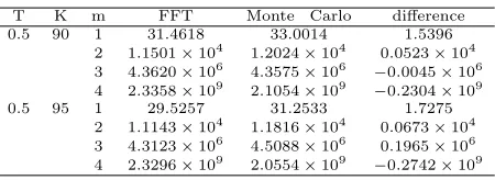
5. Numerical results
In this section, we present and compare numerical results for power call option using the FFT method and the Monte Carlo simulation.
For our FFT method, we take N = 212, a = 600 and α = 0.75. The parameters
are considered as follows r = 0.05, q = 0.06, k1 = 0.9, θ1 = 0.1, σv1 = 0.1, ρ1 =
−0.5, v0(1) = 0.6, k2= 1.2, θ2 = 0.15, σv2 = 0.2, ρ2 =−0.5, v
(2)
0 = 0.7, λJ = 0.22, µs=
0.22, σs = 0.25, ρJ = −0.4, µv = 0.05, S0 = 100 where m, k, T are different. The
numerical results are shown in Table 1. In addition, we takeN= 100,000 simulations
Table 1. Power call option prices: FFT, Monte Carlo.
T K m FFT Monte Carlo difference
0.5 90 1 31.4618 33.0014 1.5396
2 1.1501×10⁴ 1.2024×10⁴ 0.0523×10⁴
3 4.3620×10⁶ 4.3575×10⁶ −0.0045×10⁶
4 2.3358×10⁹ 2.1054×10⁹ −0.2304×10⁹
0.5 95 1 29.5257 31.2533 1.7275
2 1.1143×10⁴ 1.1816×10⁴ 0.0673×10⁴ 3 4.3123×10⁶ 4.5088×10⁶ 0.1965×10⁶ 4 2.3296×10⁹ 2.0554×10⁹ −0.2742×10⁹
to price the power call option using the Monte Carlo simulation.
So numerical results proved that FFT approach is correct and more efficient than Monte Carlo simulation.
6. Conclusion
In this paper we drived the characteristic function and got the power option pricing by FFT. In the sequel, the efficiency of our analytic method by Monte Carlo simulation and numerical results is shown.
Acknowledgment
References
[1] P. Carr and D. Madan,Option valuation using the fast Fourier transform, Journal of compu-tational finance,2(4) (1999), 61-73.
[2] P. Christoffersen, S. Heston, and K. Jacobs,The shape and term structure of the index option smirk: Why multifactor stochastic volatility models work so well, Management Science,55(12) (2009), 1914-1932.
[3] D. Duffie, J. Pan and K. Singleton,Transform analysis and asset pricing for affine jump diffu-sions, Econometrica,68(6) (2000), 1343-1376.
[4] J. Gatheral,The volatility surface: a practitioner’s guide, Vol. 357, John Wiley and Sons, 2011. [5] R. C.Heynen and H. M. Kat,Pricing and hedging power options, Financial Engineering and the
Japanese Markets,3(3) (1996), 253-261.
[6] J. Hull and A. White,The pricing of options on assets with stochastic volatilities, The journal of finance,42(2) (1987), 281-300.
[7] J. Kim, B. Kim, K. S.Moon, and I. S.Wee,Valuation of power options under Heston’s stochastic volatility model, Journal of Economic Dynamics and Control,36(11) (2012), 1796-1813. [8] E. M. Stein and J. C. Stein, Stock price distributions with stochastic volatility: an analytic
approach, Review of financial Studies,4(4) (1991), 727-752.
[9] X. Su, W. Wang, and K. S. Hwang,Risk-minimizing option pricing under a Markov-modulated jump-diffusion model with stochastic volatility, Statistics and Probability Letters,82(10) (2012), 1777-1785.