Available Online at www.ijpret.com 863
INTERNATIONAL JOURNAL OF PURE AND
APPLIED RESEARCH IN ENGINEERING AND
TECHNOLOGY
A PATH FOR HORIZING YOUR INNOVATIVE WORK
FACE RECOGNITION: A HYBRID APPROACH USING EIGENFACES AND
KEYPOINT DESCRIPTOR
SHWETA MITTAL, DEBASISH PRADHAN
Department of Applied Mathematics Defence Institute of Advance Technology Pune, India Accepted Date: 05/03/2015; Published Date: 01/05/2015
\
Abstract: Face recognition is a complex task and there is no such technique which provides 100% recognition rate to all situations and applications in which face recognition may appear. In this paper, the authors propose a new hybrid approach based on Principal Component Analysis (PCA) and Scale Invariant Feature Transform (SIFT) for face recognition. Recognition problem can be viewed as recognizing a test sample in a given database called training set. The basic idea of our method contains three steps. In first step find the eigenfaces of the test image as well as of the images in whole training set by using PCA to get reduced size of training set, which contains the most similar images to the test image. This step is done in order to get a reduced size of the training set. In the second step we apply SIFT method to get the keypoint descriptor for the test image as well as for all the images which are obtained from the first step. Third step involves the matching of keypoint descriptor by using Cosine Angle Distance (CAD).
Keywords: Face recognition, Eigenfaces, PCA, SIFT, Keypoint Descriptor.
Corresponding Author: MS. SHWETA MITTAL
Access Online On:
www.ijpret.com
How to Cite This Article:
Available Online at www.ijpret.com 864 INTRODUCTION
Face recognition problem defined as "Having a database of images called training set and a single test image, and we have to identify the identity of test image in the training set". Face recognition practices have acquired great potential in a wide range of applications in varied domains in the past several decades. The face recognition task has a number of challenges with respect to the change in illumination, pose, scale, facial expression.
There are several methods for face recognition these methods can be classified into three categories [1]. First is feature based approach. In this category, the point or area of interest is extracted from the images and use for the recognition task. Second is Holistic based, in this category the whole image pixel intensity is used for the recognition task. Third category includes the methods that use the combination of both feature based and holistic based methods. PCA is an example of the holistic based approach which is proposed by Karl Pearson and used for face recognition by Tunk and Pentland [2] and subsequently it was discussed by K. Kim [3]. PCA uses the global information for the purpose of the face recognition task. Ben Nui develops a new method Laplacianfaces [4] for the face recognition which is based on Locality Preserving Projection (LPP) [5]. It is a non linear approach which obtains a face subspace that best detects the essential manifold structure of the face. However, this method is invariant to the change in illumination and also robust to outliers but it suffers from change in pose, scaling. SIFT is a feature based approach and one of the latest method for the purpose of face recognition. David G. Lowe proposed a method for the local feature extraction [6] and further extended his work [7]. L. Zhang et al. gives a face recognition method using Recognition Using SIFT and Support Vector Machine [8]. Yu-Yao Wang et al. revised SIFT method and combine it to the Euclidean distance method [9]. To make use of the advantages of both PCA and SIFT some attempts are made in this direction. Yan Ke, Rahul Sukthankar proposed a method [10] for face recognition, which examines local image descriptor by using
SIFT and then apply the PCA.
Available Online at www.ijpret.com 865 PCA
PCA deals with the covariance matrix of a set of variables and it project data from the higher dimensional space to the lower dimensional space by identifying the direction of motion of the data, known as principal direction. It does well only in the linear domain.
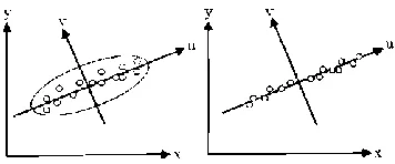
Fig. 1. (a) PCA for data representation (b) PCA for Dimension reduction
Fig.1.(a) and Fig.1.(b) shows the details of PCA for data representation and dimension reduction, respectively [12]. Here, the data are represented in the spatial coordinate system (x-y). In Fig.1, the data move along u and v direction so, u and v are called principal directions or principal components.
Since the motion of data is along u direction is more than that of along the v direction so we can represent the data along u direction only, this can be done by calculating the mean of all data along the v direction and subtract it from all data points to get a single principal component u.
Eigenfaces
PCA constructs a large one dimensional vector of pixels from the two dimensional image and project them onto eigenspace. Eigenspace is calculated by finding the eigenvectors of covariance matrix of all data sets and these eigenvectors are known as eigenfaces or eigenimages.
Algorithm of PCA
Input: Database of M images of size m*n, called training set and one test image which we have to search in the database.
Available Online at www.ijpret.com 866 Step1: Load images
Convert each images into column vector and load them into a matrix of size N*M, where N is the total number of pixels (mxn) in each image and M is the total number of images in database. Let pj represents the pixel values
Xi= [ P1,P2,--PN ]T ; 7=1,2,3,4,....M (1) Step2: Feature Extraction 2.1 Calculate the Covariance matrix. 2.1.1 Calculate the mean of the input faces.
1 M
2.1.2 Subtract the Eq (2) from the each input
images, we arrive at
wt = xt - m (3)
Where, wt is defined as mean centered image. We wish to find M orthogonal vectors e7 corresponding to M eigenvalues k7. We define W is a matrix whose column is composed of column vector wL.
1.1.3 Covariance matrix C is defined as
C= WWT (4)
2.2 Determine the eigenvalues and eigenvectors of the covariance matrix, here "kt and e7 are the eigenvalues and eigenvectors of the covariance matrix C, respectively.
2.3 In decreasing order, we have arranged the eigenvalues as well as corresponding eigenvectors.
2.4 Retain only the eigenvectors with the largest eigenvalues
2.5 Find Feature Vector
Vt = etTwt (5)
Step3: Matching
3.1 Calculate the similarity of the input test image to the each training image based on Euclidean distance.
Available Online at www.ijpret.com 867 3.3 Display the result.
Step4: Display the eigenvectors (Optional). Here, size of W is NxM so that the size of C is NxN which is very large thus it is
computationally complex to find the eigenvalue and eigenvector of C. Note that number of pixels in an image is much greater than the number of images in the database i.e. N>>M. We can write
WTWcol = y/t C0i (6)
Where, col and //1 are the eigenvectors and eigenvalues of WW, respectively. Now multiplying by W to the left on both the sides of the Eq (6), we arrive at
WWTWct)i = Wy/i C0i (7)
Since y/l is constant so Wy/i can be written as / iW. Therefore,
WWT Wcoi = y/iWa>i (8)
WWT (Wa>i) = y/i(Wa>i ) (9)
From Eq (9), we conclude that y/i is the eigenvalue and Wcoi is the eigenvector of WWT. Here the size of WWT is M*M which is very less than NxN. Thus it is computationally easy to compute the eigenvalues and eigenvector of WTW than WW. In step 2.4 we retain only the eigenvctors corresponding to the higher eigenvalues because the eigenvctors corresponding to the higher eigenvalues shows greater variation.
Merits and Limitations of PCA
PCA does not destroy any information in the image, and also it is computationally inexpensive. However, it does well only in linear domain and also retain unwanted variation due to the change in lightening, facial expression, scale, pose. It uses the global information.
SIFT
Available Online at www.ijpret.com 868 Keypoint Descriptor
Keypoint descriptor is a technique to find the point of interest from a gray image. These points are invariant to the variation in scaling, translation and rotation.
Algorithm of SIFT
Input: Database of M images of size m*n, called training set and one test image which we have to search in the database.
Output: One-one mapping. Give an output image from the database which is most similar to the test image.
Step1: Construct the DOG (Difference of
Gaussian) scale Space:
We find the keypoints that are invariant to the scaling, rotation and translation, for this we project the image into scale space. This can be done by performing convolution of image with the Gaussian filter with two different scales and then subtract both the result in order to get DOG. Let I (xy) be the image intensity and G (x,y,o) is a Gaussian filter then DOG is defined as
D(x, y, a) = (G(x, y, ka) - G(x, y, a)) x I(x, y) (10)
Where, G(x, y,a) = _L_e=^ (11)
Let L( x, y,a)be defined as
L( x, y, o-) = G(x, y, ax) xI (x, y) (12)
So we can rewrite Eq (10) by using Eq (12) as
D( x, y, a) = L( x, y, ka) - L( x, y, a) (13)
Gaussian filter is used for blurring of image, hence this step makes the recognition method invariant to the scale and orientation.
Step2: Calculate Keypoints location
Available Online at www.ijpret.com 869 scale and nine neighbors of scale up and down. We consider only the extreme value because they show the higher changes.
Step3: Calculate magnitude of gradient and orientation of each sample points and assign them.This step is done in order to make our method rotationally invariant.
3.1 Assignment of gradient magnitude to each sample points, which is calculated by
m(x, y) = ^( L (x +1, y)-L (x-1, y ))2 + ( L (x, y + 1)-L (x, y-iff (14)
3.2 Assignment of orientation to each sample points, which is calculated by
6(x,y) = tan-1 (x,y +1)-L(x,y-1)/L(x +1,y)-L(x-1,y)] (15)
Step4: Find the keypoint descriptor
This step makes the recognition method invariant to the change in illumination. After that we get the keypoint descriptor that is invariant to scale, rotation, translation and change in illumination.
4.1 Consider 5x5 region around the keypoints and build an orientation histogram having 36 bins for the image gradient around each keypoints.
4.2 Detect the highest peak in the histogram and this value is assigned as orientation to the keypoints.
4.3 The 16x16 region around the each keypoint is considered and it is divided into sixteen 4x4 subregions. Then an orientation histogram having 8 bins is built for each subregion. This will result in 128 elements for each keypoints.
Merits and Limitations of SIFT
Available Online at www.ijpret.com 870 DETAILS OF OUR APPROACH
Let X denotes the test image and Y denotes the set training images. In this paper, the authors find that whether X exist in training set Y or not, if X exist in the training set Y then we find the identity of X in Y. To do this we apply following steps:
Stepl: First apply the PCA on test image and all the images in the training set and retain only top p most similar images. Similarity is checked on the basis of euclidean distance, i.e. difference || ftraining_img - ftest_img || (16)
Here ftrainingjmg is the feature vector of training images and ftest_img is the feature vector of the test image. We find this difference for each of the images in the training set. Image with minimum difference have maximum similarity. The value of p i.e. the number of images passes to the next step will depend upon the size of training set and our requirements.
Step2: Apply the SIFT on the test image and on the p images that are results from the first step.
Step3: Matching by using Cosine Angle
Distance (CAD)
Matching is done to determine the distance between the keypoint descriptors of two different images. In this paper, the authors use cosine angle distance method [13].
d (x,y)= cos-1(x.y) (17)
Here, x.y represents the dot product of two vectors and d (x,y) represents the cosine angle distance between the two vectors. In order to reject the matches that are too ambiguous we use a threshold value r, and a matched is accepted only if its cosine angle distance is less than r times of the cosine angle distance to the second closest match.
EXPERIMENTS AND RESULT
Fig.2. A sample set of 6 images i.e. M=6.
Available Online at www.ijpret.com 871 then we apply PCA to the images in sample set and a test image which can be from the same sample set or from another set. We first apply PCA in order to reduce the data size, then applies SIFT to the reduced data set. For the SIFT method in our experiment we use <r=1.6 and k=V2. For matching by using cosine angle distance we use r = 0.6. We apply our method on six sample images from Extended Yale Face Database B and recognize the known test image with same or different pose and illumination condition.
Fig.5. Apply SIFT on the reduced data set.
Fig.6. Result of our algorithm for a known test image.
Fig.7. Known test image with different pose and illumination condition.
Fig.9. Reduced training set after applying PCA. Fig.3. A known test image from the same sample.
Available Online at www.ijpret.com 872
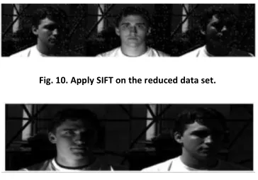
Fig. 10. Apply SIFT on the reduced data set.
Fig. 11. The result of our algorithm for a known test image with different illumination condition and pose.
The authors use the 6 sample images from the Extended Yale Face Database B in Fig.2. And a single known test image taken in Fig.3. Then we apply our method for the recognition of test image in the sample images. First apply PCA and retain only
3(i.e. p=3) images as a reduced set, see in Fig.4. Then we apply SIFT to get keypoints, see in Fig.5. And keypoint descriptor. Finally, we perform matching of SIFT keypoint descriptor of test images and all the images in the reduced sample set. It is done by using the cosine angle distance method. We get a sample image in Fig.6. From the reduced sample set which is same as the test image. We perform the same steps for a known test image in Fig.7. With different pose and illumination conditions and we get an image from the sample set that is most similar to the test image.
CONCLUSION
Face recognition methods have many challenges like change in illumination, pose, scale, rotation that causes major changes the image. The changes that are arising from the change in facial identity with same conditions are less than that of the changes arising in same face identity with the different conditions. So it is very difficult to have 100% accurate method. In this paper, the authors propose a new hybrid approach that combines the advantages of both holistic based approach and feature based approach. This approach also focuses on both global features and local features of the image and also it is computationally less expensive than the others. The authors use a method which is invariant to the change in pose, rotation, scale, illumination conditions.
REFERENCES
Available Online at www.ijpret.com 873 2. M.A. Turk and A.P. Pentland. "Face recognition using eigenfaces," In Computer Vision and Pattern Recognition, 1991. Proceedings CVPR'91., IEEE Computer Society Conference on, pp. 586-591, June 1991.
3. K. Kim, "Face recognition using principle component analysis," In International Conference on Computer Vision and Pattern Recognition, pp. 586¬591. 1996.
4. X. He, S. Yan, Y. Hu, P. Niyogi and H.J. Zhang, "Face Recognition Using Laplacianfaces," IEEE Transaction On Pattern Analysis and Machine Intelligence, vol. 27, pp. 328-340, 2005.
5. Xiaofei He and Partha Niyogi, "Locality Preserving Projection," Neural Information Processing System, pp. 153¬161, 2004.
6. D.G. Lowe, "Object Recognition from Local Scale-Invariant Features," Proceedings of the Seventh IEEE International Conference Computer Vision, vol. 2, pp. 1150-1157, 1999.
7. D.G. Lowe, "Distinctive Image Feature From Scale-Invariant Keypoints," International Journal Of Computer Vision, vol. 60, no. 2, pp. 91-110, November 2004.
8. L. Zhang, J. Chen, Y. Lu, and P. Wang, "Face Recognition Using Scale Invariant Feature Transform and Support Vector Machine," 9th International Conference Young Computer Scientists, pp. 1766¬1770, November. 2008.
9. Yu-Yao Wang, Zheng-Ming Li, Long Wang and Min Wang, "A Scale Invariant Feature Transform Based Mathod," Journal Of Information Hiding and Multimedia Signal Processing, vol. 4, pp. 73-89, April 2013.
10.Ke Yan and Rahul Sukthankar, "PCA- SIFT: A More Distinctive Representation for Local Image Descriptors," In Computer Vision and Pattern Recognition, 2004. CVPR 2004.
11.Proceedings of the 2004 IEEE Computer Society Conference on, vol. 2, pp. II-506, July 2004.
12.A.S. Georghiades, P.N. Belhumeur and D.J. Kriegman, "Illumination Cone Models for Face Recognition under Variable Lighting and Pose," IEEE Trans. Pattern Anal. Mach. Intelligence, vol. 23, no. 6, pp. 643-660, 2001.
13.DOC 493: Intelligent Data Analysis and Probabilistic Inference Lecture 15.