various forms of learning in a
probabilis-tic setting
Bal´azs Gyenis
Institute of Philosophy, HAS RCH 30 Orszaghaz str, Budapest, Hungary
[email protected] fhps.elte.hu/∼gyepi December 26, 2014
Abstract
Jeffrey conditioning is said to provide a more general method of assimilating uncertain
evidence than Bayesian conditioning. We show that Jeffrey learning is merely a particular type
of Bayesian learning if we accept either of the following two observations:
– Learning comprises both probability kinematics and proposition kinematics.
– What can be updated is not the same as what can do the updating; the set of the latter
is richer than the set of the former.
We address the problem of commutativity and isolate commutativity from invariance upon
conditioning on conjunctions. We also present a disjunctive model of Bayesian learning which
suggests that Jeffrey conditioning is better understood as providing a method for incorporating
unspecified but certainevidence rather than providing a method for incorporatingspecific but uncertain evidence. The results also generalize over many other subjective probability update rules, such as those proposed byField(1978) andGallow (2014).
Keywords: Bayesian learning, Jeffrey conditioning, Gallow conditioning, commutativity, formal
epistemology.
1
Introduction
Jeffrey conditioning is a way of obtaining a new probability P2 from an old probability P1 and
P2(H) =P1(H|E), (2)
according to which the new probability P2 is obtained from P1 by (Bayesian) conditioning upon
an evidence E whose prior probability is non-zero P1(E)>0.
On the basis that the Jeffrey formula subsumes the Bayes formula as a special case while it also
seems to allow for conditioning upon non-certain evidence it is frequently asserted in the literature
that Jeffrey conditioning provides a “more general method of assimilating uncertain evidence”
than Bayesian conditioning (Jeffrey; 1983, p. 171). Since the inference ostensibly proceeds from
a contrast between mathematical formulas to a contrast between accounts of learning it clearly
hinges on assumptions about how the mathematical formulas get incorporated into the respective
accounts of learning. We argue that, contrary to the intended conclusion, Jeffrey learning, as well
as many other models of learning (including that of Adams,Field (1978),Gallow(2014) etc.), can
be properly understood as a particular type of Bayesian learning, and Bayesian conditioning is able
to accommodate all these subjective belief revision schemes.
In its most basic form the mathematical structure Bayesianism uses to capture the evidential
reasoning of agents is a probability space. A probability space has two components: a space of
propositions L and a probability measureP defined onL. Correspondingly there are two ways in
which learning can be mathematically modeled in this basic framework:
(i) Probability kinematicstells us how assignments of probability can change.
(ii) Proposition kinematicstells us how the space of propositions can change.
To get a Bayesian account of learning one needs to specify how probability kinematics and
propo-sition kinematics works. The Bayes and the Jeffrey formulas address probability kinematics by
keeping the space of propositions L fixed. Neither of these formulas address proposition
kinemat-ics. In particular, they do not address the possibility of refining the space of propositions. Refining
interpreted as the agent learning new distinctions which she was not able to express before.
Ex-amples include the introduction of new terms to the language: probabilities of propositions which
do not make use of the newly introduced terms remain unchanged, but the agent will now be able
to formulate new propositions as well, on which in turn she may also be able to condition.
Section 2 shows that as long as one does not conflate a single component of Bayesian learning,
namely probability kinematics, with the whole Bayesian account of incorporating evidence, Jeffrey
learning can be properly understood as a particular type of Bayesian learning. Section 3illustrates
the concepts through a simple example and explains why non-commutativity of Jeffrey updates is
not a problem after all.
Section4tackles probability kinematics itself. A mathematical model of updating subjective beliefs
in propositions on the basis of incoming evidence requires two representational elements:
(i) a set of propositions L,
(ii) a set of representations of evidences S on the basis of which the agent may update her
subjective beliefs in propositionsL.
Section 4 argues that by adopting seemingly reasonable assumptions regarding L and S one can
again reach the conclusion that Jeffrey learning can be understood as a particular type of Bayesian
learning, even without taking proposition kinematics into account.
Section 5 takes a detour to show that agents who may be called non-maximal Bayesian face a
paradox of future dependence of conditioning on conjunctions; along the way we isolate two
im-portant desiderata regarding learning models that are often meshed together: commutativity and
invariance upon conditioning on conjunctions. Finally Section 6 proposes a disjunctive model of
Bayesian learning and comments on the irreversibility of Bayesian conditioning. All proofs are
delegated to the Appendix.
2
Probability and proposition kinematics
In what follows P1 and P2 are σ-additive probabilities defined on the same Boolean σ-algebra L
with unit element Ω. It is assumed throughout that the probability P1 is not trivial, i.e. there is
qi≥0, Piqi = 1 such that for all H ∈ L:
P2(H) =
X
i
qi·P1(H|Ei). (4)
As mentioned in the introduction, Jeffrey conditioning without extension is more general than
Bayesian conditioning without extension:
Proposition 2.1 If P2 can be obtained from P1 by Bayesian conditioning without extension, then
P2 can be obtained fromP1 by finite Jeffrey conditioning without extension.
Counterexample 2.1 There is an example where P2 can be obtained from P1 by finite Jeffrey
conditioning without extension but where P2 can not be obtained from P1 by Bayesian conditioning
without extension.
We now also take into consideration proposition kinematics and allow for the possibility of refining
our space of propositions.
Definition 2.3 The probability space ( ˜Ω,L˜,P˜) is an extensionof the probability space (Ω,L, P) if
there exists a probability preserving injective Boolean algebra homomorphism˜fromL to L˜.
Definition 2.4 We say that P2 can be obtained fromP1 by Bayesian conditioning with extension
if there exists an extension ( ˜Ω,L˜,P1˜) of (Ω,L, P1) and an Aˆ ∈ L˜, P1˜( ˆA) > 0 such that for all
H ∈ L:
P2(H) = ˜P1( ˜H|Aˆ). (5)
Definition 2.5 We say that P2 can be obtained from P1 by (finite) Jeffrey conditioning with
ex-tensionif there exists an extension( ˜Ω,L˜,P˜1) of(Ω,L, P1), a partition (with finitely many elements)
{Eˆi}i of Ω˜ withP1˜( ˆEi)>0 andqi≥0, Piqi = 1 such that for all H ∈ L:
P2(H) =
X
i
Proposition 2.2 If P2 can be obtained from P1 by finite Jeffrey conditioning without extension
then P2 can be obtained from P1 by Bayesian conditioning with extension.
Proposition 2.2is a consequence of a slight generalization of Theorem 2.1 of the seminal paper of
Diaconis and Zabell(1982) whose implications would probably have been better appreciated if their
Theorem 2.2 emphasized more clearly the reliance on non-finite partitions (see Counterexample2.3
and Corollary4.2 for further details). The converse of Proposition2.2does not hold:
Counterexample 2.2 There is an example where P2 can be obtained from P1 by Bayesian
con-ditioning with extension, but P2 can not be obtained from P1 by finite Jeffrey conditioning without
extension.
However when extension is allowed on both ends the two notions of conditioning have the same
power:
Proposition 2.3 P2 can be obtained from P1 by finite Jeffrey conditioning with extension if and
only if P2 can be obtained from P1 by Bayesian conditioning with extension.
It is not just mathematically justified to talk about elements of the refined spaces of Proposition2.2
and2.3as ‘propositions’. For instance whenLis generated by taking the smallest Booleanσ-algebra
of a set of propositions of a formal language it is clear from the proofs that an ˜L generated after
the addition of a logically independent proposition can form the basis of the required extension.
Proposition 2.2 shows that an agent can always refine her space of propositions in such a way
that her Jeffrey conditioning corresponds to a Bayesian conditioning upon a proposition ˆA from
the refined space. This includes the elements of the partition: qi = P2(Ei) = ˜P1( ˜Ei|Aˆ) for all
i = 1, ..., n. From this we can see that Bayesian learning can adequately accommodate Jeffrey
learning and there is no need for any new form of ‘input law’ or experience-representing structure
such as the one sought byField(1978). (Field’s proposal have been criticized on other grounds, see
i.e. Garber (1980).) The new information, the “Bayesian factor” can simply come in the form of
a proposition like ˆA and the agent learns how to update her other propositions via basic Bayesian
conditioning upon such ˆA.
Analogues of Proposition2.2can also be obtained for updating rules other than Jeffrey’s, such those
ofField(1978) andGallow(2014). Hence we can also think of these alternative update rules as being
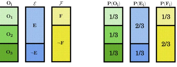
Figure 1: A uniform probability space with three atoms O1, O2, O3 and two element partitions E = {E,¬E} =
{{O1, O2}, O3}, F={F,¬F}={O1,{O2, O3}}.
a proposition from an extended space. Analogues of Proposition2.3 also immediately follow when
the alternative update rule reduces to Bayesian conditioning with a suitable choice of parameters.
See Proposition4.1 and Corollary4.1for details.
The condition that the partition is finite in Proposition 2.2is necessary:
Counterexample 2.3 There is an example where P2 can be obtained from P1 by (non-finite)
Jeffrey conditioning without extension, butP2 can not be obtained fromP1 by Bayesian conditioning
with extension.
The counterexample shows that Jeffrey conditioning can not be obtained in general as Bayesian
conditioning if we allow the partition of propositions whose new probability we set by hand to be
non-finite. Proposition 4.2 and Corollary 4.2 however shows that in a precise approximate sense
Bayesian conditioning is still capable of capturing non-finite Jeffrey conditioning. (It would be
possible but cumbersome to formulate an analogue of Corollary4.2in the framework of this section
and hence omitted.)
3
The problem of commutativity
We illustrate the claims of the previous section with a simple example. Let E be the proposition
that“It is going to rain”andF be the proposition that“RoboCop is going to get wet”, and suppose
that both Alice and Bob initially maintains that the chance of raining is 2/3, the chance of RoboCop
getting wet given that it rains is 1/2, and the chance of RoboCop getting wet given that it does not
rain is 0. As one can quickly check this information can be represented in a uniform probability
With Jeffrey conditioning order-dependence or non-commutativity of successive updates is a well
known concern (see for instance D¨oring (1999)). Suppose that Alice first Jeffrey conditions P to
PE with partition E and corresponding probability valuesqi and then she performs onPE a second
Jeffrey conditioning with partition F and corresponding probability values rj to get PF E. Bob
performs Jeffrey conditionings on the same partitions and probability values, but does so in the
reverse order: first he Jeffrey conditions P to PF with partition F and values rj, and then he
Jeffrey conditionsPF toPEF with partitionE and values qi. It turns out that unlessE andF are
so-called Jeffrey independent with respect toP,qi, andrj (see Theorem 3.2 ofDiaconis and Zabell
(1982)) the result depends on the order in which Alice and Bob updates: PF E 6=PEF.
Thus the order in which Jeffrey conditionings happen does in general matter. On the other hand
it seems reasonable to maintain that the order in which different pieces of evidence arrive should
not matter in the resulting change of subjective beliefs. So non-commutativity is a problem if one
wants to think of the partition and the associated new probability values of the Jeffrey formula as
direct representations of the evidence that is supposed to be incorporated by the agent.
For a concrete example let’s assume that in the first step Alice decreases her belief in the coming
rain (E) to 1/2 and in the second step she increases her belief in RoboCop getting wet (F) to 1/2,
while in the first step Bob increases his belief in RoboCop getting wet to 1/2 and in the second
step he decreases his belief in the coming rain to 1/2. It is easy to check (see Figure 2) that the
corresponding Jeffrey updates do not commute, i.e. PF E(O1) = 1/2 while PEF(O1) = 1/3, and
hence Alice and Bob end up with different beliefs.
According to the intended interpretation Alice first learns that a specific proposition, namely that
it is going to rain, has a chance 1/2. But how does this happen? Alice may look out in the
window and see that the sky is clear; or she may gather this information from the barometer
in her room; or she may hear about it from a radio broadcast. From the mere fact that Alice
alters her beliefs in the coming rain to 1/2 we do not get a definite answer to the question which
among these possible causes prompts Alice to alter her beliefs, nevertheless something does. In the
spirit of Proposition2.2 we can conceive of the actual causal influence on Alice as Alice learning a
proposition (potentially from a refined probability space) with certainty.
Suppose now that we know the actual influences: Alice first decreases her belief in the coming rain
to 1/2 due to seeing that the sky is relatively clear, and second she increases her belief in RoboCop
Figure 2: Illustration of successive Jeffrey conditionings. Alice and Bob Jeffrey conditions on the same partitions
with the same new probability values but in a different order. PE(E) =PEF(E) = 1/2andPF(F) =PF E(F) = 1/2. We see that Jeffrey conditioning is not commutative: PF E 6=PEF, i.e. PF E(O1) = 1/2while PEF(O1) = 1/3.
his beliefs in RoboCop getting wet to 1/2 due to seeing that RoboCop’s umbrella has holes, and
second he decreases his belief in the coming rain to 1/2 due to seeing that the sky is relatively clear.
How it is possible that they arrive to different beliefs, even though they saw “the same things”?
We argue that the intuition expressed by Osherson (2002) for why these Jeffrey updates do not
(and should not be expected to) commute can be made precise and generalized: Alice and Bob
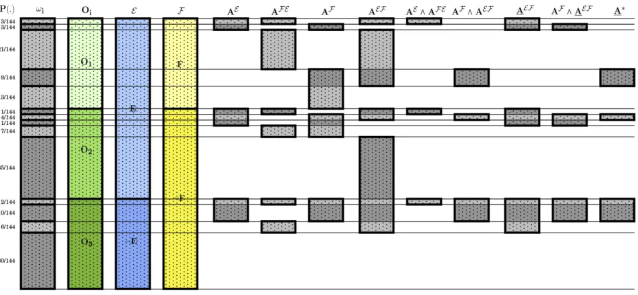
could not have seen the same sky and the same umbrella holes. To illustrate consider an extension
our probability space with 14 atoms; for simplicity we omit the tildes from above the extended
probabilities. With
{ω1, ω2, ω3, ω4, ω5} corresponding toO1,
{ω6, ω7, ω8, ω9, ω10}corresponding toO2,
{ω11, ω12, ω13, ω14} corresponding toO3,
and their probabilities given by Figure 3, the smallest probability space containing {ωi}14i=1 is an
extension of our original probability space.
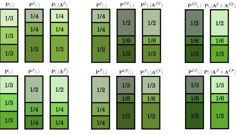
As one can easily verify (see Figure 3 and Figure 4 for details) we can obtain the PE, PF E, PF,
Figure 3: The extended probability space with definitions of various elements.
extension. In other words there exist AE, AF E, AF, AEF in our extended probability space such
that for all H in the original probability space we have1
PE(H) = PAE(H) (7)
PF E(H) = PAEF E(H) (8)
PF(H) = PAF(H) (9)
PEF(H) = PAFEF(H). (10)
ThusAE is a possible representation of the evidence that Alice learns with certainty in the first step
and AF E is a possible representation of the evidence that Alice learns with certainty in the second
step. Similarly AF is a possible representation of the evidence that Bob learns with certainty in
the first step and AEF is a possible representation of the evidence that Bob learns with certainty
in the second step.
The example also shows why the Jeffrey updates fail to commute: the Bayesian factors that induce
the change of subjective beliefs are not the same when the update happens in different order, that
is AE 6= AEF and AF 6= AF E . (And as one could also check, PAE 6= PAEF and PAF 6= PAF E
neither.) Thus if both Alice and Bob revised their beliefs in the chance of rain by consulting the
1
Figure 4: Various probabilities ofO1, O2, O3 assuming that the learning rules are maximal Bayesian.
cloudiness of the sky they could not have seen the same clouds; i.e. the sky Alice saw must have
had more clouds than the one Bob saw. This is also indicated by the fact that Bob performed a
larger revision of belief in the chance of rain (from 3/4 to 1/2) on the basis of his experience than
Alice performed (from 2/3 to 1/2) on the basis of hers.
This non-identifiability of the Bayesian factors that induce non-commutative Jeffrey conditionings
does not hinge crucially upon the specific extension and upon the specific propositions in the
extension we considered. Note first that successively Bayesian conditioning on factors with which
we obtained their respective Jeffrey conditionings do commute as expected: for allHin the original
probability space
PF E(H) =PAE(H|AF E) =PAF E(H|AE), (11)
PEF(H) =PAF(H|AEF) =PAEF(H|AF). (12)
More importantly by conditioning on the conjunction of these Bayesian factors we also obtain the
result of the successive Jeffrey conditioning in our example: for all H in the original probability
space
PF E(H) = PAE∧AF E(H) (13)
IfAE equalledAEF andAF equalledAF E then property (13)-(14) would entailPF E(H) =PEF(H)
for all H in the original probability space, contradicting non-commutativity.
Along the same lines, when we haveanyexample of finite Jeffrey conditionings that do not commute,
and when we haveanyextension withanyBayesian factors satisfying (7)-(10) that have the property
(13)-(14), these Bayesian factors can not be pairwise identified. Thus Alice and Bob could not have
experienced the same pairs of things, no matter what their experience was.
This result also naturally generalizes to the update rules of Field, Gallow etc. Section5is going to
shed light on the perplexing entr´e property (13)-(14) made in this discussion.
4
The updating and the updated
One who has reservations about embracing both aspects of probabilistic learning (probability
kine-matics and proposition kinekine-matics) may consider the following reformulation of the results more
illuminating.
As we mentioned in the introduction we can conceptually distinguish between
(i) a set of propositions L, and
(ii) a set of representations of evidences S on the basis of which the agent may update her
subjective beliefs in propositionsL.
The basic Bayesian approach equates these two elements: L=S. This representational choice is,
however, rather restrictive. Learning the truth of a proposition may clearly count as evidence for
updating subjective beliefs in other propositions; however not all evidence on the basis of which
subjective beliefs in propositions can be updated need to come in the form of a proposition. In
other words, it seems reasonable to assume thatL forms a part ofS, however there are reasons to
assume that S also contains many more elements that are lying outside of L. (Cf. the discussion
in Chapter 11.2 ofJeffrey(1983).)
One can interpret S in different ways. S could be entailed by a detailed physical-psychological
theory of the agent and her possible interactions with her environment. Alternatively,S could also
represent the set of physically possible worlds. Either way it is reasonable to assume thatSis much
richer than the set of propositions of a language that the agent is able to formulate.
Definition 4.1 Let us call a triple(L,S, P)alearning frameif there exists aP¯ probability measure
¯
P( ¯H) etc.
Definition 4.2 A learning frame (L,S, P) is
– basic ifL=S.
– regular if
• P isnon-atomic onS: for any A∈ S withP(A)6= 0there exists a B∈ S, B⊆A,
P(B)6= 0 such that P(B)< P(A).
• P is atomic on L: for any A ∈ L with P(A) 6= 0 there exists a B ∈ L, B ⊆ A,
P(B)6= 0 such that for all C ∈ L, C (B: P(C) = 0.
Example of a regular learning frame: let Ω contain countably many sentences of a language, let L
be the smallest Boolean σ-algebra containing elements of Ω, and let ¯P be a probability measure
on L. There always exists an extension (S, P) of (L,P¯) such that P is non-atomic on S. Then
(L,S, P) is a regular learning frame. Also, whenever (L,S, P) is a regular learning frame and
P(A)6= 0 for anA∈ S then (L,S, PA) is also a regular learning frame.
Definition 4.3 A learning rule is a mapping between learning frames.
A learning rule (L,S, P1)7→(L,S, P2) is
– Bayesian if there exists an A∈ S such that for all H ∈ L:
P2(H) =P1(H|A).
– (finite) Jeffrey if there exists a (finite) partition {Ei}i, Ei ∈ S, P1(Ei) > 0 and qi ≥ 0,
P
iqi = 1 such that for all H ∈ L:
P2(H) =
X
i
– (finite) Gallow 1if there exists a (finite) partition{Ti}i, Ti∈ S,P1(Ti)>0, Ei∈ S,P1(TiEi)>0such
that for allH∈ L:
P2(H) =
X
i
P1(H|TiEi)·P(Ti).
– (finite) Gallow 2 if there exists a (finite) partition {Ti}i, Ti ∈ S, P1(Ti) >0, Ei ∈ S, P1(TiEi) > 0,
∆i>0such that for all H∈ L:
P2(H) =
X
i
P1(H|TiEi)·P(Ti)·∆i.
– Fieldif there exists a finite partition{Ei}2n
i=1,Ei∈ S,P1(Ei)>0, and0< qi<1, P2
n
i=1qi= 1such that
for allH∈ L:
P2(H) =
P2n
i=1e
αi·P
1(HEi)
P2n
i=1eαi·P1(Ei)
whereαi= 21n Q2n
j=1
P2(Ei)
P1(Ei)/
P2(Ej)
P1(Ej) for alli= 1, ...,2
n
.
A few more technical concepts relating to learning rules:
Definition 4.4 A learning rule (L,S, P1)7→(L,S, P2) is
– basic if(L,S, P1) is basic.
– regular if (L,S, P1) is regular.
– conservative if supp(P2)⊆supp(P1).
– bounded if there exists a number α ≥1 such that for all H ∈ L:
P2(H)≤α·P1(H). (15)
Every bounded learning rule is clearly conservative, but the converse is not true.
One can show the following:
Proposition 4.1 Every bounded regular learning rule is Bayesian.
Corollary 4.1 A regular learning rule is
• Bayesian if and only if it is finite Jeffrey,
• Bayesian if and only if it is finite Gallow 1,
• Bayesian if and only if it is finite Gallow 2,
Definition 4.5 A learning rule (L,S, P1) 7→ (L,S, P2) is approximate Bayesian if for all i ∈ N there exists a subset Li ⊆ L, P1(WH∈LiH)→0 as i→ ∞, and an Ai∈ S such that
• for all H∈ L\Li:
P2(H) =P1(H|Ai),
• Li+1⊆ Li, Ai+1 ⊆Ai.
Every approximate Bayesian learning rule is Bayesian (as can be seen by setting Li =∅), but the
converse does not hold.
Proposition 4.2 Every conservative regular learning rule is approximate Bayesian.
Corollary 4.2 If a regular learning rule is either
• Jeffrey,
• Gallow 1,
• Gallow 2,
• Field,
then it is approximate Bayesian.
Proposition4.2and Corollary4.2indicates that the limitation of Bayesian conditioning versus
non-finite Jeffrey conditioning stems not from the relative weakness of Bayesian conditioning as a means
of updating probabilities, but from the lack of an appropriate account of Bayesian conditioning on
sets of measure zero. One can think of Definition 4.5 as providing such an account.2
2
Note that in the definition of a Bayesian, Jeffrey (Gallow, Field etc.) learning rules we only required
the probability updates to work in a certain way for all H ∈ L, and we stayed silent about how
these learning rules should update the probability for otherG∈ S \ L. When learning rules follow
the same probability update formulas for allG∈ S \ Las they do for allH∈ L, we may call them
maximal, i.e. maximal Bayesian, maximal Jeffrey, etc.
If (L,S, P) can assumed to be regular Corollary 4.1 suggests the following model of Bayesian
learning: the agent always updates her subjective beliefs in propositions L by conditioning on
an ˆA ∈ S that she learns with certainty. Now, if what indeed triggers the change in the agent’s
subjective beliefs is learning ˆAwith certainty, then it seems reasonable to require the “true” learning
rule to be maximal Bayesian, that is, to require that the agent updates her probabilities of all
elements in S by conditioning on ˆA. From this it follows, however, that the same learning rule
can in general only be Jeffrey, but not maximal Jeffrey (in the non-trivial sense that excludes the
case when the maximal Jeffrey rule is also maximal Bayesian, that is when we Jeffrey condition on
partition with an event with posterior probability one).
5
Are not maximal Bayesian learning rules viable?
Are not maximal Bayesian learning rules viable? For instance, is it reasonable to assume that
an agent’s subjective belief revisions are occasionally best modeled by a (non-trivially) maximal
Jeffrey learning rule?
The argument we gave in Section4against the viability of maximal Jeffrey learning rules – that is,
against learning rules that update all elements ofS via Jeffrey conditioning – is based on accepting
Bayesian conditioning as the “true” background evidence assimilating procedure. One could insist,
however, that maximal Jeffrey learnings do indeed happen. In the rest of this section we show that
regular learning rules that are not maximal Bayesian yield some paradoxical consequences.
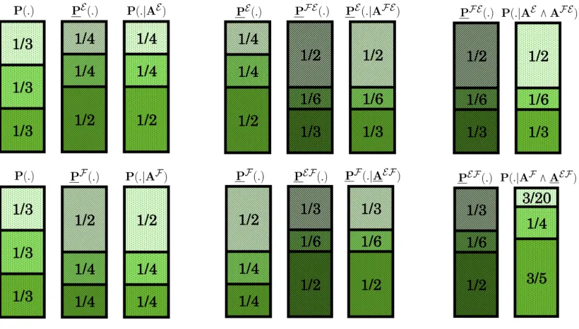
We return to our example from Section3. We consider the same original space, the same extended
space, and same elements in the extended space, but for the updated probabilities we assume that
they are maximal Jeffrey, that is on all elements of the extended space their values are determined
Figure 5: Various probabilities ofO1, O2, O3 assuming that the learning rules are maximal Jeffrey.
by their respective Jeffrey conditioning. We signal this difference by underlining the updated
probabilities.
It turns out (see Figure3and Figure5 for details) that we can obtain thePE,PF E,PF, andPEF
Jeffrey updated probabilities of Alice and Bob from P by Bayesian conditioning with the same
extension. For the same AE, AF E, AF ∈ L, and for a new element AEF we have, for all H in the
original space:
PE(H) = PAE(H) (16)
PF E(H) = PEAF E(H) (17)
PF(H) = PAF(H) (18)
PEF(H) = PFAEF(H). (19)
(We needed to replaceAEF with another element AEF becausePEF(H) does not equalPFAEF(H).)
All seems well. However the example also shows that something strange is going on. We can obtain
PE from P by conditioning on AE, we can obtain PF E from PE by conditioning on AF E, and so
it seems natural to assume that we can obtain PF E from P by conditioning on the conjunction
AE∧AF E. In other words, similarly to the maximal Bayesian case, one could expect that for allH
in the original space:
and similarly
PEF(H) =PAF∧AEF(H) (21)
holds, where i.e. (20) is ostensibly derived as
PF E(H) = PEAF E(H) =PE(H|AF E) =
PE(H∧AF E)
PE(AF E) (22)
= PAE(H∧A F E)
PAE(AF E)
= P(H∧A F E|AE)
P(AF E|AE) =
P(H∧AF E∧AE)
P(AE)
P(AF E∧AE)
P(AE)
(23)
= P(H∧A
F E∧AE)
P(AF E ∧AE) =P(H|A E ∧
AF E) =PAE∧AF E(H) (24)
by using (17) for the first and (16) for the fourth equality. (16) however can not be applied for the
fourth equality as it was only guaranteed by our construction for elements of the original space, of
which AF E is not a member.
As it happens (20) does hold in our example, but its counterpart, (21) does not: i.e. PEF(O1) = 1/3
while PAF∧AEF(O1) = 3/20!3
Thus even though successively Bayesian conditioning on factors with which we can obtain their
respective Jeffrey conditionings do commute as expected, it is not guaranteed that by conditioning
on the conjunction of these Bayesian factors we can obtain the result of successive Jeffrey
condi-tionings when the learning rule is not maximal Bayesian! Commutativity (11) and invariance upon
conditioning on conjunctions (20) are thus separate properties: when the set of things that we can
update are the same as the set of things that can do the updating they both hold, but the latter
does not necessarily follow from the former when these two sets of things do not coincide.
Commu-tativity captures the idea that it shouldn’t matter whether we receive AE first and AF E second or
we receive AF E first and AE second. But it also shouldn’t matter whether we receive AE and AF E
successively or at the same time (meaning that we receive their conjunction AE∧AF E), which is
what invariance upon conditioning on conjunctions expresses. Commutativity and invariance upon
conditioning on conjunctions are often meshed together since they both hold in the basic Bayesian
model, but they express different, albeit equally important desiderata about learning models.
The appearance of failure of invariance upon conditioning on conjunctions can be alleviated to
some degree:
3There does exist anA∗∈ L
– depicted in Figure3– such that for allH in the original space:
PEF(H) =PA∗(H), (25)
Then for all k= 1, ..., N there exists an Ak∈ S such that for all H∈ L:
Pk(H) =Pk−1(H|Ak), (26)
and for which
Pk(H) =P0(H|
k ^
i=1
Ai). (27)
Even thought Proposition 5.1 shows that we can always obtain successive maximal finite Jeffrey
conditionings by successive Bayesian conditionings on factors in a way that by conditioning on the
conjunction of these factors we can also obtain the result of the successive maximal finite Jeffrey
conditionings, there is something deeply disturbing in the construction that is required to achieve
this: in order to determine a Bayesian factor at stagekwe need to have already determined all other
Bayesian factors that will follow after stage k. Thus if we want to reconstruct successive maximal
finite Jeffrey conditionings as Bayesian conditionings with retaining invariance upon conditioning on
conjunctions then we need to require the agent to have foresight in what other Jeffrey conditionings
she will perform in the future. This problem may be labeled as the paradox of future dependence
of conditioning on conjunctions for non-maximal Bayesian learning rules.
The paradox of future dependence of conditioning on conjunctions can only be avoided when the
regular learning rule is maximal Bayesian; in this case invariance upon conditioning on conjunctions
is also automatically satisfied. (In the maximal Bayesian case there is no future dependence since
then condition (33) in the proof of Proposition 5.1is satisfied by all elements of S, not just those
of the form H∧VN
i=k+1Ai, and hence there is no dependence on whatAi,i=k+ 1, ..., N are.)
6
A disjunctive model of Bayesian learning
One may insist that there are cases when the agent only learns new probability values qi on a
partition E and updates her subjective beliefs without learning anything with certainty. Taken
information i.e. on a slip of paper, there have been a change in the interaction of the agent and
the physical world which can be modeled by the agent learning something with certainty, i.e. that
she had the experience of reading this-and-that on a slip of paper. If S is rich enough to represent
such physical interactions and experiences then successive Bayesian conditioning on elements of S
remains an adequate model of updating subjective beliefs.
This is not to say that we shouldn’t want to model situations in which either the proper source
of information – the specific ˆA ∈ S which represents the physical interaction that triggers the
change of beliefs – is uninteresting for the agent, or in which it is impractical or unfeasible or
uninteresting to construct the detailed physical-psychological theory that models the information
interactions of the agent. There are clearly many pragmatic reasons why we may want to rely
on restricted models that do not take these details into account. These pragmatic concerns can
however be accommodated without giving up Bayesian conditioning as the core model of subjective
belief revision. We can easily incorporate into the Bayesian model the lack of specification of the
ˆ
A ∈ S that triggers the change of beliefs by tracking not only the single conditional probability
distribution that is conditioned on ˆA but a set of conditional probability distributions that are
conditioned on elements of S which lead to the same updated probability onL as does ˆA.
This suggests the following disjunctive model of Bayesian learning. Initially the agent’s subjective
beliefs about propositions are represented by a probability space (L,P¯) where ¯P in non-atomic on
L. A detailed physical-psychological theory that models the information interactions of the agent
would assigns to (L,P¯) an extension (S, P) so that (L,S, P) is a regular learning frame; we do not
know the details of how this extension is obtained, but it is sufficient to assume that it exists. The
agent’s subjective beliefs at any later stagenare then going to be represented by a triple (L,S,Pn)
wherePnis a set of probability measures defined onS which all agree with the samePnLprobability
measure defined on L, where P0L = ¯P. Suppose that the agent’s beliefs on L change from PnL to
PnL+1 such that these probabilities satisfy condition (15). (This change of beliefs may be due to,
say, Bayesian, Jeffrey, Gallow, Field etc. sort of conditioning upon a proposition(-partition).) Then
Pn+1 = {P0 :∃Pn∈ Pn,∃A∈ S :∀G∈ S :P0(G) =Pn(G|A)
and∀H∈ L:P0(H) =PnL+1(H)}.
This disjunctive model is based purely on Bayesian conditioning yet is able to accommodate a host of
providing a method for incorporating specificbutuncertain evidence.
Departing from the disjunctive model we close this section with a note on the ostensibly problematic
irreversibilityof Bayesian conditioning. Jeffrey conditioning is often touted as superior to Bayesian
conditioning since it has the advantage of being reversible: mistakes can be erased (Jeffrey; 1983,
p. 172). Indeed an agent should be able to revert a change of belief in a proposition that was
triggered by having a specific experience, for her change of belief in the proposition may also
depend on background assumptions that influence how said specific experience gets evaluated, and
these background assumptions themselves may later change in a way that annuls the effect of said
specific experience. Our account respects this requirement: any mistakes that can be erased on L
by Jeffrey or Gallow conditioning can also be erased by an appropriate Bayesian conditioning on
an element ofS. (Cf. with the criticism Weisberg(2009) mounts against conditionalization on the
basis of not being holistic and with the claim of Gallow(2014) that his proposed update rule does
abide holism.) However sans memory loss we should not expect the agent to be able to erase the
fact that she had the specific experience itself. Thus it is an advantage of our account that both
the facts of committing and erasing a mistake gets recorded in changes of probability on S.
Conditioning on a specific A ∈ L is indeed irreversible in L. However one wonders how serious
this problem is. Typically one wants to think of elements of L as propositions of a language, i.e.
statements of scientific theories. Sans divine intervention no agent is going to learn directly such
scientific statements, but only confirm or disconfirm them via observation and experimentation. If
we accept the ethos that confirmation and disconfirmation of scientific statements via observation
is never absolutely certain, and if we think ofSas containing, among else, the set of representations
of observations via which the agents can confirm and disconfirm propositions inL, then any mistake
that the agent can commit during her quest to confirm or disconfirm statements of scientific theories
Acknowledgement
I’m grateful for substantial discussions I had with M´arton G¨om¨ori, Attila Moln´ar, Tam´as Bitai,
P´eter Juh´asz, G´abor Szab´o, and for helpful comments from attendees of the second workshop of the
Budapest-Krakow Research Group on Probability, Causality, and Determinism, especially those of
Leszek Wro´nski, Zal´an Gyenis, and Sam Fletcher.
Appendix
Proof of Proposition 2.1. IfP2 can be obtained fromP1 by Bayesian conditioning without extension then there
exists anA∈ L,P1(A)>0 such that for allH∈ Lwe haveP2(H) =P1(H|A). IfP1(A) = 1 then choose an arbitrary
E∈ L, 0< P(E)<1 and note thatP2(H) =P1(H|A) =P1(H) =P1(E)·P1(H|E) +P1(¬E)·(H|¬E) and thusP2 is
obtained by finite Jeffrey conditioning fromP1without extension using partition{E,¬E}andq1= 1−q2=P1(E).
IfP1(A)6= 1 thenP2(H) =P1(H|A) = 1·P1(H|A) + 0·P1(H|¬A), which shows thatP2is obtained fromP1by finite
Jeffrey conditioning without extension using partition{A,¬A}and settingq1= 1−q2= 1.
Proof of Counterexample 2.1. LetL={∅, a, b,{a, b}},P1(a) = 1−P1(b) = 0.5,P2(a) = 1−P2(b) = 0.3, then
P2 can be obtained from P1 by finite Jeffrey conditioning without extension by settingE ={a}butP2 can not be
obtained fromP1by Bayesian conditioning without extension, as it can be quickly checked.
The following is a generalization of Theorem 2.1 ofDiaconis and Zabell(1982) that covers probability spaces whose base is not necessarily countable (the proof is essentially the same):
Lemma 1 P2 can be obtained fromP1 by Bayesian conditioning with extension if and only if there exists a number
α≥1such that
P2(H)≤α·P1(H) (28)
for allH∈ L.
Proof of Lemma 1. IfP2 can be obtained from P1 by Bayesian conditioning with extension then there exists an
extension ( ˜Ω,L˜,P˜1) of (Ω,L, P1) and an ˆA∈L˜, ˜P1( ˆA)>0 such that for allH∈ L: P2(H) = ˜P1( ˜H|A). Then for anyˆ
H ∈ L:
P2(H) = ˜P1( ˜H|A)ˆ ≤
1 ˜ P1( ˆA)
·P˜1(H), (29)
which shows that (28) holds withα=P1˜1( ˆA).
On the converse suppose that (28) holds withα≥1. Ifα= 1 then for allH ∈ L: P2(H) =P1(H) and hence the
proposition is obvious with setting ˆA= Ω. Ifα >1 then define P3(H) =
α
α−1P1(H)− 1
α−1P2(H) (30)
for allH∈ L. P3 is a probability on (Ω,L) andP1= α1P2+ (1−1α)P3.
Let ˜L=L×{a, b}. ˜Lis aσ-algebra that contains elements of the form ˆH = (H1, a)∨(H2, b) for someH1, H2∈ L. The
homomorphism ˜ identifies an elementH ∈ Lwith ˜H= (H, a)∨(H, b)∈L˜. Define ˜P1( ˆH) = 1
αP2(H1)+(1−
1
α)P3(H2)
i=1
for allH∈ L, according to Lemma1. Letα= max{2,Pn i=1
P2(Ei)
P1(Ei)}. IfP1(H)>0 thenα≥ Pn
i=1
P2(Ei)
P1(Ei)·P1(Ei|H) = Pn
i=1
P2(Ei)
P1(H) ·P1(H|Ei) and henceα·P1(H)≥
Pn
i=1P2(Ei)·P1(H|Ei) =P2(H). IfP1(H) = 0 thenP2(H) = 0, and
so we can conclude that for allH∈ L: α·P1(H)≥P2(H).
Proof of Counterexample 2.2. Let Ω = {ω1, ω2, ...} be countable, let P1(ωi) = 21i, let ˜Ω = Ω× {a, b} and
˜
ωi= (ωi, a)∨(ωi, b), let ˜P1((ωi, a)) = 21iP1(ωi) = 41i, let ˆA= W
i(ωi, a), and letP2(H) = ˜P1( ˜H|A) for allˆ H∈ L.
Suppose thatP2can be obtained fromP1by (finite or not finite) Jeffrey conditioning without extension with partition
{Ei}i,P1(Ei)>0. It follows that for allωj∈Ω there needs to be an elementEiof this partition such thatωj∈Ei
and
P2(ωj)
P1(ωj)
= P2(Ei) P1(Ei)
(32) (see Theorem 2.2 ofDiaconis and Zabell(1982)). Note thatP2(ωj) = ˜P1((ωj, a)∨(ωj, b)|Wk(ωk, a)) =
˜
P1((ωj,a))
˜
P1(Wk(ωk,a))
=
1
P k41k
· 1
2jP1(ωj) = 3· 21jP1(ωj). Thus P2(ωj)
P1(ωj) = 3·
1
2j, which is different for everyj ∈ N, it follows from (32)
that the{Ei}ipartition contains countably many elements. HenceP2 can not be obtained fromP1 byfiniteJeffrey
conditioning without extension.
Proof of Proposition2.3. Suppose first thatP2 can be obtained fromP1 by Bayesian conditioning with extension,
and thus that there exists an extension ( ˜Ω,L˜,P˜1) of (Ω,L, P1) and an ˆA∈L˜, ˜P1( ˆA)>0 such that for allH ∈ L:
P2(H) = ˜P1( ˜H|A).ˆ
If ˜P1( ˆA) = 1 then choose an arbitrary ˆE∈L˜, 0<P˜1( ˆE)<1 and note thatP2(H) = ˜P1( ˜H|A) = ˜ˆ P1( ˜H) = ˜P1( ˆE)·
˜
P1( ˜H|E) + ˜ˆ P1(¬E)ˆ ·( ˜H|¬E) and thusˆ P2is obtained fromP1 by finite Jeffrey conditioning with extension ( ˜Ω,L˜,P˜1)
using partition{E,ˆ ¬Eˆ}andq1= 1−q2= ˜P1( ˆE). If ˜P1( ˆA)6= 1 thenP2(H) = ˜P1( ˜H|A) = 1ˆ ·P˜1( ˜H|A) + 0ˆ ·P˜1( ˜H|¬A),ˆ
which shows that P2 is obtained from P1 by finite Jeffrey conditioning with extension ( ˜Ω,L˜,P˜1) using partition
{A,ˆ ¬Aˆ}and settingq1= 1−q2= 1.
Suppose second thatP2 can be obtained fromP1 by finite Jeffrey conditioning with extension, and thus that there
exists an extension ( ˜Ω,L˜,P˜1) of (Ω,L, P1), a partition{Eˆi}ni=1 of ˜Ω with ˜P1( ˆEi)>0 and qi≥0,Pni=1qi= 1 such
that for allH ∈ L: P2(H) =Pni=1qi·P˜1( ˜H|Eˆi).For an arbitrary ˆH ∈L˜define ˜P2( ˆH) =Pni=1qi·P˜1( ˆH|Eˆi),and
repeat the proof of Proposition2.2applied to ˜P1 and ˜P2.
Proof of Counterexample 2.3. Let Ω = {ω1, ω2, ...} be countable, let P1(ω1) = 56, P1(ωi) = 31i for i > 1,
P2(ωi) = 21i fori≥1. LetEi=ωi and letP2 be defined by the Jeffrey formula (1).
P(Ek|ωj) = 1 ifk=jandP(Ek|ωj) = 0 otherwise, and thusPiPP2(Ei)
1(Ei)·P1(Ei|ωj) =
P2(Ej)
P1(Ej) = (3/2)
j which goes to
infinity asj→ ∞. Thus there is no constantα≥1 such that condition (28) holds for allωj∈Ω, and henceP2 can
Proof of Proposition 4.1. Assume that a regular learning rule is bounded, that is there exists an α≥ 1 such that for all H ∈ L condition (15) holds. We need to show that there exists anA ∈ S such that for all H ∈ L: P2(H) =P1(H|A).
Whenα= 1 and henceP2(H) =P1(H) the proof is trivial by settingAto be the unit element ofS.
Suppose that (15) holds withα >1. SinceP1 is atomic onLthere exists a set of at most countably many pairwise
disjointOi ∈ L which have the property that P1(Oi) >0 but for allC ∈ L,C ( Oi: P1(C) = 0. Every H ∈ L
can be obtained as H =W
i∈IHOi∨H0 where IH is the set of indexesisuch thatOi⊆H and where forH0 ∈ L:
P1(H0) = 0.
Since due to condition (15) P1(Oi) ≥ α1 ·P2(Oi) for all Oi, and since P1 is non-atomic on S, for all Oi there
exist an Ai ⊆Oi, Ai ∈ S such that P1(Ai) = α1 ·P2(Oi). LetA =WiAi. Then for an arbitraryH ∈ Lwe have
P1(H|A) = P1(W1
iAi)·P1(( W
i∈IHOi∨H0)∧( W
iAi)) = 1/α1 ·P1(Wi∈IHAi) =
1 1/α·
P
i∈IHP1(Ai) =
1/α
1/α·
P
i∈IHP2(Oi) =
P2(Wi∈IHOi) =P2(H).
Proof of Corollary 4.1. The→ directions from Bayesian follows immediately from the fact that with the right choice of parameters finite Jeffrey, finite Gallow 1 and finite Gallow 2 reduces to conditioning (c.f. proof of Proposition 2.1).
To←directions to Bayesian follows from that finite Jeffrey, finite Gallow 1, finite Gallow 2, and Field learning rules are bounded (we showed this for finite Jeffrey in the proof of Proposition2.2, the rest are analogous.)
Proof of Proposition4.2. Let our learning rule (L,S, P1)7→(L,S, P2) be conservative and regular. Since thenP1
is atomic on Lthere exists a set of at most countably many pairwise disjoint Oi∈ Lwhich have the property that
P1(Oi)>0 but for allC∈ L,C(Oi: P1(C) = 0. EveryH∈ Lcan be obtained asH =Wi∈I
HOi∨H0 whereIH is
the set of indexesisuch thatOi⊆H and where forH0∈ L: P1(H0) = 0. LetO={Oi}i.
For every α >1 letOα ={O∈ O:P2(O)≤α·P1(O)},Oα =O\Oα,Lα ={H ∈ L:H = W
O∈OαO}, and let
α=P1(WO∈O
αO) =P1( W
H∈LαH). Since by conservativeness ifP2(O)>0 thenP1(O)>0, for anyO∈ Othere
exists a large enoughα∗so thatO∈ Oα for everyα > α∗, and thus it is clear thatα→0 asα→ ∞.
Let us fix now anα >1. There exists a large enoughβ > αsuch that 1−P2(
W O∈OαO)
β ≤P1(
W
O∈OαO). SinceP1 is
non-atomic onS there exists anAα⊆ W
O∈OαO,Aα∈ S such thatP1(Aα) =
1−P2(WO∈OαO)
β . Also, since for all
O∈ Oα: P1(O)≥α1 ·P2(O) and henceP1(O)≥ 1β·P2(O), for allO∈ Oαthere exist anAO⊆O,AO ∈ Ssuch that
P1(AO) =β1 ·P2(O).
Let Aα = (WO∈OαAO)∨Aα, thenP1(Aα) =P1(( W
O∈OαAO)∨Aα) = P
O∈OαP1(AO) +P1(Aα) = P
O∈Oα
1
β ·
P2(O) +
1−P2(WO∈OαO)
β =
1
β ·P2(
W
O∈OαO) +
1−P2(WO∈OαO)
β =
1
β.
Then for an arbitrary H ∈ L\Lα (H = W
i∈IHOi∨H0 with Oi ∈ Oα fori∈ IH) we have P1(H|Aα) =
1
P1(Aα) ·
P1((Wi∈IHOi∨H0)∧(( W
O∈OαAO)∨Aα)) =
1 1/β·P1(
W
i∈IHAOi) =
1 1/β·
P
i∈IHP1(AOi) =
1/β
1/β ·
P
i∈IHP2(Oi) =
P2(Wi∈IHOi) =P2(H).
Finally note that in the constructionAα and Lα can be chosen such thatAα∗ ⊆Aα and L
α∗ ⊆ Lα whenever
α∗≥α.
Proof of Corollary 4.2. This follows from Proposition4.2and the fact that Jeffrey, Gallow 1, Gallow 2 and Field learning rules are conservative.
?
= P1(H∧ VN
i=3Ai|A2)
P1(VNi=3Ai|A2)
=P1(H∧ VN
i=2Ai)
P1(VNi=2Ai)
?
= P0(H∧ VN
i=2Ai|A1)
P0(VNi=2Ai|A1)
=P0(H∧ VN
i=1Ai)
P0(VNi=1Ai)
=P0(H|
N
^
i=1
Ai).
For this latter it is sufficient to guarantee that
Pk(H∧ N
^
i=k+1
Ai) =Pk−1(H∧
N
^
i=k+1
Ai|Ak) ∀k= 1, ..., N−1, ∀H∈ L. (33)
(33) can be guaranteed as follows: first carry out the construction ofAN that satisfies (26) withk=N by following
the proof of Proposition 4.1. Let thenLN−1 be the smallest σ-algebra containing Land AN. PN−1 is also atomic
onLN−1 and thus we can carry out the construction ofAN−1∈ Sby following the proof of Proposition4.1so that
AN−1 satisfies
PN−1(G) =PN−2(G|AN−1)
for all G∈ LN−1 (instead merely for allG∈ L). Since anyG∈ LN−1 takes one of the three formsG=H∧AN,
G=H∧ ¬AN, orG=H for someH∈ L, this way we guaranteed
PN−1(H∧AN) =PN−2(H∧AN|AN−1)
for allH∈ L.
Let thenLN−2be the smallestσ-algebra containingLN−1andAN−1, repeat the procedure above to obtainAN−2∈ S
that satisfies
PN−2(G) =PN−3(G|AN−2)
for allG∈ LN−2, thereby guaranteeing that
PN−2(H∧AN∧AN−1) =PN−3(H∧AN∧AN−1|AN−2)
for allH∈ Letc. AfterN−1 repetition we obtain the required set ofAN, AN−1, ..., A1∈ S which satisfy condition
(33).
Note that if in the proof of Proposition5.1we alter condition (33) with an appropriately chosenλkto
Pk(H∧ N
^
i=k+1
Ai) =λk·Pk−1(H∧
N
^
i=k+1
Ai|Ak) ∀k= 1, ..., N−1, ∀H∈ L
References
Diaconis, P. and Zabell, S. L. (1982). Updating subjective probability, Journal of the American
Statistical Association77(380): 822–830.
D¨oring, F. (1999). Why bayesian psychology is incomplete?,Philosophy of Science66: S379–S389.
Field, H. (1978). A note on jeffrey conditionalization, Philosophy of Science45(3): 361–367.
Gallow, J. D. (2014). How to learn from theory-dependent evidence; or commutativity and holism:
A solution for conditionalizers,The British Journal for the Philosophy of Science 65: 493–519.
Garber, G. (1980). Field and jeffrey conditionalization,Philosophy of Science47(142–145).
Jeffrey, R. C. (1983). The Logic of Decision, The University of Chicago Press, Chicago.
Osherson, D. (2002). Order dependence and jeffrey conditionalization. Available at http://
philpapers.org/rec/OSHODA.
Weisberg, J. (2009). Commutativity or holism? a dilemma for conditionalizers,The British Journal