R E S E A R C H
Open Access
Single microphone speech separation by
diffusion-based HMM estimation
Yochay R. Yeminy
*, Yosi Keller and Sharon Gannot
Abstract
We present a novel non-iterative and rigorously motivated approach for estimating hidden Markov models (HMMs) and factorial hidden Markov models (FHMMs) of high-dimensional signals. Our approach utilizes the asymptotic properties of a spectral, graph-based approach for dimensionality reduction and manifold learning, namely the diffusion framework. We exemplify our approach by applying it to the problem of single microphone speech separation, where the log-spectra of two unmixed speakers are modeled as HMMs, while their mixture is modeled as an FHMM. We derive two diffusion-based FHMM estimation schemes. One of which is experimentally shown to provide separation results that compare with contemporary speech separation approaches based on HMM. The second scheme allows a reduced computational burden.
Keywords: Single microphone speech separation, Manifold learning, Diffusion maps, Factorial hidden Markov models
1 Introduction
Single-channel speech separation (SCSS) is one of the most challenging tasks in speech processing, where the aim is to unmix two or more concurrently speaking sub-jects, whose audio mixture is acquired by a single micro-phone. The goal is therefore to decompose the single input signal into multiple output channels, each dominated by a single speaker. The core obstacle in such tasks is the lack of spatial information, and the common statistical characteristics of the mixed signals.
Single-channel speech separation was studied by sev-eral schools of thought, where computational auditory scene analysis (CASA) proved to be among the most effective. CASA-based methods are motivated by the abil-ity of the human auditory system to separate acoustic events, even when using a single ear (although binau-ral hearing is advantageous). CASA techniques imitate the human auditory filtering known as cochlear filtering, where time-frequency bins of the speech mixture are clus-tered using psychoacoustic cues such as the pitch period, temporal continuity, onsets and offsets, etc. The cluster-ing associates each time-frequency bin with a particu-lar source. The time-frequency bins associated with the desired source are retained, while those associated with
*Correspondence: [email protected]
Faculty of Engineering, Bar-Ilan University, Building 1103, Ramat-Gan, Israel
the interference are attenuated. Such approaches were studied by Weintraub [1], Parsons [2], and Brown and Cooke [3]. Contemporary CASA schemes utilize oscil-latory correlations [4], and common amplitude modula-tion [5], but do not utilize prior informamodula-tion regarding the source signals and their number. All they require is that each time-frequency bin is dominated by a single speaker. A probabilistic interpretation of CASA was pro-posed by Wang and Brown [6], and applied by Vincent and Plumbley [7], who proposed a Bayesian formulation of the separation based on a harmonic model of the sources.
The association of each time-frequency bin with a par-ticular speaker is usually referred to as binary or hard masking. In the ideal case, where the time-frequency bin association of each source is perfectly known, the mask is usually referred to as the ideal binary mask (IdBM), and it was shown by Li and Wang [8] to be optimal in terms of source to noise ratio (SNR). Yilmaz and Rickard [9] showed that (ideal) binary masking enables the separation of up to ten sources from a single mixture.
Alternatively, asoftmask can be used, where each time-frequency bin is assumed to be associated with multiple signals (with different weights), and their relative spectral content in each time-frequency bin has to be estimated.
Blind source separation (BSS)-based approaches are commonly implemented via independent component
analysis (ICA), and are widely used in multi-microphone speech separation. In the SCSS context they are for-mulated as an undetermined BSS problem [10, 11]. Zibulevsky and Pearlmutter [12] used the Fourier coeffi-cients to represent speech signals and utilize their sparse-ness for separation.
Van der Kouwe et al. [13] conducted an experimental study that compared CASA [4] to multi-microphone BSS approaches (joint approximate diagonalization of eigen-matrices (JADE) [14] and second order blind identifica-tion (SOBI) [15] algorithms), and showed the advantage of the latter approaches that utilize spatial information. However, in many important application, such a spatial information is unavailable.
Recent separation schemes applied non-negative matrix factorization (NMF), where the magnitude of the Fourier transformed frames is factorized as the product of two non-negative matrices. The first comprising the basis functions, and the second encoding the weights of the corresponding basis functions. The matrix of basis func-tions is speaker-adaptive, learned in a training phase. In the separation stage, the power spectral density (PSD) of the mixture is modeled by a linear combination of the basis functions of both speakers. The corresponding weight matrices are estimated, and utilized to estimate the underlying sources. Virtanen [16] proposed an NMF approach that encourages PSD continuity and sparseness. Smaragdis [17] proposed a convolutive form of the NMF to model the time dependencies of the PSD. A semi-supervised real-time NMF algorithm was proposed by Joder et al. [18]. Only one source is learned from training data whereas the other source is estimated based on the recent past of real-time data.
Benaroya et al. [19] express each source as a weighted sum of temporal Gaussian stationary processes, with pos-itive, slowly time-varying weights. The PSD is approx-imated by the weighted sum of the variances of the Gaussian processes, yielding a non-negative representa-tion, and the sources are recovered utilizing the Wiener filter. Blouet and Cohen [20] extended this factoriza-tion [19] to separate speech from speech-music mix-tures, where the weighted sum of processes approximates the short-time Fourier transform (STFT) of each source as complex-Gaussian stationary processes. A sinusoidal modeling of the time-domain was proposed by Mowlaee et al. [21], where a codebook is trained for each source and utilized in the separation stage. This work was extended in [22], and includes a preceding stage of detecting double-talk or single-double-talk frames, as well as a speaker identifica-tion system.
Machine learning approaches were applied to speech separation by Bach and Jordan [23]. They proposed to treat the separation problem in the time-frequency domain as a segmentation problem and to apply
the relevant segmentation tools to the audio features extracted from the speech spectrogram.
Deep learning techniques are gaining popularity fol-lowing their success in single-talker automatic speech recognition tasks. Essentially, the networks are trained based on parallel sets of mixtures and their constituent target sources. They are optimized to predict the source of the target class, usually for each time-frequency bin. For example, in [24], the speakers are estimated by jointly optimizing a soft time-frequency mask layer with deep recurrent neural networks. However, these works often assume speaker-dependent models with few target speak-ers that are known during training. In addition, they usually work on limited vocabulary and grammar. Yu et al. [25] proposed a speaker-independent method for multi-talker speech separation by using permutation invariant training. It first determines the best output-target assign-ment and then optimizes the separation regression error given the assignment. Another speaker-independent tech-nique is proposed in [26], where contrastive embedding vectors are assigned to each time-frequency region of the spectrogram. It results in implicit prediction of the segmentation labels of the target spectrogram from the input mixtures. Separation is obtained by optimizing K-means with respect to the unknown assignment. In [27], the authors propose to use an ensemble of deep neural networks and demonstrate the superiority of this struc-ture over speech separation algorithms based on a single network.
A plethora of approaches utilize statistical models of speech signals. In [28], the PSD of each speech frame is computed by iterating between randomly drawing fre-quency bins from a mixture of multinomial distributions, and scaling the histogram of the drawings. Given the probabilistic models, the minimum mean square error (MMSE) estimate of the desired source is derived. Essen-tially, this method is virtually indistinguishable from methods applying NMF.
Gaussian mixture models (GMMs) and HMMs are ex-tensively utilized in speech separation tasks. Kristjansson et al. [29] modeled the log-spectrum of each speaker by an GMM. They approximate the joint probability density function (p.d.f.) of the log-spectra of the speakers given the log-spectrum of the mixture, by a normal distribution. Using this approximation, the posterior distributions of the log-spectrum of each speaker are computed, and the MMSE estimator is derived. GMM-based representations can be modified to improve the temporal modeling. Such an approach was proposed by Benaroya et al. [30], where the variances in the GMM are scaled by time-varying factors, to incorporate source dynamics.
recognition, and was denoted as MIXMAX. Burshtein and Gannot [32] reformulated MIXMAX, by assuming that the log-spectrum of the clean speech segments can be modeled by GMMs, while the noise log-spectrum is nor-mally distributed. In particular, the log-spectrum of the noisy speech is approximated by the maximum of the log-spectrum of the speech and noise. This result was extended by Yeminy et al. [33], who proposed a general-ized formulation, incorporating the correlation between adjacent frequency bins. Reddy and Raj [34] applied the MIXMAX model to the speech separation task, where both input signals were modeled by GMMs, and derived two estimators. The first optimizes the MMSE, and the second uses a soft mask, computed using the posterior probability of the observed log-spectrum to match the log-spectrum of the desired speech. Radfar and Dansereau [35] used a similar model as in [34] with an additive error model, assuming that the error is zero-mean and normally distributed. The log-spectra of the speakers are recovered by optimizing the MMSE.
Roweis [36] modeled the log-spectra of the two speak-ers as the output of HMM processes. Using the log-max approximation, the log-spectrum of the mixture signal is approximated by the maximum between the correspond-ing outputs of the two underlycorrespond-ing HMMs, and is modeled by an FHMM. The compound state of the log-spectral vector of the mixed signal consists of two states, corre-sponding to the speakers. A variant of the Viterbi algo-rithm, denoted as factorial Viterbialgorithm, is used to reconstruct the log-spectra of the speakers, while a binary mask is applied to recover the source. This approach was extended by Radfar et al. [37], to the case where the mix-ture of the two sources is a weighted sum of the noise-free speech signals. The gain factors are recovered by an iter-ative formulation of the FHMM, resulting in improved experimental results. However, in [37], the complexity of the algorithm is quadratic in the number of states, and the speaker-to-speaker ratio range must be an input of the algorithm. Hu and Wang [38] proposed an iterative separation scheme that estimates the gain factor with-out any prior knowledge. An HMM is trained for each source, where the utterances of the sources are scaled to have a known equal energy. The mixing model is the log-max approximation and the compound states are inferred using factorial Viterbi algorithm. Each loop of the algo-rithm consists of several steps. A separation phase, where the sources are estimated. Then, the speaker-to-speaker ratio is assessed using the estimated sources. Eventually, the pre-trained models of the speakers and the mixture are adapted to the estimated gain factors. It was reported in [38] that best results were obtained when the separation was based on the MAP estimation.
Hershey et al. [39] also proposed to utilize both FHMM and log-max approximation. The FHMM encodes the
grammar dynamics of the sources, when the structure and vocabulary of each unmixed speech are known in advance. At each grammar state, the dynamics of the acoustics of each source is encoded by an GMM which is based on the log-max approximation. The grammar dynamics takes into account temporal long-term compo-nents of the speech, with respect to the acoustic dynamics, yielding improved experimental results, that in some sce-narios even outperform human listeners. Weiss and Ellis [40] proposed a similar model, where the speech char-acteristics are unknown a priori, but adapted iteratively. Ming et al. [41] proposed a data-driven technique that is also based on long-term temporal dynamics, intended for the general scenario in which the vocabulary and grammar are unknown. A combined FHMM and NMF approach was presented by Mysore et al. [42], and denoted non-negative hidden Markov model (N-HMM). For each source, several small spectral dictionaries are learned. Their evolvement in time is also learned via HMM. The composite signal of the two sources is separated by apply-ing a soft mask, generated by an estimation-maximization (EM) procedure that estimates the contribution of each source at each time-frequency bin. Good separation per-formance is reported for this N-HMM technique. A related work is [43], where a new model called facto-rial scaled hidden Markov model (FS-HMM) combines Gaussian scaled mixture model and NMF. The FS-HMM is utilized in [43] for speech separation and polyphonic audio representation.
The high dimensionality of the log-spectral vectors and the large number of states of the factorial model, imposes high computational burden for the FHMM infer-ence. Roweis proposed to mitigate the high computational burden by detecting pairs of states with the highest obser-vation likelihood, and limiting the factorial Viterbi cal-culations to their corresponding paths. In [38], the beam search [44] is used to speed up the inference process. A band quantization approach that reduces the number of HMM states, was proposed by Rennie et al. [45] to reduce the computational complexity.
from the sparseness of the model. Those states can be used to explain the observations, rather than using all of the possible pairs of states. Rennie et al. [46] applied a similar model able to separate up to four speakers using loopy belief propagation and variational inference that reduce the inference complexity. The max-sum algo-rithm, which is also a belief propagation technique, is also employed by [47] to track multiple pitch trajecto-ries described by an FHMM. Reyes-Gomez et al. [48] proposed to group several frequency bins into frequency bands, such that each frequency band is modeled by an HMM.
Dimensionality reduction schemes were also applied to speech separation. Michalevsky et al. [49] applied the dif-fusion framework [50] to speaker identification, where a feature vector consisting of the mel frequency cepstral coefficients (MFCC) and their first temporal derivative is used to parameterize the manifold of each speaker, by embedding them into a lower dimensional space. Samples are classified by a k-nearest neighbors (k-NN) classifier applied to the embedding of the corresponding feature vector.
In this work we propose the following contributions: First, we derive a novel non-iterative speech separation approach based on the diffusion framework [50], to compute HMM and FHMM models. A comprehensive set of experimental results exemplify the applicability of the proposed method. It is shown that the proposed scheme provides separation results that compare with contemporary speech separation approaches.
Second, by analyzing the asymptotics of Markov random walks, we show that the proposed scheme allows to directly estimate the states of the HMMs and FHMMs, without having to assume any underlying observation model, nor to apply
EM-based iterative training. Hence, the estimation of the Markov states and transitions is decoupled from the estimation of the emission p.d.f.s, and their corresponding parametric model. Thus, we propose two FHMM-based approaches that estimate the underlying HMM in the diffusion domain. The first, provides a direct extension of the FHMM, where the underlying HMMs are computed in the diffusion domain, and the Gaussian observation models utilize the log-max approach applied in the original domain. We denote this approach hybrid FHMM (HFHMM), as it utilizes both the temporal and diffusion
domains. In the second approach, denoted dual FHMM (DFHMM), we estimate the emission p.d.f.s in the diffusion domain, without assuming an explicit emission p.d.f. model. The underlying HMMs are computed similarly to the HFHMM approach.
Last, we propose to utilize the diffusion embedding as a nonlinear projection of the input mixture onto the manifolds spanning each of the speakers. Thus, we aim to utilize the diffusion embedding as a manifold-adaptive projection operator, where the states of each speaker are detected by an FHMM in its manifold. The HFHMM is experimentally shown to compare with previous results [36], and is shown to outperform DFHMM. The latter requires low computational cost, and can be applied alongside other approaches [39] in the low-dimensional space to further reduce the computational complexity.
The remainder of this paper is organized as follows. Section 2 formulates the monaural speech separation problem of two equi-power and pre-trained sources. The diffusion framework, the Nyström extension [51] and the HMM inference using the diffusion maps are surveyed in Section 3. The proposed diffusion-domain speech separation schemes are presented in Section 4, where we detail the separation and training procedures, and propose two alternative mask functions. The pro-posed approaches are experimentally verified in Section 5, and their performance is compared with contemporary schemes. The computational complexity of the HFHMM and the DFHMM schemes is discussed in Section 6, while conclusions and future directions are discussed in Section 7.
2 Problem formulation
The speaker separation problem is often formulated as an FHMM problem. Leta[n] andb[n] be the speech signals of the first and second speakers, respectively, wherenis the discrete time index. We assume that the speech signals are of equal power
n
a2[n]=
n
b2[n]=1, (1)
and thata[n] ,b[n] are zero mean and statistically inde-pendent. For the unequal power model, the reader is referred to [37, 38]. The observed signal is a mixture of the two speakers
z[n]=a[n]+b[n] , (2)
and the objective of the separation scheme is to compute the estimates, aˆ[n],bˆ[n] of a[n] andb[n], respectively, givenz[n]. LetA(,k)be the STFT ofa[n], whereis the temporal frame index and 0≤k≤K−1 is the frequency index. Denoteaas theK/2+1 dimensional vector, whose kth element is
ak=log|A(,k)|; k=0, 1,. . .,K/2.
The core assumption of our approach is that a and bare the observed outputs of two separate HMMs, one per speaker, denoted HMMa and HMMb, respectively.
Let Sa be the number of states in HMMa, and sa be
the state of HMMa at time frame . The probabilistic
attributes of HMMa are given by the initial
probabili-ties Prsa1=si,a = πia,i = 1,. . .,Sa, wheresi,a is the ith state of the first speaker. The transition probabilities are given by Prsa =sj,a|sa−1=si,a = paij; the emission p.d.f. is pa|sa =si,a = Na;μai,Qai, i.e., normally distributed with mean vector μai, and a covariance matrixQai.
HMMb is defined mutatis mutandis such that
there are Sb states with Pr
sb1=si,b
= πb
i;
Pr
sb =sj,b|sb−1=si,b
= pbij; and p
b|sb =si,b
=
Nb;μbi,Qbi
, where we assume Sa = Sb in sake of simplicity.
The mixture process can be modeled by the FHMM [36] that comprises two underlying HMMs evolving indepen-dently over time, each corresponding to a single speaker. At each time instant, the observed samplezdepends on the states of HMMaand HMMb, emitting the latent
out-puts{a,b}, respectively, such thatz=ξ (a,b), where
ξ (·,·)is the mixing function.
Roweis [36] used thelog-maxmixing function approxi-mation (see [31, 52])
z≈max(a,b). (3) Nádas computed the probability ofzanalytically. How-ever, in our scenario, as two speech signals are involved, the sparsity of the signals can be utilized
p(z|sa=i,sb =j)=N(z;μij,Q) (4) whereμij = max(μia,μbj)andQis the covariance matrix of the observation, assuming that∀i,jQai =Qbj =Q.
3 The diffusion framework and the Nyström extension
The diffusion framework is the core computational tool used in our work. The fundamentals of the diffusion framework [50] are detailed in Section 3.1, and the Nys-tröm extension is described in Section 3.2. The asymptotic properties of random walks that pave the way for a novel approach for HMM and FHMM estimation, are discussed in Section 3.3. A systematic approach for estimating the HMM parameters based on the diffusion framework is presented in Section 3.4.
3.1 Diffusion maps
The diffusion framework is an advanced approach for dimensionality reduction [53]. Let = {x1,x2,. . .,xL} be a set of L points, such that xi ∈ Rd. is viewed
as the nodes of an undirected graph, where the weight w(xi,xj) of the edge connecting xi and xj is the
affin-ity between the two nodes. The kernel functionw(·,·)is symmetric, nonnegative, and is commonly based on an application-specific distance measure between the points
. For instance, in speech processing, it is common to compute the distance between MFCC features [49], or log-spectrum feature vectors. The radial basis function (RBF) kernel is often used:
w(xi,xj)=exp
−xi−xj2/ε2
=exp
−dij2/ε2
(5)
wheredijxi−xj2. In addition, hereε >0 such that if
xiandxjare similarw(xi,xj)∼1, andw(xi,xj)∼0 if they
are dissimilar, implying that the corresponding affinity graph nodes are disconnected.εis a scale factor quanti-fying the scale of the similarity, asxiandxjhave nonzero
affinity fordij<3ε, approximately.
LetWbe the affinity matrix such thatwij = w(xi,xj),
and a corresponding Markov matrix is computed by
P=F−1W (6)
where F is a matrix such that fii = jwij and the
non-diagonal entries are zeros. pij can be viewed as the
transition probability fromxi to xj in a single time step.
Taking the tth power ofP is equivalent to running the Markov chain forwardttime steps. This Markov chain has a unique stationary distributionφ0such thatφ0TP = φ0T [50]. In the pre-asymptotic regime, the transition proba-bility fromxitoxjcan be expressed using the biorthogonal
spectral decomposition: pt(xi,xj)=
l≥0 λt
lψl(xi)φl(xj), (7)
where 1 = λ0 ≥ |λ1| ≥ |λ2| ≥ . . . are the (right) eigenvalues ofP, and{ψl},{φl}are the corresponding right and left eigenvectors, respectively. Due to the spectrum decay, the termpt(xi,xj)in (7) can be well approximated
by summing only a few elements.
The induced Markov chain is utilized to define the diffusion distance
D2t(xi,xj)=
y∈
(pt(xi,y)−pt(xj,y))2 φ0(y)
. (8)
This metric evaluates the connectivity of the pair of nodes xi,xj through the entire graph, by the weighted
distance between the conditional probabilities pt(xi,·)
andpt(xj,·) induced by the random walk. The diffusion
distance can be computed by the eigenvalues and right-eigenvectors ofP[50]
D2t(xi,xj)=
l≥1 λ2t
l
Due to the spectral decay, the diffusion distance Dt(xi,xj)can be approximated by a relatively low number
of eigenvectors in (9). Hence, the right eigenvectors{ψl} can be used asa new set of coordinatesfor the set, such that the Euclidean distance between these diffusion coor-dinates{ψl}approximates the diffusion distance in (9). Let m(t)be the number of terms retained, then thediffusion map(embedding) is given by
t:xi −→
λt
1ψ1(xi),λt2ψ2(xi),. . .,λtm(t)ψm(t)(xi)
. (10) forxi ∈ . Note thatψl(xi)for 1 ≤ l ≤ m(t)is theith
coordinate ofψl, thelth eigenvector ofP.
3.2 Nyström extension
The Nyström extension [51, 54] is a numerically efficient approach to extend the embedding vectors{ψl}defined on a set= {xi}Li=1to a sample pointx˜∈/. Namely, we aim to computet(x˜). The crux of the Nyström extension is to computet(x˜)without having to recompute the embed-ding ofby forming a(L+1)×(L+1)affinity matrix and its eigenvectors. The Nyström extension is given by
ψl(x˜)=
1
λl L
i=1
p(x,˜ xi)ψl(xi) (11)
for each eigenvectorψl, and p(x,˜ xi)= Lw(x,˜ xi)
j=1w(x,˜ xj)
. (12)
The weighting by 1/λl implies that due to the decaying spectrum of the Markov matrix, the Nyström extension can be applied to a limited number of eigenvectors to ensure numerical stability.
Since our models will be trained on a massive amount of data, the Nyström extension can help reduce the dimen-sions ofPand, thus to reduce the computational burden and to mitigate the storage requirements.
3.3 The asymptotics of random walks and their convergence properties
The diffusion maps scheme utilizes numerically induced random walks to analyze data sets, by forming the diffu-sion kernel and the correspondingdiscreteeigenfunction
{ψl}computed with respect to the discrete domain (set)
= {xi}Li=1. This approach aims to study the intrinsic continuousmanifoldof the data, via its sampled finite manifestation.
Nadler et al. [55] showed that as the number of data points L → ∞the random walk on the discrete graph manifested by the Markov matrixP, as in (6), converges to a random walk on the continuous space, manifested by the Fokker-Planck operator. The convergence is given by the
convergence of the eigenfunctions of the discrete graph to those of the underlying continuous Fokker-Planck operator{ψl}
lim
N→∞ψl=ψl. (13)
In the continuous domain, systems with potential wells are characterized by their eigenfunctions, where the sta-ble states of the underlying Markov process, correspond-ing to the potential wells are points of high density in the metric eigenfunctions space {ψl} . Nadler et al. [56] extended these classical results asymptotically to the dis-crete domain, showing that as the disdis-crete eigenfunction
{ψl}approximate the continuous ones, the points of high density in the discrete domain estimate those of the cor-responding continuous ones.
This implies that a diffusion embedding computed as in Section 3.1 with respect to a finite and discrete set of points can be used to approximate the states of alatent Markov walkgiven its discrete manifestation
. In particular, given that the intrinsic representation of the data and corresponding Markov system is assumed to be low dimensional, implies that it can be represented by a few leading eigenvectors. In speech analysis, the low dimensionality of the system stem from the multiple constraints induced on a human speech process by the physical attributes (the anatomical structure of the mouth, tongue etc.), as well as social conventions.
Lafon and Lee [57] studied the quantization of the cor-responding Markov chain and graph, aiming to derive a computational approach for recovering the stable meta-states and showed that the optimal quantization with respect to the diffusion distance as in (9) is given by the centroids computed by the K-means quantization scheme with an Euclidean distance metric, in the dif-fusion domain. Their result stems from the equivalence between the optimal L2 distances (optimized by the K-means scheme) and the diffusion distances. Hence, given a set ofLpoints, their quantization in the diffusion space allows to optimally approximate the meta-states of the latentMarkov system [57], in terms of diffusion distance distortion.
3.4 Learning an HMM with diffusion maps
estimation of the emission p.d.f.s, and avoids the iterative training of the classical EM-based approach.
Let the set of samples = {x}L=1∈Rdbe a sequence of HMM emissions. The HMM hasSstates with transition probabilities {pij}Si,j=1, initial probabilities {πi}Si=1, mean vectors{μi}Si=1, and covariance matrices{Qi}Si=1.
The diffusion embedding of {x}L=1 is denoted by {¯x}L=1 ∈ RD, where D d. In order to identify the meta-stable states of the random process manifested by
{x}L=1, we quantize the embedding coordinates{¯x}L=1 intoS meta-states, denoted as{si}Si=1, using the K-means algorithm. TheL2distance in the embedding domain cor-responds to the diffusion distance, and allows to coarsen the corresponding Markov chain.
The computed meta-states are utilized to estimate the parameters of the HMM. The transition probabilitiespij
are estimated by running the training samples through the meta-states siSi=1, and accumulating the transitions in a S×Stransition histogram. For that, each sample{¯x}L=1 is associated with its closest meta-state in{si}Si=1, in terms of theL2norm.μiis the average of the high-dimensional
vectors{x}L=1belonging to a statesi. The initial probabil-ities and the covariance matrices are estimated similarly.
An example demonstrating the learning procedure and its results are given in Appendix.
4 Speech separation by diffusion maps
In this section, we introduce two novel speech separa-tion schemes based on the diffusion framework. In both, we derive data-driven speech models for recovering latent state-space models, whereSaandSb, are the first and
sec-ond speakers, respectively, and the FHMM models are trained with respect to them.
4.1 Hybrid-FHMM
We propose to train an HMM model per speaker using the diffusion framework following Section 3.4. Given the speaker’s estimated meta-states and the corresponding probabilities found in the training step, the observa-tion (emission) p.d.f.s are computed in the log-spectral domain, using the log-max formulation in (4). With these emission p.d.f.s, the factorial Viterbi algorithm is car-ried out in the log-spectral domain to infer the states sequences of the speakers, as suggested in [36]. Finally, a masking mechanism is applied to the mixed signal based on the decoded states. We denote this method HFHMM, as it utilizes both the (original) log-spectral domain as well as the (embedded) diffusion domain. The training of the model is carried out in the low-dimensional space, and the inference in the high-dimensional log-spectral domain. By testing the HFHMM (and comparing it to [36]), it will be easy to demonstrate that the new training procedure, at the very least, does not come with performance penalty.
4.1.1 Training phase
Let u[n] be the discrete temporal samples forming the training set ofSa. We start by computing the log-spectral
frames a = {u}M=1 ∈ Rd, where each frame u comprises d = K/2 +1 frequency bins. The diffusion embeddingof{u}M=1is denoted by{¯u}M=1 ∈RD, where Dd. Throughout this paper, over-bar designate term in the embedded space. In order to identify the meta-stable states of the random process manifested by {u}M=1, we quantize the embedding coordinates {¯u}M=1 into Sa = Sb = S meta-states, denoted{si,a}S
i=1, using the K-means algorithm. Although one can set a different value of states to each speaker, the same value was used for both, in sake of simplicity.Sis on the order of tens of states due to the limited number of training data points. The tran-sition probabilitiespaij and the log-spectral mean vectors
{μa
i}Si=1are estimated following section 3.4, and a similar procedure is applied tov[n], the temporal samples ofSb.
The training phase is depicted in Fig. 1, where the HMM of the speakers are trained separately, and their coupling is formulated by the observation probability within the FHMM framework.
4.1.2 Test phase (latent state estimation)
The decoding phase of the proposed HFHMM scheme identifies with that of [36]. Let z[n]= a[n]+b[n] be a test mixture signal, where a[n] and b[n] are the utter-ances fromSa andSb, respectively, and{z}N=1 ∈ Rd its
corresponding log-spectral vectors. The observation p.d.f. is modeled in the spectral domain utilizing the log-max approximation, similarly to (4). The underlying states of the speakers are estimated using the factorial Viterbi algorithm (see Algorithm 1) given the models inferred in the training phase. The separation is implemented by adaptively masking the speakers (see Section 4.3).
4.2 Dual-FHMM
In the second proposed approach, we derive a novel formulation for estimating the emission (observation) p.d.f.s of the speech mixture directly in the diffu-sion domain, as opposed to the HFHMM scheme. The meta-states of the underlying Markov processes (mod-eling the speakers) are estimated by K-means based training in the diffusion domain, as in the previous section.
We propose to synthesize an artificial mixture signal consisting of randomly combined training segments of both speakers. Two FHMM are trained in two differ-ent diffusion domains, one FHMM per speaker. Since each diffusion domain is based on the segments of one particular speaker, it is best adapted to that speaker. Denote these models FHMMaand FHMMb, respectively.
Algorithm 1Factorial Viterbi algorithm for the HFHMM scheme
1. Preprocessing: Fori=1:Sa,j=1:Sb
˜ πa
i =logπia; π˜jb=logπjb ˜
pija=logpaij; p˜bij=logpbij ˜
pza|sa=si,a,sb =sj,b
=
:=logp
za|sa =si,a,sb =sj,b
. 2. Forward:
For=2 toN
Fori=1:Sa,j=1:Sb v1(i,j)= ˜πia+ ˜πjb+
+˜pz1|sa1=si,a,sb =sj,b
v(i,j)= =max1≤r≤Sa
1≤q≤Sb
v−1(r,q)+ ˜pari+ ˜pbqj
+
+˜p
z|sa =si,a,sb =sj,b
δ(i,j)=
=arg max1≤r≤Sa 1≤q≤Sb
v−1(r,q)+ ˜pari+ ˜pbqj
. 3. SetˆsaN,sˆbN=arg max1≤i≤Sa
1≤j≤Sb
δN(i,j). 4. Backward:
For=N−1 to 1
ˆ sa,ˆsb
=δ+1
ˆ
sa+1,sˆb+1
.
models, where at each time segment, FHMMa is used to
infer the latent state of Sa, and FHMMbinfers the state
ofSb.
4.2.1 Training phase
We detail the computation of FHMMa, the FHMM
defined in the diffusion embedding domain of Sa, and
the procedure is applied to FHMMbmutatis mutandis. In general, in order to derive an FHMM, two quantities need to be estimated. First, the states and the corresponding transition probabilities for each speaker (Markov pro-cess), and second, the observation p.d.f. associating an input measurement with an underlying Markov states. The meta-states ofSa, i.e. si,a
S
i=1, the meta-states ofSb,
si,bSi=1, and the correspondingS×Stransition matrices are computed similarly to Section 4.1.1.
In order to find theobservation p.d.f.of a mixture sig-nal, we first embed {u}M=1, the training set of Sa, to
yield{¯u}M=1and the corresponding eigenvalues{λui}Di=1. Similarly, {¯v}M=1 is the embedding of the training sequences ofSbinto his diffusion domain.
The observation p.d.f. is estimated in the same diffusion domain, by synthesizing the mixture signal:
w[n]=u[n]+v[n] . (14)
Since both u and v have S Markov states, w has possible S2 states. We define the mixture’s observation p.d.f. as
P
¯
wa|sa =si,a,sb =sj,b
=Nw¯a;μ¯aij,Q¯aij
, (15) wherew¯ais the embedding ofwin the diffusion domain ofSausing the Nyström extension. That is,wsubstitutes
˜
xin (11), andN,λl, andxiare substituted byM,λui andu, respectively.sa andsb are the corresponding states ofSa
andSb, at time.μ¯aijandQ¯aijare the mean and the
covari-ance of the mixture embedding w¯a related to the states sa =si,aandsb =sj,b. Namely, let
γa
ij
¯
wa|¯u∈si,aandv¯∈sj,b
. (16)
be the set of points in the mixture embedding, associated with the statessi,aandsj,b, then the estimates ofμ¯aijand
¯
Qaijare
ˆ¯ μa ij= 1 |γa ij| ¯ wa∈γija
¯
wa (17)
and
ˆ¯
Qaij= 1
|γij|
¯ wa
∈γij
¯
wa− ˆ¯μaij w¯a− ˆ¯μaij T
. (18)
In contrast to the HFHMM where all states share a sin-gle covariance matrix (in the high-dimensional domain), in the DFHMM we chose to define a distinct covariance matrix (in the low-dimensional space) for each state, so the algorithm is as general as possible.
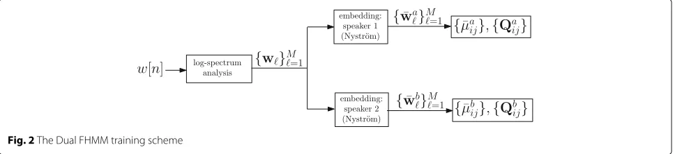
The training procedure of FHMMaand FHMMbis
sum-marized in Algorithm 2. The overall scheme is depicted in Fig. 2.
Algorithm 2Dual FHMM training
1: Compute the log-spectra {u,v}M=1 of the training signalsu[n] andv[n].
2: Compute{λu,u¯}M=1and{λv,v¯}M=1, the embedding of{u}M=1and{v}M=1, respectively.
3: Estimate the HMM models ofSaandSbas in Fig. 1. 4: Define the synthetic mixturew[n]=u[n]+v[n], and
compute its log-spectrum{w}M=1.
5: Embed{w}M=1onto the diffusion space of Sausing the Nyström Extension and obtain w¯aM=1.
6: Embed{w}M=1 onto the diffusion space ofSbusing the Nyström Extension and obtainw¯bM
=1.
7: Compute
¯
μa
ij,μ¯bij,Q¯aij,Q¯bij
S
i,j=1, the Gaussian param-eters of the observation p.d.f.s using (16)–(18).
4.2.2 Latent state estimation
In the test phase a mixed utterance z[n]= a[n]+b[n] is measured, where a[n] and b[n] are the (unknown) separate speech signals. The latent states correspond-ing to z[n] are estimated by embedding z on the two diffusion spaces, yielding{¯za}N=1and{¯zb}N=1, and apply-ing the embedded domain FHMMs, namely FHMMa
and FHMMb, to {¯za}N=1 and{¯zb}N=1, respectively. Each
FHMM is used to infer the latent state of the speaker used for its own embedding. Hence, we use FHMMaonly
to recover the state sequence ofSa, while discarding the
states sequence obtained forSb. The states sequences are
recovered using the factorial Viterbi algorithm with the parameters of FHMMa. It is identical to Algorithm 1, with ¯
za substitutingz. Similarly, FHMMbis used to estimate
the latent states of Sb, i.e., using Algorithm 1 with z¯b instead ofz.
The gist of this approach, as can be deduced from Section 3.3, is that an embedding space, either FHMMaor
FHMMb, encodes the speech attributes of the respective speaker, and hence would best estimate the latent states of the corresponding speaker.
The procedure for estimating the latent state sequence is summarized in Fig. 3.
4.3 Masking
Masking is a common approach in speech separation given latent states, that is often implemented in the STFT domain, which provides a sparse representations of speech signals. The separated log-spectral vectors of the test signal are reconstructed by associating each fre-quency bin of the input signalz, with either Sa or Sb.
There are various ways to define the mask, and here we stick to [36]. Formally, given the estimates of latent states sa = si,aandsb = sj,b, Roweis proposed [36] to estimate the log-spectral domain vector ofSaby
ˆ
ak=
zk μai(k) >μbj(k) m0(k) else
, (19)
wherem0(k)is a tunable parameter that determines the attenuation of the frequency bins. Also recall thatkis the frequency index. In [36], it is proposed to set m0(k) = −∞, ∀k resulting in a hard mask. As the use of a hard mask might result in noticeable distortions and artifacts in the output signals, we applied a soft estimator instead, by settingm0(k)=μai(k)
ˆ
ak=
zk μai(k) >μbi(k)
μa
i(k) else
. (20)
In this estimator, the log-spectral content of the weaker source is not attenuated as in (19), but synthesized accord-ing to the estimated HMM. This maskaccord-ing was shown by Radfar and Dansereau [35] to correspond to the MMSE estimator given a zero model error. Recovering the log-spectrum ofSbis carried out mutatis mutandis.
5 Experimental results
The proposed HFHMM and DFHMM schemes were experimentally verified by studying common state-of-the-art speech separation tasks. The quality of the result is evaluated using both objective criteria and (informal) lis-tening tests. The proposed schemes are compared to the separation scheme proposed by Roweis [36] (for both hard and soft masks), the iterative FHMM-based estimator by Hu and Wang [38], and to the MIXMAX estimator by Radfar and Dansereau [35].
Fig. 3The DFHMM state inference scheme. The states are inferred by applying two FHMMs. Each FHMM infers the states of the speaker whose training set was used to compute its embedding
5.1 Experimental setup
A training set of 450 noiseless sentences per speaker drawn from the speech separation challenge [58] is used. Each sentence is 1–2 s long, and was down-sampled from 25 kHz to 8 kHz to shorten the running time of the code. The STFT was computed using 256 samples long frames, having an overlap of 128 samples between successive frames (50 % overlap). Consequently, each log-spectral STFT feature vector is 129 coefficients long, and a Hann window was used in both the analysis and synthesis stages. On average, the training set of each speaker consisted of 55,000 log-spectral vectors.
The application of the diffusion embedding to the train-ing set is carried out in two steps. First, 30 random sentences per speaker are embedded by extracting the eigenvectors of the Markov matrix defined by the diffu-sion framework. In the second stage, the remainder of the 420 sentences are embedded by applying the Nys-tröm extension. This embedding scheme was chosen due to complexity and memory considerations.
From the complexity aspect, the dimensionality of the Markov matrix determines the number of operations for the DFHMM in the test phase. The embedding of the mixed signal involves the Nyström extension, which is calculated via (11) and thus affected proportionally to the dimensionality of the Markov matrix. It can also be deduced from (12) that the samples creating the Markov matrix, used for calculating the weight functions mea-suring the graph connectivity, should be kept in the memory.
An RBF kernel is used to compute the spectral embed-ding, with kernel bandwidth. In general, a kernel band-width that is too large can result in HMM states which are almost identical, since all the data points are fully con-nected. An excessively small , might result in a model consisting of mostly disconnected graph nodes, with an increased number of states, that might be computation-ally intractable. A kernel bandwidth ∼ 110 was found to be a good compromise, as it retains 5 % of the edges connected. This is a common approach used in previ-ous works on diffusion based embedding [59], where the embedding was shown to be robust to the kernel bandwidth.
Each FHMM uses S = 70 meta-states computed by applying K-means with Euclidean distance measure to the embedded vectors (see Section 3.4). The proposed schemes is evaluated using different combinations of speakers’ gender: male-female, male-male and female-female, where each combination is tested using four pairs of speakers, each pair contributing 15 mixtures. There-fore, each gender combination is evaluated using 60 sen-tences. The pairs of speakers (numbers refer to [58]) are listed in Table 1. The individual signals are noiseless, and the source to interference ratio (SIR) of the mixed sig-nals is set to 0 dB for all experiments (to comply with our model).
When generating the mixed signal w[n] for the DFHMM scheme (refer to (14)), each of the signalsu[n] and v[n] was created by concatenating utterances from the database in a random order. This implementation stems from the unique structure of the utterances. Each sentence is composed of six words that are ordered in the following manner: command, color, preposition, letter, number and an adverb. For example, a valid sentence is “bin blue at Z three please”. Each component of the utter-ances has a final set of possible values. For instance, the command word can be only one of the following: “bin”, “lay”, “place’,’ or “set”. Ifu[n] andv[n] are summed without shuffling the utterances from the database, an undesired situation can occur in which the mixture of the signals depicts only states in which the speakers utter the same word.
Several variants of the proposed schemes were imple-mented to assess the influence of the various components on the performance. First, an ideal DFHMM (iDFHMM)
Table 1Tested speakers. The pairs of speakers used for testing each algorithm, each pair contributing 15 sentences
Male+male Male+female Female+female
1+32 14+25 15+20
14+30 19+20 18+29
19+28 26+34 22+33
26+27 32+23 16+31
with the accurate factorial states, instead of their estimated counterparts, is implemented by computing the embeddings and the meta-states of the separate (unmixed) speakers.
Second, the hard mask (19) and the soft mask (20) are compared, and the corresponding schemes are denoted as DFHMM-H (hard mask), DFHMM-S (soft mask), iDFHMM-H (idealized DFHMM with hard mask) etc.
Third, two training schemes are compared. The first, uses the entire training set to form the Markov matrix P, while in the second, the matrix is based on 30 sen-tences only and the Nyström extension is used to embed the remaining sentences. These variants are denoted as HFHMM-H-E, HFHMM-S-E for the exact embedding, and HFHMM-H-N, HFHMM-S-N for the procedure that utilizes the Nyström extension. Only the Nyström exten-sion based training is used in the DFHMM scheme, as detailed earlier.
The proposed approaches are compared with contem-porary state-of-the-art schemes: (1) the work of Roweis, using 70 HMM states per speaker, that are inferred by the EM procedure. The HMMs are used to define an FHMM, as detailed in [36]; (2) the iterative algorithm by Hu and Wang [38], with the separation part implemented by infer-ring FHMM states for the mixed signal and then applying MAP estimation. As recommended in [38], the FHMM comprises 256 Gaussians per speaker, and a maximum number of 4 iterations is allowed. To reduce the computa-tional complexity, the beam search uses the 16 most likely preceding state pairs.
The MIXMAX estimator by Radfar and Dansereau [35] uses 512 mixtures per GMM, that are trained on the same 450 sentences as the HFHMM and DFHMM schemes. Such a high dimensional GMM per speaker imposes a heavy computational burden. Therefore, we separated the mixed signals only the most probable states pair [35] and, as indicated by the authors, this procedure achieves com-parable scores to that of full estimation. Finally, in order to reduce some of the artifacts and distortions of the hard mask, we set m0(k) = −8, ∀k for the algorithm proposed by Roweis [36], and for the HFHMM and the DFHMM schemes (when the hard mask is applied). This value was chosen to reflect the average level of low power time-frequency bins. It achieved the best balance between speech intelligibility and separation performance.
5.2 Figures-of-merit
In order to quantify the performance of the proposed sep-aration schemes, we utilized the SIR, source to distortion ratio (SDR) and source to artifacts ratio (SAR) criteria, proposed by Vincent et al. [60] and implemented as a Mat-lab toolbox [61]. The SIR measures the attenuation of the interference with respect to the desired speech signal, and the SAR evaluates the level of artifacts (e.g. musical noise)
in the processed signal. The SDR is the desired signal level with respect to the total contribution of all the other distortion factors. The SDR and the SAR criteria are infor-mative when a hard mask is applied. The outcome of the algorithm was also assessed byinformallistening tests.
5.3 Results 5.3.1 HFHMM
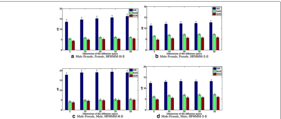
We start by evaluating the performance of the HFHMM scheme. The results are depicted in Fig. 4 for the exact diffusion training. The figure presents the results for the male-female case. It indicates that for the male speaker, 30 dimensions yield the best score, whereas for the female speakerD = 50 is better than D = 30 by 0.7 dB. For the same gender mixture a similar trend is observed, and thus not reported in the figure. The results for the training procedure that incorporates the Nyström extension are less satisfying. Consequently, they are not extensively pre-sented due to space limitations. The quantitative results are reported in Table 2, withD=30 for the male speaker andD=50 for the female speaker across all mixtures. For the male-female mixtures, we report the results related to each gender separately, and for male-male and female-female pairs, we extracted both speakers, and averaged the results. It follows that the HFHMM-S approach outper-forms the HFHMM-H formulation in both the SDR and SAR figures-of-merit for most mixtures, although a degra-dation in the SIR is encountered. The results indicate a performance gap between the H-N, HFHMM-S-N and the HFHMM-H-E, HFHMM-S-E, in favor of the latter. Consequently, we conclude that the Nyström extension leads to performance degradation.
5.3.2 DFHMM
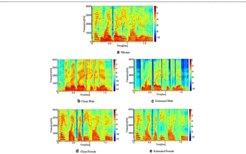
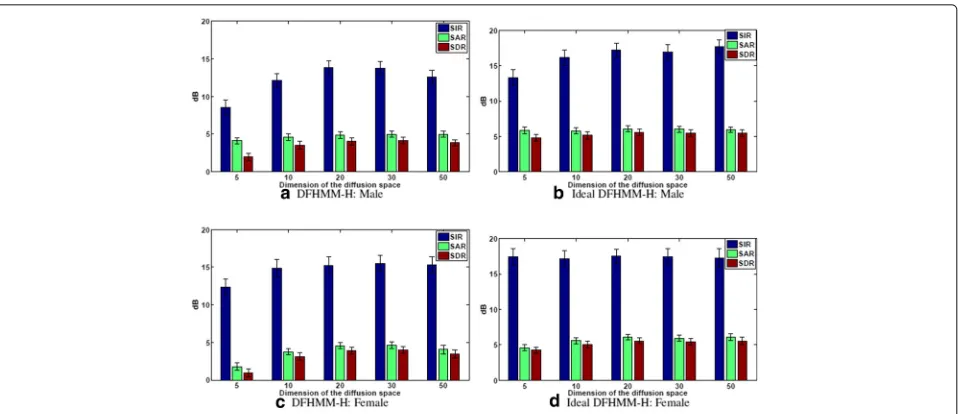
Sonograms and time-frequency maps of the DFHMM-H and DFHMM-S schemes for the male-female mixture are depicted in Figs. 5 and 6. In Fig. 6, the white regions corre-spond to time-frequency bins associated with the female speaker, while the darker ones with the male speaker. It follows that the mask resembles the clustering of the mixed signal (but not perfectly so). Figure 7 depicts the performance metrics of the DFHMM-H estimator and its ideal counterpart iDFHMM-H as a function of the dimen-sionality for the male-female mixture. It follows that an embedding space ofD= 20 suffices for all schemes and the iDFHMM-H outperforms the DFHMM-H by close to 20 % for the male speaker, and∼ 10 % for the female speaker.
Fig. 4HFHMM, separation results for the male-female mixture. Speech separation results measured by SDR, SIR and SAR of the HFHMM scheme for the male-female mixtures. Confidence intervals are also indicated. Training stage was based on exact diffusion maps, without utilizing the Nyström extension
residual interference, being a consequence of the softer mask.
We also subjectively compared the DFHMM-H and the DFHMM-S. The male speaker was recovered by the DFHMM-H without noticeable artifacts. However, the separated female speech sometimes sounds disrupted when a hard mask is used, and applying a soft mask resolved this artifact. Similar trends were observed for the male-male combination.
Application of the DFHMM-H resulted in audible artifacts, that are evident by the low SAR and SDR levels. As in the male-female mixture, applying the DFHMM-S, improves the results, and the ideal estimators,
iDFHMM-H and iDFHMM-S, respectively, outperform their non-ideal counterparts. We attribute this to the pos-sible overlap of the meta-state of speakers of the same gen-der. The female-female mixtures, exhibit similar results to the male-male case.
We further study the effect of the overlapping spectral components, by depicting the hard mask of the female-female mixtures, obtained by the DFHMM-H scheme, in Fig. 8. The white regions of the mask correspond to the time-frequency bins, whereSbis estimated to have higher
spectral content. As most of the mask is white, this indi-cates that Sb is the dominant speaker in the segment.
We fail to identify Sa accurately due to the overlapping
Table 2Quantitative results
Male+female Male+male Female+female Average
Male Female - -
-SIR SAR SDR SIR SAR SDR SIR SAR SDR SIR SAR SDR SIR SAR SDR
Hu and Wang [38] 16.2 7.3 6.5 15.3 8.0 7.0 12.6 6.0 4.6 11.6 5.5 4.0 14.0 6.7 5.5
Roweis-H 18.8 5.4 5.0 15.8 6.1 5.3 10.8 3.3 1.8 9.3 2.6 0.9 13.7 4.3 3.2
Roweis-S 13.0 7.2 5.8 12.6 7.2 5.7 7.7 5.5 2.6 6.5 4.8 1.7 9.9 6.2 3.9
HFHMM-H-E 19.4 5.4 5.1 16.0 6.2 5.4 11.1 3.3 1.8 9.9 3.0 1.3 14.1 4.5 3.4
HFHMM-S-E 13.2 7.2 5.9 12.5 7.2 5.7 7.7 5.5 2.6 6.9 5.2 2.1 10.1 6.3 4.1
HFHMM-H-N 16.9 4.7 4.1 14.4 5.3 4.4 10.6 3.1 1.6 6.4 1.9 -0.8 12.1 3.7 2.3
HFHMM-S-N 12.1 6.4 5.0 11.7 6.3 4.8 7.5 5.2 2.4 4.5 4.0 0.0 8.9 5.5 3.0
DFHMM-H 13.7 5.0 4.1 15.5 4.6 4.0 9.4 2.7 0.7 7.0 4.0 -0.4 11.4 3.9 2.1
DFHMM-S 10.8 6.4 4.7 12.7 5.6 4.5 6.7 4.8 1.5 5.6 4.2 0.4 8.9 5.2 2.3
MIXMAX 15.6 8.6 7.6 15.1 8.6 7.4 10.7 6.8 4.8 9.7 6.3 4.1 12.3 7.6 6.0
Fig. 5DFHMM, illustrative sonograms for the male-female mixture. Male-female mixture. Sonograms of the clean male speech, the clean female speech, the mixture signal and the estimated sources are depicted. The estimated signals were constructed by the DFHMM-S scheme, for a more informative presentation
spectral content of the same gender speakers, especially in the lower frequency band.
5.3.3 Comparison with competing algorithms
In this section, we compare the performance of our proposed algorithms to several single microphone sep-aration algorithms, namely the algorithms proposed by Roweis [36], Hu and Wang [38], specifically the itera-tive FHMM-based inference and MAP estimator variant1, and the MIXMAX-based separation scheme [35]2. For implementing the proposed algorithms we have set the following parameters: for the DFHMM scheme we used
D = 30. For the HFHMM we usedD = 30 for the male speaker and D = 50 for the female speaker. Note that increasingDin the HFHMM only influences its training phase.
The comparative study is summarized in Table 2. For the male speaker in male-female mixture, the HFHMM-H-E outperforms the other estimators with respect to the SIR measure. However, it obtains lower SAR and SDR than the MIXMAX algorithm. Hu and Wang, Roweis-S and HFHMM-S-E also obtain good SAR score, but worse than the MIXMAX. The HFHMM-H-E has a better SIR result also for the female speaker, with the DFHMM-H,
Fig. 7DFHMM, results for the male-female scenario.a,cMale-female separation using the DFHMM-H.b,dusing iDFHMM-H, respectively
Roweis-H scoring below. The SAR and SDR of the MIX-MAX are again superior to the respective measures obtained by the competing algorithms. The algorithm of Hu and Wang also exhibits satisfactory SAR and SDR, although still being inferior to the score obtained by the MIXMAX.
For the male-male mixture, the best SIR result is obtained by Hu and Wang algorithm. The second best results are obtained by the HFHMM-H-E, and then by Roweis-H, HFHMM-H-N and the MIXMAX, respec-tively, with similar performance. The MIXMAX scores the best results in the SAR and SDR measures. The algo-rithm of Hu and Wang demonstrates better measures
for the female-female mixtures in terms of SIR, as well. Again, also for these mixtures the MIXMAX gains the highest SAR score, and shares the best SDR score with Hu and Wang algorithm. However, the HFHMM-S-E and Roweis-S also obtain good SAR results.
By looking at the overall performance, described in the three right-hand-side columns of Table 2, it fol-lows that the HFHMM-H-E and Hu and Wang iterative algorithm obtained the best SIR. The HFHMM-S-E and Hu and Wang also demonstrate reasonable SAR. How-ever, the best SAR and SDR performance was achieved by the MIXMAX algorithm. It is also indicated that using the Nyström extension leads to a degraded performance,
which might explain the relatively disappointing scores of the DFHMM schemes.
Informal listening tests of all estimators and scenarios, demonstrate that there is a large room for improvement. While we notice a slight advantage to the MIXMAX and Hu and Wang algorithms over the proposed algorithms, we claim that the performance differences are rather marginal. Several examples can be found in our website3.
Analyzing both objective results and the informal lis-tening test, we can also observe that better results are obtained for the female-male mixtures, as compared with the female-female and male-male mixtures. This may be attributed to the higher spectral content overlap of the latter two.
We attribute the superior performance of MIXMAX algorithm with respect to the SAR and SDR metrics to the different separation scheme it utilizes. The proposed DFHMM and HFHMM schemes, as well as [36], estimate asingledominant latent state per time-frame, to yield the separation mask, making it susceptible to state estima-tion errors. In contrast, the MIXMAX estimator utilizes a weighted sum of state estimates
ˆ
a= ij
psa=si,a,sb =sj,b|z
ˆ
aij (21)
where aˆij is the estimation of aˆ given z and
sa =si,a,sb =sj,b
. The iterative algorithm of Hu and Wang also utilizes a more sophisticated soft masking procedure (with respect to the procedure discussed in Section 4.3) and hence yields good SAR and SDR. The iterative adaptation of the pre-trained HMMs of the speakers might explain the good SIR performance of Hu and Wang algorithm.
6 Computational complexity of the DFHMM One of the main attributes of the DFHMM algorithm is its computational efficiency (with respect to [36, 38]) due to the use of the low-dimensional embedding. The HFHMM has identical complexity as in [36], since they differ only in the training stage.
The application of the DFHMM algorithm consists of the following steps: spectral analysis and logarithm cal-culation, Nyström extension, factorial Viterbi algorithm, filtering (masking), and spectral synthesis. The procedure in [36] is similar, with the Nyström extension omitted. Another difference is the dimensionality of the factorial Viterbi algorithm. In the DFHMM, it is applied in the (low-dimensional) embedded domain of the mixed signal, whereas in [36] in the (high-dimensional) log-spectrum domain.
It therefore suffices to analyze the computational requirements of the Nyström extension for the DFHMM, and the factorial Viterbi algorithm in order to compare
the computational requirements of both techniques. The number of HMM states for each speaker isS. The analysis refers to a single log-spectral vector of the mixed signal.
6.1 Nyström extension
The Nyström Extension is used to embed a log-spectral vector of the mixed signal using (5), (11), and (12)
λlψl(x˜)= L
i=1
p(x,˜ xi)ψl(xi). (22)
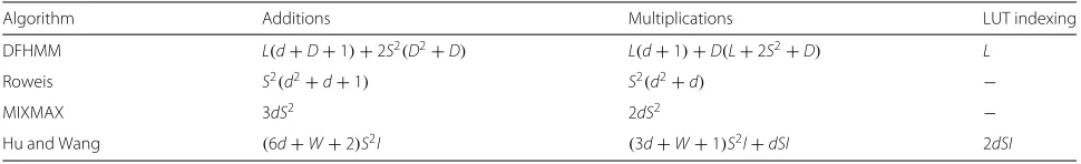
It follows that the number of operations depends on the number of samples in = {xi}Li=1, namelyLDadditions and multiplications.
The computation of the embedding for each point in the datasetxi ∈involves the computation of the kernel
(5), requiringdmultiplications and additions. The expo-nent can be computed using a lookup table (LUT). Hence, (5) is implemented byLd multiplications and additions, andLLUT indexing operations. Finally, note that in (12), the denominator is the same for everyxi ∈ .
Conse-quently, only additional L multiplications and additions are required.
The total number of operations of the Nyström exten-sion is thereforeL(d+D+1)multiplications and additions, andLLUT indexing operations.
6.2 Factorial Viterbi algorithm
The factorial Viterbi is utilized by both the DFHMM and [36], and applied to data of different dimensionality. We start by analyzing the number of operations required by Roweis’s approach [36], as summarized in Algorithm 1. At the preprocessing phase, all expressions are evaluated in advance, except for the p.d.f.p(z|sa = i,sb =j). Writing this p.d.f. explicitly, we have
pz|sa=i,sb =j (23)
= 1
(2π)D|Q|exp
−1
2h
T ijQhij
where|Q|is the determinant of the covariance matrix, and hij=z−μij.
This analysis relates to each time instant. The normal-ization of the Gaussian can be discarded, as it does not affect the maximization. The computational complexity can be further reduced by maximizing the logarithm of the p.d.f. . Hence, onlyhTijQhij,i,j = 1, 2,. . .,S should